Canonical Variate Dissimilarity Analysis for
Process Incipient Fault Detection
Karl Ezra S. Pilario and Yi Cao,
Senior Member, IEEE
Abstract
Early detection of incipient faults in industrial processes is increasingly becoming important, as these faults can slowly develop into serious abnormal events, an emergency situation, or even failure of critical equipment. Multivariate statistical process monitoring methods are currently established for abrupt fault detection. Among these, canonical variate analysis (CVA) was proven to be effective for dynamic process monitoring. However, the traditional CVA indices may not be sensitive enough for incipient faults. In this work, an extension of CVA, called the canonical variate dissimilarity analysis (CVDA), is proposed for process incipient fault detection in nonlinear dynamic processes under varying operating conditions. To handle non-Gaussian distributed data, kernel density estimation was used for computing detection limits. A CVA dissimilarity-based index has been demonstrated to outperform traditional CVA indices and other dissimilarity-based indices, namely DISSIM, RDTCSA, and GCCA, in terms of sensitivity when tested on slowly developing multiplicative and additive faults in a CSTR under closed-loop control and varying operating conditions.
Index Terms
Canonical variate analysis, kernel density estimation, dissimilarity analysis, nonlinear dynamic process.
Manuscript received October 03, 2017; revised December 13, 2017 and February 01, 2018; accepted February 24, 2018. Manuscript received in final form Month xx, 2018. The work of K.E.S. Pilario is supported by the DOST-ERDT Faculty Development Fund of the Republic of the Philippines while at Cranfield University, U.K., Paper no. TII-17-2341 (Corresponding author: K.E.S. Pilario).
The authors are with the School of Water, Energy, and Environment, Cranfield University, MK43 0AL, U.K. (email: [email protected]; [email protected]).
Color versions of one or more of the figures in this paper are available online at http://ieeexplore.ieee.org. Digital Object Identifier:
IEEE Transactions on Industrial Informatics, Volume 14, 2018, Issue 12, pp. 5308-5315 DOI:10.1109/TII.2018.2810822
©2018 IEEE. Personal use of this material is permitted. However, permission to reprint/republish this material for advertising or promotional purposes or for creating new collective works for resale or redistribution to servers or lists, or to reuse any copyrighted component of this work in other works must be obtained from the IEEE.
LIST OFABBREVIATIONS
CSTR Continuous Stirred-tank Reactor
CV Canonical Variable
CVA Canonical Variate Analysis
CVDA Canonical Variate Dissimilarity
Analysis
DD Detection Delay
DIS-SIM Dissimilarity Analysis
FAR False Alarm Rate
GCCA Generalized Canonical Correlation
Analysis
KDE Kernel Density Estimation
MDR Missed Detection Rate
MSPM Multivariate Statistical Process
Monitoring
PCA Principal Components Analysis
PLS Partial Least Squares
RDTCSA
Recursive Dynamic Transformed Component Statistical Analysis
SV Singular Value
SVD Singular Value Decomposition
UCL Upper Control Limit
I. INTRODUCTION
I
NDUSTRIAL process monitoring deals with the detection, identification, diagnosis, and prognosis ofabnormal events, or so-called faults, in industrial processes [1], [2]. A fault is formally defined as
an “unpermitted deviation of at least one parameter of a process from acceptable conditions” [3]. More specifically, process monitoring methods aim to systematically [4]: (1) determine whether a fault has occurred (detection); (2) identify the process variables affected by the fault (identification); (3) determine the type, location, and magnitude of fault (diagnosis); and, (4) predict the evolution of a detected fault
and its effects (prognosis). It is clear that these procedures are important for the safe, reliable, and environmentally benign operation of plants in any industry. Thus, automated industrial process monitoring has been an active field of study for decades now [1].
Widely used data-based fault detection methods, namely Multivariate Statistical Process Monitoring (MSPM) techniques, distinguish faulty from normal process states by establishing statistical thresholds around feature variables extracted from the process historical data [4]. Currently, MSPM techniques are
being developed for nonlinear dynamic processes with the goals of increased sensitivity, early detection,
and minimal false alarms during normal operation. Notable approaches are those based on principal com-ponents analysis (PCA) [5]–[8], partial least squares (PLS) [9], [10], independent component analysis [11], [12], and canonical variate analysis (CVA) [13], [14]. When compared to each other using benchmark case studies such as the Tennessee Eastman plant [4], [13], [15] and a multiphase flow facility [16], CVA-based methods were shown to be advantageous for nonlinear dynamic process monitoring in terms of detection rates and false alarm rates.
However, most existing literature focused on detecting abrupt faults. Isermann [3] distinguished between three types of fault according to how it progresses in time: abrupt, intermittent, and incipient. Abrupt faults are stepwise changes; intermittent faults are random occasional changes; while incipient faults are slowly developing changes. Early detection of incipient faults is more important than detection of abrupt faults for a number of reasons. When left unmanaged, incipient faults increase in severity, leading to more serious abnormal conditions. Even worse, it can lead to equipment failure or an emergency situation [17]. Thus, early detection is valuable for preventive maintenance of equipment and safer operations. Moreover, incipient faults require prognosis [18]. If a fault is detected in its incipient stage, operators may still decide
to continue production; then,predictivemonitoring can aid in subsequent production planning and provide
lead time information before failure of critical assets occur [17], [19].
Unfortunately, incipient faults are more difficult to detect than abrupt faults. At the onset, they may be small enough to be accommodated by robust process control [20] or masked by noise, disturbances, or other faults. Thus, the aforementioned MSPM tools and their detection indices may not be sensitive enough to detect incipient faults.
To address this issue, Harmouche et al. [21] proposed PCA with kernel density estimation (KDE) and
observed subtle differences in the estimated probability distribution of the principal components using the Kullback-Leibler divergence. The method was able to estimate the fault magnitude even when it is
buried in noise. In a similar work, Harrou et al. [22] used the Hellinger distance metric on the nonlinear
PLS algorithm as a measure of dissimilarity between the probability distribution of the latent variables.
al. [15], [23] proposed dissimilarity analysis on data sets (DISSIM), which also observed subtle changes in the data distribution structure. In DISSIM, the differences between a set of eigenvalues of two data sets are
the features being monitored. In a recent study, Zhao et al.[24] extended the DISSIM algorithm for online
incipient fault diagnosis. A recent MSPM technique called Recursive Dynamic Transformed Component Statistical Analysis was also proposed by Shang and Chen [25]. Here, orthogonal transformed components from a sliding window of measurements are obtained recursively. Similar to DISSIM, small changes in the higher-order statistics of the projected data are quantified to form a sensitive index, which was shown to be more reliable than DISSIM and dynamic PCA. However, these dissimilarity-based techniques require a large window width of samples for computing statistical patterns in the data. Also, they do not consider system dynamics, which is essential for monitoring under varying operating conditions.
On a different perspective, Ge et al. [26] used wavelet analysis combined with residual evaluation
to extract an incipient fault feature, and used an improved KDE to form the thresholds. This method, however, requires additional steps to select wavelet basis functions and to tune various parameters so as to achieve acceptable false alarm and missed detection rates. Motivated by the fact that smoothing models such as the moving average and exponentially weighted moving average can detect small shifts in data, Ji et al. [27] proposed to combine them with the conventional MSPM tools, and devised novel generic fault detection indices. Here, “generic” means that the new indices can be applied to any MSPM model of quadratic form. Results have shown increased sensitivity, but only at certain smoothing parameters and weighting factors. Still, none of the above accounted for system dynamics.
To address the difficulty of detecting incipient faults for the case of nonlinear dynamic processes under varying operating conditions, this paper proposes Canonical Variate Dissimilarity Analysis (CVDA). Here, traditional CVA [13], [18] is extended to form a new index based on the dissimilarity between the past-projected and future-past-projected canonical variables, called the canonical variate dissimilarity (CVD) index. CVDA retains the ability of CVA to handle the dynamic issue, as well as non-Gaussianity in the data by using KDE to compute detection limits. Using a closed-loop nonlinear process case study, namely a continuous stirred-tank reactor (CSTR), the CVD index was shown to be superior to the traditional CVA
T2 and Q indices and also to other recent dissimilarity-based indices, in terms of detection time and
reliability. This remains true for both multiplicative and additive incipient fault scenarios considered in this work.
In the next section, the procedure for traditional CVA monitoring is revisited. Section III discusses the motivation behind CVDA and the methodology. Section IV contains the case study description, results, and discussion. The paper is concluded in Section V, along with intended future work.
II. CANONICALVARIATEANALYSIS REVISITED
CVA is a linear dimensionality reduction technique that finds the maximum correlation between any two data sets [4]. Applications of CVA to industrial processes was pioneered by Larimore [28], [29]. As an MSPM tool, the data sets that CVA aims to correlate maximally are the past and future data during normal operation. Details about this method are as follows.
A. CVA Training
Negiz and Cinar [30] established that because industrial processes consist of a large number of process variables operating at controlled conditions, it is useful to assume that the process being monitored has a state-space realization, which is equivalent to representing the system in a vector autoregressive moving-average time-series model with exogenous inputs. In linear state-space form, this model can be written as
x(t+ 1) =Ax(t) +Bu(t) +Kν(t) (1)
y(t) = Cx(t) +Du(t) +ν(t) (2)
where A,B,C,D and K are coefficient matrices, x(t) is the state vector, y(t) is the output observation vector, u(t) is the input vector, and ν(t) are independent noises.
Let uk ∈ <mu andyk∈ <my respectively denote the input and output column vectors from the process
at a certain time point k. For each k, the past data vectors pk and future data vectors fk are collected as
pk= [uTk−1 uTk−2 . . . uTk−p yT k−1 yTk−2 . . . yTk−p] T ∈ <mp (3) fk = h yT k yTk+1 yTk+2 . . . yTk+f−1 iT ∈ <myf (4)
where m =mu+my, and p and f are the number of lags considered in the past and future windows of
data, respectively. The amount of lag is chosen large enough to capture data autocorrelation. The input
vectors, u, are excluded from the future data vectors considering their statistical independence from the
past. Both data vectors are then normalized to zero mean and unit variance.
For a training set with N number of observations, pk and fk for all k ∈ [p+ 1, p+M] are appended
column-wise to form the past and future Hankel matrices
Yp = h pp+1 pp+2 . . . pp+M i ∈ <mp×M (5) Yf = h fp+1 fp+2 . . . fp+M i ∈ <myf×M (6) where M =N −p−f+ 1.
The sample covariance and cross-covariance of the past and future observations can be estimated as Σpp= 1 M −1YpY T p ∈ < mp×mp (7) Σf f = 1 M −1YfY T f ∈ < myf×myf (8) Σf p = 1 M −1YfY T p ∈ < myf×mp. (9)
For training, CVA aims to find linear combinations of Yp and Yf with the maximum correlation. This
can be achieved by a singular value decomposition (SVD) on the scaled Hankel matrix, H:
H=Σ−f f1/2Σf pΣ−pp1/2 =UΣV T
(10)
where U and V contains the left and right singular column vectors of H, and Σ is a diagonal matrix
of ordered singular values (SVs), i.e. Σ = diag(σ1, σ2, . . . , σr,0, . . . ,0) where r is the rank of H and 1≥σ1 ≥σ2 ≥. . .≥σr.
Projection matrices, J =VTΣ−1/2
pp andL=UTΣf f−1/2, are now used to transform Yp andYf to reveal
maximally correlated canonical variables, Cp andCf, projected from the past and future data, respectively:
Cp =JYp ∈ <mp×M (11)
Cf =LYf ∈ <myf×M. (12)
These canonical variables (CVs) are the features used to distinguish normal from faulty process states.
At normal operation, the distributions of Cp and Cf are preserved.
B. CVA Monitoring
Important properties of the SVD in (10) are written below, showing the cross-covariance and covariance of the CVs:
CfCpT =LΣf pJT =Σ·(M −1) (13)
CpCpT =JΣppJT =I·(M −1) (14)
CfCfT =LΣf fLT =I·(M −1). (15) Equation (13) indicates that the SVs, σi(i = 1,2, . . . , r), are the canonical correlations of the CVs.
Based on the SV trend, there exists only n (< r) strongly correlated CVs which explain most of the
system dynamic behavior. Hence, the CV space can be partitioned into two orthogonal subspaces. The
first n CVs span the state subspace, Z, of the system in (1). In other words, the first n CVs at time t,
system residual subspace, E. In traditional CVA-based strategies [4], [13], only the past data vectors are used to reveal the state and residual subspaces:
zk =Jnpk∈ <n (16) ek=Fpk∈ <mp (17) where Jn=VnTΣ −1/2 pp , F= (I−VnVTn)Σ −1/2
pp , zk is the state vector at time k, ek is the model residual
vector at time k, and Vn is a reduced matrix consisting of the first n columns of V. Matrices Jn and F
represent the projection matrices applied to the past data vectors.
Hotelling’s T2 and the Q statistics, two widely used indices in process monitoring, are computed at
each time point k:
Tk2 =zTkzk (18)
Qk =eTkek. (19)
Upper control limits (UCLs) for these two indices can be obtained analytically by assuming that the underlying process data follows a Gaussian distribution. However, this is no longer valid for nonlinear processes under varying operating conditions. To address this, kernel density estimation (KDE) is used
to estimate the probability distributions of T2 and Q [13]. The chosen kernel in this paper is the radial
basis function: K(g) = √1 2πexp −g 2 2 . (20)
The UCLs serve as thresholds between normal and abnormal conditions. Given a significance level,
α, the UCLs denoted by T2
UCL and QUCL can be obtained such that P(T2 < TUCL2 ) = α and P(Q <
QUCL) =α, with P(x < b) = Z b −∞ 1 M h M X k=1 K x−xk h dx (21)
where xk, k = 1,2,· · · , M are the samples of x and h is the kernel bandwidth. More details for KDE
are given in [13].
Finally, for online monitoring, the state and residuals are continuously calculated from real-time data
using (16) and (17). The T2 and Qat every sampling point are then obtained using (18) and (19). A fault
is detected when any one of these indices exceed its corresponding UCL, T2
III. CANONICALVARIATEDISSIMILARITY ANALYSIS
Process incipient faults manifest as small shifts in the data caused by decay in process parameters, unwanted material build-up, or sensor drifts, etc. Motivated by the ability of CVA to find maximum correlations between past and future data, one can detect small data shifts by checking how well future CVs are predictable from past CVs, based on the state-space model trained during normal conditions. This leads to the notion of assessing the dissimilarity between the past- and future-projected CVs for indicating process health.
A statistical index that quantifies model residuals in the CVA state-subspace has been suggested by
Larimore [29]. In that work, the residuals, , are generated as
k =Lnfk−ΣnJnpk ∈ <n (22)
where subscript k denotes the kth sample, subscript n denotes the number of states in the CVA model
(which reduces J and L to the first n rows), and Σn = diag(σ1, σ2, . . . , σn). To our knowledge, the T2 index formed from the residuals in (22) is underexplored among numerous CVA-based fault detection
methods. In one study, Juricek et al. [31] found that an index similar to (22) outperforms a Kalman filter
residuals-based index with respect to sensitivity, although their index requires state-space matrices to be calculated, hence is not data-driven. Analogous formulations of (22) are also found in recent works by
Jiang et al. [32] and Chen et al. [33] except that canonical correlation analysis was applied between
process inputs and outputs instead of past and future data. For our work, the residuals in (22) are taken as dissimilarity features which can have a new meaning for detecting incipient faults. These features are measures of the departure of the current actual states (estimated from the future vector that includes current measurements) from the states predicted by the CVA model using past data.
To derive an index from (22), let d denote the dissimilarity features, i.e.d :=. Also, letZf =LnYf
and Zp =JnYp denote the future- and past-projected states, respectively. Since ZfZTf =ZpZTp = I and
ZfZTp =Σn, the covariance of d can be estimated as
Σdd = 1
M −1(Zf −ΣnZp)(Zf −ΣnZp)
T (23)
=I−Σ2n∈ <n×n. (24)
At normal operation, the dissimilarity features are distributed around a zero mean. Thus, a detection index can be formed as the squared Mahalanobis distance of the dissimilarity features from zero, i.e.
by taking the sum of squares of the dissimilarities dk ∈ <n, for each time point k, normalized by the
covariance matrix, Σdd: Dk=dTk(I−Σ 2 n) −1d k. (25)
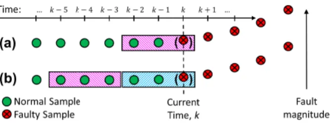
Fig. 1. Initial stage of a fault and how it is captured by (a) traditional CVA indices; and (b) CVD index. Legend: past vector - pink; future vector - blue.
Hereafter, D is referred to as the canonical variate dissimilarity (CVD) index. Unlike the CVA T2 and
Q indices in (18)-(19) which only take information from the past data, the CVD index takes information
from both past and future data. For online monitoring using CVA, each new sample enters only the past
data vector of length p. On the other hand, for CVD, each new sample enters the future data vector, while
the past data vector is formed from p samples,f lags earlier. Thus, in the early stage of an incipient fault
shown in Fig. 1 (where p =f = 3), small shifts can be better captured as discrepancies found between
the past and future data.
In this paper, KDE is adopted to estimate the distribution of D, and subsequently solve for the upper
control limit of D, denoted byDUCL. All three indicesT2,Q, andD, will be used for monitoring incipient
faults in nonlinear dynamic processes under the framework referred to as canonical variate dissimilarity
analysis (CVDA). A sample is considered faulty if eitherT2, Q, orD, exceeds their respective thresholds,
TUCL2 , QUCL, and DUCL, for that sample.
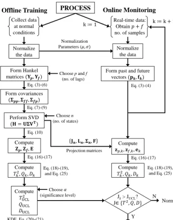
In summary, the CVDA procedure for incipient fault detection is given in Fig. 2. The goal of offline training is to generate the UCLs and the projection matrices. On the other hand, online monitoring consists
of the continuous collection of a moving window of samples of length p+f (Fig. 1b), which are used
to check if the process is normal or faulty.
IV. CASE STUDY
In this section, the proposed CVDA is evaluated using a closed-loop continuous stirred-tank reactor (CSTR) case study, designed especially for simulating incipient faults.
A. Process Description
A number of works, such as [6], [8], [10], [17], [18], [31], used different versions of a CSTR for evaluating process monitoring methods. A general first-principles model of a constant-holdup, jacketed
PROCESS Collect data at normal conditions Real-time data: Obtain 𝑝 + 𝑓 no. of samples Online Monitoring Normalize the data Normalize the data Normalization Parameters (𝜇, 𝜎) Form Hankel matrices (𝐘𝒑, 𝐘𝒇) Eq. (3)-(6) Offline Training
Form past and future vectors (𝐩𝒌, 𝐟𝒌) Eq. (3)-(4) Form covariances (𝚺𝒑𝒑, 𝚺𝒇𝒇, 𝚺𝒇𝒑) Perform SVD (𝐇 = 𝐔𝚺𝐕𝐓) Compute 𝐙𝒑, 𝐙𝒇, 𝐄 Eq. (16)-(17) Compute 𝐳𝑝,𝑘, 𝐳𝑓,𝑘, 𝐞𝑘 Eq. (16)-(17) Eq. (7)-(9) Eq. (10) Choose pand f (no. of lags) Choose n (no. of states) 𝐉𝒏, 𝐋𝒏, 𝚺𝒏, 𝐅 Compute 𝑇𝑘2, 𝑄𝑘, 𝐷𝑘 Compute 𝑇𝑘2, 𝑄𝑘, 𝐷𝑘 Compute 𝑇UCL2 𝑄UCL 𝐷UCL KDE, Eq. (20)-(21) Jk> JUCL? J∈ {𝑇2, 𝑄, 𝐷} Normal Faulty N Y k ≔ 1 k ≔ k + 1 Eq. (18)-(19), and Eq. (25) Eq. (18)-(19), and Eq. (25) Projection matrices Choose 𝛼 (significance level)
Fig. 2. CVDA procedure for process incipient fault detection.
dC dt = Q V (Ci−C)−akC+ν1 (26) dT dt = Q V (Ti−T)−a (∆Hr)kC ρCp −b U A ρCpV (T −Tc) +ν2 (27) dTc dt = Qc Vc (Tci−Tc) +b U A ρcCpcVc (T −Tc) +ν3 (28)
where the inputs areu=hCi Ti Tci
iT
, the outputs arey=hC T Tc Qc
iT
,νiare process noise, and
k is an Arrhenius-type rate constant,k =k0exp −RTE
.Table I gives the parameter values in Eq. (26)-(28).
The CSTR Simulink model used in this work is available online [34].
The CSTR schematic in Fig. 3 shows the measurement locations and the control strategy: Reactor
temperature,T, is maintained by manipulating the coolant flow rate,Qc. To be more realistic, the controller
(Kc = 1.0 and τI = 0.2) is set to saturate below 10 L/min and above 200 L/min. Saturation is important
for simulating cases where an incipient fault becomes too severe to be accommodated by controls. In the
model, a and b are both equal to 1.00 at normal operation. By decaying their values toward zero, one can
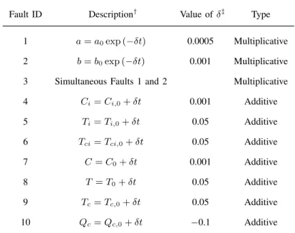
simulate catalyst decay and heat transfer fouling, respectively. Other faults in the system are sensor drifts on each of the 7 measured variables. Details on these incipient fault scenarios are given in Table II.
TABLE I
CONSTANT VALUES IN THECSTRMODEL
Parameter Description Value Units
Q Inlet flow rate 100.0 L/min
V Tank volume 150.0 L
Vc Jacket volume 10.0 L
∆Hr Heat of reaction −2.0×10⁵ cal/mol
U A Heat transfer coefficient 7.0×10⁵
cal/min/K
k0 Pre-exponential factor tok 7.2×10¹⁰ min−1
E/R Activation energy 1.0×10⁴ K
ρ, ρc Fluid density 1000 g/L
Cp, Cpc Fluid heat capacity 1.0 cal/g/K
TABLE II
INCIPIENT FAULT SCENARIOS IN THECSTR
Fault ID Description† Value ofδ‡ Type
1 a=a0exp (−δt) 0.0005 Multiplicative
2 b=b0exp (−δt) 0.001 Multiplicative
3 Simultaneous Faults 1 and 2 Multiplicative 4 Ci=Ci,0+δt 0.001 Additive 5 Ti=Ti,0+δt 0.05 Additive 6 Tci=Tci,0+δt 0.05 Additive 7 C=C0+δt 0.001 Additive 8 T =T0+δt 0.05 Additive 9 Tc=Tc,0+δt 0.05 Additive 10 Qc=Qc,0+δt −0.1 Additive †
Alltin minutes. Subscript 0 refers to nominal value.
‡
Theδ commands the rate of fault progression.
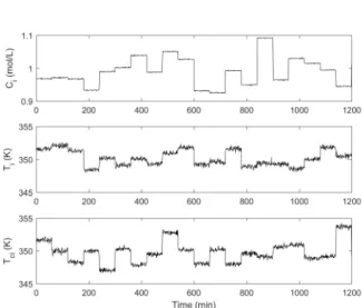
Fault-free and faulty data sets were generated from the CSTR simulation for 20 h of operation, while
varying the operating conditions by perturbing the inputs, u, randomly around their nominal values every
60 min as in Fig. 4. The sampling interval for all variables is 1 min. Note that input disturbances can bring out system dynamics, such that measurements become temporally correlated and non-Gaussian-distributed due to the process nonlinearity. This merits the use of CVA and KDE for the CSTR case study, as these are
Fig. 3. Schematic of the closed-loop CSTR.
Fig. 4. Input variables sample data set from CSTR simulation.
recommended for nonlinear dynamic process monitoring [13]. In faulty data sets, the fault is introduced only after 200 min of normal operation. To evaluate the performance robustly, 250 faulty data sets are generated in each fault scenario, differing in the random seeds for the process noise, measurement noise, and input disturbances. Performance metrics for monitoring (see Section IVc) are averaged across all trials.
B. CVDA Training
A single fault-free data set was used for CVDA training. Firstly, the number of time lags to consider
in the past and future data (p and f) were chosen using autocorrelation analysis [30] on the output
training data, y. For the case study, it was found that five number of lags is the maximum after which
autocorrelations in data become insignificant at 5% confidence bounds. Thus, p and f are both set to 5.
SVD was then performed on the scaled Hankel matrix, which was formed based on p and f. The
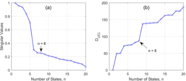
number of states, n, in the CVA model was then estimated from the training data. A plot of the singular
values (SVs) computed from (10) is shown in Fig. 5a, which are the non-zero elements in the diagonal
Fig. 5. Analysis on choosing the number of CVA states, n, using: (a) Singular Value (SV) plot; and (b)DUCL-vs-nplot (99.9% significance level).
commonly called the dominant singular value method of selecting n. Other ways of selecting n include
using the Akaike Information Criterion [4] or minimizing false alarms during cross-validation [16].
In this work, we propose to use DUCL-vs-n plots to augment the dominant singular value method in
selecting n. If we proceed with the CVDA procedure until DUCL is computed, we can produce a plot
of DUCL’s against increasing choices of n (Fig. 5b). Intuitively, DUCL measures how precisely the CVA
model predicts the future state. For small values of n, prediction is precise because the dissimilarities
between the firstn past and future CVs are small, i.e.DUCL is low. For largen, the dissimilarities become
large due to capture of weakly correlated CVs, i.e.DUCLis high. Therefore, a large jump in theDUCL-vs-n
curve indicates a sudden entry of unnecessary noise into the model, i.e. the clear boundary between the
state and residual subspaces. Figure 5b shows the DUCL-vs-n plot for the CSTR training data. The point
right before the jump in the curve is located at n = 8. This choice agrees with the SV plot on Fig. 5a,
where the “knee” appears at n≥6. Thus, for the case study,n is set to 8. From here, the CVA model is
now trained and the actual detection limits are computed using KDE at 99.9% significance level.
C. CVDA Monitoring
In this work, monitoring performance is evaluated according to detection delay (DD), false alarm rate (FAR), missed detection rate (MDR), and visually using monitoring charts (Fig. 6). Note that because we are monitoring slowly developing faults, detection time could be ambiguous, i.e. the index may spend a considerable amount of time fluctuating around the detection limit before it fully registers a fault. Thus,
detection time is defined as the first time after 5 consecutive alarms were raised. Accordingly, DD is the period between the start of the fault and the detection time. FAR and MDR are computed as:
FAR= no. of samples (J > JUCL|fault-free)
total samples (fault-free) ×100% (29)
MDR= no. of samples (J < JUCL|fault)
Fig. 6. Monitoring charts for Fault 3 using: (a,b) GCCA; (c,d) CVA; (e) RDTCSA; (f) CVDA. See Section IVc for implementation details. Legend: Dashdot - upper control limit (UCL); Dash - start of fault; Solid - detection index.
Fig. 7. Output variables sample data set under Fault 3 conditions: catalyst decay and heat transfer fouling were both introduced at 200 min.
where J = {T2, Q, D}. A good detection index must have low DD, low FAR, and low MDR. DD is
particularly important for assessing the sensitivity of a detection index.
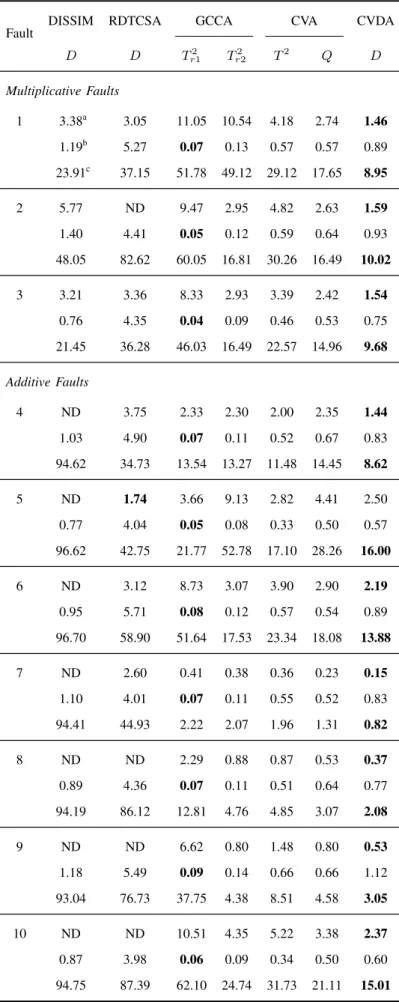
Table III compares the proposed CVD index with the traditional CVA indices [18] and other dissimilarity-based indices from recent works: dynamic DISSIM [23], Recursive Dynamic Transformed Component Statistical Analysis (RDTCSA) [25], and Generalized Canonical Correlation Analysis (GCCA) [33]. For the dynamic DISSIM and RDTCSA indices, five lagged variables (same as CVDA) and a window width of 120 samples were used. For RDTCSA, the sample mean, variance, skewness, and kurtosis are included
in the feature vector, scalarized by the `∞-norm. For GCCA, both Tr21 and Tr22 were used as defined
in [33], except that the UCL was not computed using randomized algorithms. Rather, all UCLs in this study were computed using KDE at 99.9% significance level. Detection delays in Table III are reported
in units of hours due to the slow rate of progression designed for the incipient faults (see Table II). This design also makes the distinction between methods more pronounced.
In terms of DD and MDR, the CVD index is seen to be most sensitive for all fault scenarios. The dynamic DISSIM and RDTCSA incurred non-detection for some faults, as they do not consider the system dynamics that can be inferred from the temporal correlation in the data. Although the RDTCSA index detected Fault 5 the earliest, the high MDR reveals that the index struggles to cross the detection limit.
The GCCA indices, T2
r1 and Tr22, are more reliable, as one of them is sensitive to the faults where the
other is not (e.g. Faults 5 and 6). Consistent with the findings in [33],T2
r2 is often more sensitive than Tr21.
Also, the GCCA indices appear to incur the least false alarms during normal operation. Indeed, although the CVD index is most sensitive, it incurs slightly more false alarms. Nonetheless, the CVD index is most reliable in terms of combined FARs and MDRs. These results validate the importance of using the dissimilarity between past and future states for incipient fault detection, rather than past states only, as in traditional CVA.
To appreciate the performance of the CVD index, sample monitoring charts for Fault 3 are shown in
Fig. 6, with the corresponding y data in Fig. 7. Fault 3 leads to conflicting behavior (at 600 min) in
the affected variables because the rates of catalyst decay and heat transfer fouling were set so as to keep opposing each other [18]. Eventually, failure occurs after 1085 min. Fig. 6f shows how the proposed CVD index achieves the earliest detection time among the indices being compared, at 295 min. This detection time may not be achieved by mere human inspection on Fig. 7. Thus, using this index, more lead time before failure is realized. Furthermore, it is beneficial for an index to properly reflect fault severity even as it progresses above the UCL. This trait is best observed in the CVD index as well.
The charts in Fig. 6 also marked false alarms. It was found that false alarms mostly occur at times when inputs change abruptly (Fig. 4), causing unrecognized transients in the data (Fig. 7). Thus, one way to lessen false alarms is to train a nonlinear model [14] for CVDA that may recognize these transients. This is left for future work.
V. CONCLUSION
In this paper, the importance of incipient fault detection, rather than abrupt fault, in industrial processes is highlighted. For dynamic process monitoring, the traditional CVA detection method is recognized. This work now extends the CVA framework to emphasize that the assessment of dissimilarity between past
and future states gives a more sensitive index than the traditional T2 and Q for incipient fault detection.
A method for subspace partitioning using DUCL-vs-n plots is also proposed. The new framework, called
canonical variate dissimilarity analysis (CVDA), is intended for nonlinear dynamic process monitoring of incipient faults under varying process operating conditions.
Using a CSTR case study designed to simulate ten slowly developing faults, the CVD index was shown
to be superior to the CVA T2 and Q indices, the dynamic DISSIM, RDTCSA, and the GCCA indices
in terms of sensitivity. However, the CVD index incurred more false alarms, mostly occurring when operating conditions change abruptly. This can be lessened by using a nonlinear feature extraction step for CVDA. Other ways to quantify statistical pattern dissimilarity between CVs also require further study. Lastly, diagnosis and prognosis methods from the CVDA framework can be developed for incipient fault monitoring in the future.
REFERENCES
[1] M. Reis and G. Gins, “Industrial Process Monitoring in the Big Data/Industry 4.0 Era: from Detection, to Diagnosis, to Prognosis,”
Processes, vol. 5, no. 3, p. 35, 2017.
[2] Y. Shu, L. Ming, F. Cheng, Z. Zhang, and J. Zhao, “Abnormal situation management: Challenges and opportunities in the big data era,”Computers and Chemical Engineering, vol. 91, pp. 104–113, 2016.
[3] R. Isermann, “Model-based fault-detection and diagnosis - Status and applications,”Annual Reviews in Control, vol. 29, no. 1, pp. 71–85, 2005.
[4] L. H. Chiang, E. L. Russell, and R. D. Braatz,Fault Detection and Diagnosis in Industrial Systems. London: Springer-Verlag, 2005. [5] W. Ku, R. H. Storer, and C. Georgakis, “Disturbance detection and isolation by dynamic principal component analysis,”Chemometrics
and Intelligent Laboratory Systems, vol. 30, no. 1, pp. 179–196, 1995.
[6] S. W. Choi, C. Lee, J. M. Lee, J. H. Park, and I. B. Lee, “Fault detection and identification of nonlinear processes based on kernel PCA,”Chemometrics and Intelligent Laboratory Systems, vol. 75, no. 1, pp. 55–67, 2005.
[7] R. T. Samuel and Y. Cao, “Nonlinear process fault detection and identification using kernel PCA and kernel density estimation,”Systems Science & Control Engineering, vol. 4, no. 1, pp. 165–174, 2016.
[8] M. Mansouri, M. Nounou, H. Nounou, and N. Karim, “Kernel PCA-based GLRT for nonlinear fault detection of chemical processes,”
Journal of Loss Prevention in the Process Industries, vol. 40, pp. 334–347, 2016.
[9] C. Shang, X. Huang, J. A. K. Suykens, and D. Huang, “Enhancing dynamic soft sensors based on DPLS: A temporal smoothness regularization approach,”Journal of Process Control, vol. 28, pp. 17–26, 2015.
[10] C. Botre, M. Mansouri, M. Nounou, H. Nounou, and M. N. Karim, “Kernel PLS-based GLRT method for fault detection of chemical processes,”Journal of Loss Prevention in the Process Industries, vol. 43, pp. 212–224, 2016.
[11] J. Fan and Y. Wang, “Fault detection and diagnosis of non-linear non-Gaussian dynamic processes using kernel dynamic independent component analysis,”Information Sciences, vol. 259, pp. 369–379, 2014.
[12] G. Stefatos and A. B. Hamza, “Dynamic independent component analysis approach for fault detection and diagnosis,”Expert Systems with Applications, vol. 37, no. 12, pp. 8606–8617, 2010.
[13] P.-E. Odiowei and Yi Cao, “Nonlinear Dynamic Process Monitoring Using Canonical Variate Analysis and Kernel Density Estimations,”
IEEE Transactions on Industrial Informatics, vol. 6, no. 1, pp. 36–45, 2010.
[14] R. T. Samuel and Y. Cao, “Kernel canonical variate analysis for nonlinear dynamic process monitoring,”IFAC-PapersOnLine, vol. 28, no. 8, pp. 605–610, 2015.
[15] M. Kano, K. Nagao, S. Hasebe, I. Hashimoto, H. Ohno, R. Strauss, and B. Bakshi, “Comparison of statistical process monitoring methods: application to the Eastman challenge problem,”Computers & Chemical Engineering, vol. 24, no. 2-7, pp. 175–181, 2000. [16] C. Ruiz-C´arcel, Y. Cao, D. Mba, L. Lao, and R. T. Samuel, “Statistical process monitoring of a multiphase flow facility,” Control
Engineering Practice, vol. 42, pp. 74–88, 2015.
[17] B. C. Juricek, D. E. Seborg, and W. E. Larimore, “Predictive monitoring for abnormal situation management,” Journal of Process Control, vol. 11, no. 2, pp. 111–128, 2001.
[18] K. E. Pilario and Y. Cao, “Process incipient fault detection using canonical variate analysis,” in 2017 23rd International Conference on Automation and Computing (ICAC). IEEE, sep 2017, pp. 1–6.
[19] G. Vachtsevanos, F. L. Lewis, M. Roemer, A. Hess, and B. Wu,Intelligent Fault Diagnosis and Prognosis for Engineering Systems. John Wiley & Sons, Inc., 2006.
[20] X. Zhang, M. M. Polycarpou, and T. Parisini, “A robust detection and isolation scheme for abrupt and incipient faults in nonlinear systems,”IEEE Transactions on Automatic Control, vol. 47, no. 4, pp. 576–593, 2002.
[21] J. Harmouche, C. Delpha, and D. Diallo, “Incipient fault detection and diagnosis based on Kullback-Leibler divergence using Principal Component Analysis: Part I,”Signal Processing, vol. 94, no. 1, pp. 278–287, 2014.
[22] F. Harrou, M. Madakyaru, and Y. Sun, “Improved nonlinear fault detection strategy based on the Hellinger distance metric: Plug flow reactor monitoring,”Energy and Buildings, vol. 143, pp. 149–161, 2017.
[23] M. Kano, S. Hasebe, I. Hashimoto, and H. Ohno, “Statistical Process Monitoring Based on Dissimilarity of Process Data,” IFAC Proceedings Volumes, vol. 33, no. 10, pp. 231–236, jun 2002.
[24] C. Zhao and F. Gao, “A sparse dissimilarity analysis algorithm for incipient fault isolation with no priori fault information,”Control Engineering Practice, vol. 65, pp. 70–82, 2017.
[25] J. Shang and M. Chen, “Recursive Dynamic Transformed Component Statistical Analysis for Fault Detection in Dynamic Processes,”
IEEE Transactions on Industrial Electronics, vol. 65, no. 1, pp. 578–588, 2018.
[26] W. Ge, J. Wang, J. Zhou, H. Wu, and Q. Jin, “Incipient fault detection based on fault extraction and residual evaluation,”Industrial and Engineering Chemistry Research, vol. 54, no. 14, pp. 3664–3677, 2015.
[27] H. Ji, X. He, J. Shang, and D. Zhou, “Incipient fault detection with smoothing techniques in statistical process monitoring,”Control Engineering Practice, vol. 62, pp. 11–21, 2017.
[28] W. E. Larimore, “Canonical variate analysis in identification, filtering, and adaptive control,”Proceedings of the IEEE Conference on Decision and Control, vol. 2, pp. 596–604, 1990.
[29] ——, “Optimal Reduced Rank Modeling, Prediction, Monitoring and Control using Canonical Variate Analysis,” IFAC Proceedings Volumes, vol. 30, no. 9, pp. 61–66, 1997.
[30] A. Negiz and A. Cinar, “Statistical Monitoring of Multivariable Dynamic Processes with State-Space Models,”AIChE Journal, vol. 43, no. 8, pp. 2002–2020, 1997.
[31] B. C. Juricek, D. E. Seborg, and W. Larimore, “Fault Detection Using Canonical Variate Analysis,”Industrial & Engineering Chemistry Research, vol. 43, pp. 458–474, 2004.
[32] Q. Jiang, S. X. Ding, Y. Wang, and X. Yan, “Data-Driven Distributed Local Fault Detection for Large-Scale Processes Based on the GA-Regularized Canonical Correlation Analysis,”IEEE Transactions on Industrial Electronics, vol. 64, no. 10, pp. 8148–8157, 2017. [33] Z. Chen, S. X. Ding, T. Peng, C. Yang, and W. Gui, “Fault Detection for Non-Gaussian Processes Using Generalized Canonical Correlation Analysis and Randomized Algorithms,”IEEE Transactions on Industrial Electronics, vol. 65, no. 2, pp. 1559–1567, feb 2018.
[34] “Feedback controlled cstr process for fault simulation,” 2018. [Online]. Available: https://uk.mathworks.com/matlabcentral/fileexchange/66189-feedback-controlled-cstr-process-for-fault-simulation
Karl Ezra S. Pilarioreceived his B.Sc. and M.Sc. degrees in Chemical Engineering from the University of
the Philippines, Diliman, in 2012 and 2015, respectively. He is currently pursuing a Ph.D. degree at Cranfield University, Cranfield, U.K.
He is also an Assistant Professor on study leave from the Department of Chemical Engineering at University of the Philippines, Diliman. His research interests are in Process Monitoring and other data-driven methods in Process Systems Engineering.
Yi Cao(M’96, SM’10) received the M.Sc. degree in Control Engineering from Zhejiang University, China in 1985 and the Ph.D. degree in Engineering from the University of Exeter, United Kingdom in 1996.
He is a Reader with the School of Water, Energy and Environment, Cranfield University. His research interests are in Advanced Process Control, including Plant-wide Control, Nonlinear System Identification, Nonlinear Model Predictive Control and Process Monitoring.
TABLE III
MONITORINGPERFORMANCE†FOR THECSTRINCIPIENT FAULTS
Fault
DISSIM RDTCSA GCCA CVA CVDA
D D Tr21 T 2 r2 T 2 Q D Multiplicative Faults 1 3.38a 3.05 11.05 10.54 4.18 2.74 1.46 1.19b 5.27 0.07 0.13 0.57 0.57 0.89 23.91c 37.15 51.78 49.12 29.12 17.65 8.95 2 5.77 ND 9.47 2.95 4.82 2.63 1.59 1.40 4.41 0.05 0.12 0.59 0.64 0.93 48.05 82.62 60.05 16.81 30.26 16.49 10.02 3 3.21 3.36 8.33 2.93 3.39 2.42 1.54 0.76 4.35 0.04 0.09 0.46 0.53 0.75 21.45 36.28 46.03 16.49 22.57 14.96 9.68 Additive Faults 4 ND 3.75 2.33 2.30 2.00 2.35 1.44 1.03 4.90 0.07 0.11 0.52 0.67 0.83 94.62 34.73 13.54 13.27 11.48 14.45 8.62 5 ND 1.74 3.66 9.13 2.82 4.41 2.50 0.77 4.04 0.05 0.08 0.33 0.50 0.57 96.62 42.75 21.77 52.78 17.10 28.26 16.00 6 ND 3.12 8.73 3.07 3.90 2.90 2.19 0.95 5.71 0.08 0.12 0.57 0.54 0.89 96.70 58.90 51.64 17.53 23.34 18.08 13.88 7 ND 2.60 0.41 0.38 0.36 0.23 0.15 1.10 4.01 0.07 0.11 0.55 0.52 0.83 94.41 44.93 2.22 2.07 1.96 1.31 0.82 8 ND ND 2.29 0.88 0.87 0.53 0.37 0.89 4.36 0.07 0.11 0.51 0.64 0.77 94.19 86.12 12.81 4.76 4.85 3.07 2.08 9 ND ND 6.62 0.80 1.48 0.80 0.53 1.18 5.49 0.09 0.14 0.66 0.66 1.12 93.04 76.73 37.75 4.38 8.51 4.58 3.05 10 ND ND 10.51 4.35 5.22 3.38 2.37 0.87 3.98 0.06 0.09 0.34 0.50 0.60 94.75 87.39 62.10 24.74 31.73 21.11 15.01 †
All results were averaged across 250 faulty data sets monitored in each Fault ID. Boldfaced entries are the best values in each row.
a
First row: Detection delays (DD, hours); ND = “not detected (consis-tently for 5 consecutive sampling times)”.
b
Second row: False alarm rates (FAR, %), Eq. (29).
c