October 2009, Volume 32, Issue 3. http://www.jstatsoft.org/
An Object-Oriented Framework for Robust
Multivariate Analysis
Valentin Todorov
UNIDO
Peter Filzmoser
Vienna University of Technology
Abstract
Taking advantage of the S4 class system of the programming environment R, which facilitates the creation and maintenance of reusable and modular components, an object-oriented framework for robust multivariate analysis was developed. The framework resides in the packagesrobustbaseandrrcovand includes an almost complete set of algorithms for computing robust multivariate location and scatter, various robust methods for principal component analysis as well as robust linear and quadratic discriminant analysis. The design of these methods follows common patterns which we call statistical design patterns in analogy to the design patterns widely used in software engineering. The application of the framework to data analysis as well as possible extensions by the development of new methods is demonstrated on examples which themselves are part of the package rrcov.
Keywords: robustness, multivariate analysis, MCD, R, statistical design patterns.
1. Introduction
Outliers are present in virtually every data set in any application domain, and the identifica-tion of outliers has a hundred years long history. Many researchers in science, industry and economics work with huge amounts of data and this even increases the possibility of anomalous data and makes their (visual) detection more difficult. Taking into account the multivariate aspect of the data, the outlyingness of the observations can be measured by the Mahalanobis distance which is based on location and scatter estimates of the data set. In order to avoid the masking effect, robust estimates of these parameters are called for, even more, they must
possess a positive breakdown point. The estimates of the multivariate location vectorµand
the scatter matrix Σ are also a cornerstone in the analysis of multidimensional data, since
they form the input to many classical multivariate methods. The most common estimators of multivariate location and scatter are the sample meanx¯ and the sample covariance matrix
S, i.e., the corresponding MLE estimates. These estimates are optimal if the data come from a multivariate normal distribution but are extremely sensitive to the presence of even a few outliers (atypical values, anomalous observations, gross errors) in the data. If outliers are present in the input data they will influence the estimatesx¯ and S and subsequently worsen the performance of the classical multivariate procedure based on these estimates. Therefore it is important to consider robust alternatives to these estimators and actually in the last two decades much effort was devoted to the development of affine equivariant estimators possessing a high breakdown point. The most widely used estimators of this type are the
minimum covariance determinant (MCD) estimator ofRousseeuw(1985) for which also a fast
computing algorithm was constructed—Rousseeuw and Van Driessen(1999), the S estimators
(Davies 1987) and the Stahel-Donoho estimator introduced byStahel(1981a,b) and Donoho (1982) and studied byMaronna and Yohai (1995). If we give up the requirement for affine equivariance, estimators like the one ofMaronna and Zamar (2002) are available and the re-ward is an extreme gain in speed. Substituting the classical location and scatter estimates by their robust analogues is the most straightforward method for robustifying many multivariate procedures like principal components, discriminant and cluster analysis, canonical correlation, etc. The reliable identification of multivariate outliers which is an important task in itself, is another approach to robustifying many classical multivariate methods.
Some of these estimates and procedures became available in the popular statistical packages likeS-PLUS,SAS, MATLABas well as in R but nevertheless it is recognized that the robust methods have not yet replaced the ordinary least square techniques as it could be expected (Morgenthaler 2007; Stromberg 2004). One reason is the lack of easily accessible and easy to use software, that is software which presents the robust procedures as extensions to the classical ones—similar input and output, reasonable defaults for most of the estimation options and visualization tools. As far as the easiness of access is concerned, the robust statistical
methods should be implemented in the freely available statistical software package R, (R
Development Core Team 2009), which provides a powerful platform for the development of statistical software. These requirements have been defined in the project “Robust Statistics
andR”, seehttp://www.statistik.tuwien.ac.at/rsr/, and a first step in this direction was
the initial development of the collaborative packagerobustbase (Rousseeuw et al.2009) with the intention that it becomes theessential robust statistics Rpackage covering the methods described in the recent bookMaronna et al.(2006).
During the last decades the object-oriented programming paradigm has revolutionized the style of software system design and development. A further step in the software reuse are the object oriented frameworks (seeGammaet al.1995) which provide technology for reusing both the architecture and the functionality of software components. Taking advantage of the new S4 class system (Chambers 1998) of Rwhich facilitate the creation of reusable and modular components an object-oriented framework for robust multivariate analysis was implemented. The goal of the framework is manyfold:
1. to provide the end-user with a flexible and easy access to newly developed robust meth-ods for multivariate data analysis;
2. to allow the programming statisticians an extension by developing, implementing and testing new methods with minimum effort, and
3. to guarantee the original developers and maintainer of the packages a high level of maintainability.
The framework includes an almost complete set of algorithms for computing robust multi-variate location and scatter, such as minimum covariance determinant, different S estima-tors (SURREAL, FAST-S, Bisquare, Rocke-type), orthogonalized Gnanadesikan–Kettenring
(OGK) estimator of Maronna and Zamar (2002). The next large group of classes are the
methods for robust principal component analysis (PCA) including ROBPCA ofHubertet al.
(2005), spherical principal components (SPC) ofLocantoreet al. (1999), the projection pur-suit algorithms ofCroux and Ruiz-Gazen(2005) andCrouxet al.(2007). Further applications
implemented in the framework are linear and quadratic discriminant analysis (see Todorov
and Pires 2007, for a review), multivariate tests (Willemset al.2002;Todorov and Filzmoser 2010) and outlier detection tools.
The application of the framework to data analysis as well as the development of new methods is illustrated on examples, which themselves are part of the package. Some issues of the object
oriented paradigm as applied to the R object model (naming conventions, access methods,
coexistence of S3 and S4 classes, usage of UML, etc.) are discussed. The framework is
implemented in the R packages robustbase and rrcov (Todorov 2009) which are available
from Comprehensive R Archive Network (CRAN) at http://CRAN.R-project.org/ under
the GNU General Public License.
The rest of the paper is organized as follows. In the next Section2 the design principles and the structure of the framework is presented as well as some related object-oriented concepts are discussed. As a main tool for modeling of the robust estimation methods a statistical design pattern is proposed. Section 3 facilitates the quick start by an example session giving
a brief overview of the framework. Section 4 describes the robust multivariate methods,
their computation and implementation. The Sections 4.1, 4.2 and 4.3 are dedicated to the
estimation of multivariate location and scatter, principal component analysis and discriminant analysis, respectively. For each domain the object model, the available visualization tools,
an example, and other relevant information are presented. We conclude in Section 5 with
discussion and outline of the future work.
2. Design approach and structure of the framework
In classical multivariate statistics we rely on parametric models based on assumptions about the structural and the stochastic parts of the model for which optimal procedures are derived, like the least squares estimators and the maximum likelihood estimators. The corresponding robust methods can be seen as extensions to the classical ones which can cope with deviations from the stochastic assumptions thus mitigating the dangers for classical estimators. The developed statistical procedures will remain reliable and reasonably efficient even when such deviations are present. For example in the case of location and covariance estimation the
classical theory yields the sample mean x¯ and the sample covariance matrix S, i.e., the
corresponding MLE estimates as an optimal solution. One (out of many) robust alternatives is the minimum covariance determinant estimator. When we consider this situation from an object-oriented design point of view we can think of an abstract base class representing the estimation problem, a concrete realization of this object—the classical estimates, and a second concrete derivative of the base class representing the MCD estimates. Since there exist many other robust estimators of multivariate location and covariance which share common characteristics we would prefer to add one more level of abstraction by defining an abstract “robust” object from which all other robust estimators are derived. We encounter a similar
AMethod show() : void plot() : void summary() : Summary predict() : Predict attr1 : vector attr2 : matrix AClassicMethod AClassicMethod() : AClassicMethod ARobustMethod r_attr1 : numeric r_attr2 : numeric ARobMethod1 ARobMethod1() : ARobMethod1 ARobMethod2 ARobMethod1() : ARobMethod2
Abstract base class for a statistical method - i.e. for classical as well as different robust estimates. The accessor methods are not shown. Each of the derived classes can reimplement the generic functions show() plot(), summary() and predict() Abstract Robust estimator.
Cannot be instantiated, used only for polymorphic treatment of the other concrete robust estimates
Concrete Robust estimators
Figure 1: Class diagram of the statistical design pattern for robust estimation methods.
pattern in most of the other multivariate statistical methods like principal component analysis, linear and quadratic discriminant analysis, etc. and we will call it a statistical design pattern.
A schematic representation as anUML diagram is shown in Figure1.
The following simple example demonstrates the functionality. We start with a generic object model of a robust and the corresponding classical multivariate method with all the necessary interfaces and functionalities and then concretize it to represent the desired class hierarchy. The basic idea is to define an abstractS4 class which has as slots the common data elements of the result of the classical method and its robust counterparts (e.g.,Pca). For this abstract class we can implement the standard inRgeneric functions likeprint(),summary(),plot()
and maybe also predict(). Now we can derive and implement a concrete class which will
represent the classical method, say PcaClassic. Further we derive another abstract class
which represents a potential robust method we are going to implement, e.g., PcaRobust—it
is abstract because we want to have a “placeholder” for the robust methods we are going to develop next. The generic functions that we implemented for the classPcaare still valid for PcaRobust but whenever necessary we can override them with new functionality. Now we have the necessary platform and of course we have had diligently documented everything we have implemented so far—this is our investment in the future development of robust methods from this family. The framework at its current expansion stage provides such platform for several important families of multivariate methods. It is time to dedicate our effort to the
development and implementation of our new robust method/class, say PcaHubert and only
to this—here comes the first obvious benefit from the framework—we do not need to care
for the implementation of print(), summary(), plot() and predict() neither for their
documentation or testing.
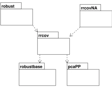
robustbase pcaPP rrcov
robust rrcovNA
Figure 2: Class diagram: structure of the framework and relation to other Rpackages.
thenew()function which will perform the necessary validity checks. We go one step further
and require that the new() function is not used directly but only through special functions
known in R as generating functions or as constructors in the conventional object oriented
programming languages. A constructor function has the same name as the corresponding class, takes the estimation options as parameters, organizes the necessary computations and
returns an object of the class containing the results of the computation. It can take as
a parameter also a control object which itself is an S4 object and contains the estimation
options. More details on the generating functions and their application for structuring the user interface can be found inRuckdeschelet al. (2009).
The main part of the framework is implemented in the packagerrcovbut it relies on code in
the packagesrobustbase and pcaPP(Filzmoser et al. 2009). The structure of the framework
and its relation to otherRpackages is shown in Figure2. The framework can be used by other
packages, like for example by robust (see Wang et al. 2008) or can be further extended. In
Figure2 a hypothetical package rrcovNA is shown, which could extend the available robust
multivariate methods with options for dealing with missing values.
In the rest of this section some object-oriented programming (OOP) concepts will be discussed which are essential for understanding the framework.
2.1. UML diagrams
Throughout this paper we exploit UML class diagrams to give a clear picture of the framework
and its components. UML stands forUnified Modeling Language—an object-oriented system
of notation which has evolved from previous works of Grady Booch, James Rumbaugh and Ivar Jacobson to become a tool accepted by the Object Management Group (OMG) as the
standard for modeling object-oriented programs (seeOMG 2009a,b). A class diagram models
the structure and contents of a system by depicting classes, packages, objects and the relations among them with the aim to increase the ease of understanding the considered application.
A class is denoted by a box with three compartments which contain the name, the attributes (slots) and operations (methods) of the class, respectively. The class name in italics indicates that the class is abstract. The bottom two compartments could be omitted or they can contain only the key attributes and operations which are useful for understanding the particular diagram. Each attribute is followed by its type and each operation—by the type of its return value. We use theRtypes like numeric,logical,vector,matrix, etc. but the type can be also a name of an S4 class.
Relationships between classes are denoted by lines or arrows with different form. The inher-itance relationship is depicted by a large empty triangular arrowhead pointing to the base class. Composition means that one class contains another one as a slot (not to be mistaken with the keyword “contains” signalling inheritance in R). This relation is represented by an arrow with a solid diamond on the side of the composed class. If a class “uses” another one or depends on it, the classes are connected by a dashed arrow (dependence relation).
Pack-ages can also be present in a class diagram—in our case they correspond more or less toR
packages—and are shown as tabbed boxes with the name of the package written in the tab (see Figure 2).
All UML diagrams of the framework were created with the open source UML toolArgoUML
(Robbins 1999; Robbins and Redmiles 2000) which is available for download from http: //argouml.tigris.org/.
2.2. Design patterns
Design patterns are usually defined as general solutions to recurring design problems and refer to both the description of a solution and an instance of that solution solving a particular problem. The current use of the term design patterns originates in the writings of the architect Christopher Alexander devoted to urban planning and building architecture (Alexanderet al.
1977) but it was brought to the software development community by the seminal book of
Gamma et al. (1995).
A design pattern can be seen as a template for how to solve a problem which can be used in many different situations. Object-oriented design patterns are about classes and the relation-ships between classes or objects at abstract level, without defining the final classes or objects of the particular application. In order to be usable, design patterns must be defined formally and the documentation, including a preferably evocative name, describes the context in which the pattern is used, the pattern structure, the participants and collaboration, thus presenting the suggested solution.
Design patterns are not limited to architecture or software development but can be applied in any domain where solutions are searched for. During the development of the here presented framework several design patterns were identified, which we prefer to call statistical design patterns. The first one was already described earlier in this section and captures the relations among a classical and one or more alternative robust multivariate estimators. Another can-didate is the control object encapsulating the estimation parameters and a third one is the factory-like construct which suggests selection of a robust estimation method and creation of the corresponding objects based on the data set characteristics (see Section 4.1). The formal description of these design patterns is beyond the scope of this work and we will limit the discussion to several examples.
2.3. Accessor methods
One of the major characteristics and advantages of object-oriented programming is the encap-sulation. Unfortunately real encapsulation (information hiding) is missing inR, but as far as the access to the member variables is concerned this could be mitigated by defining accessor methods (i.e., methods used to examine or modify the slots (member variables) of a class) and “advising” the users to use them instead of directly accessing the slots. The usual way of defining accessor functions inRis to use the same name as the name of the corresponding slot. For example for the slot athese are:
R> cc <- a(obj) R> a(obj) <- cc
In many cases this is not possible, because of conflicts with other existing functions. For example it is not possible to define an accessor function cov() for the slot cov of class Cov, since the functioncov()already exists in thebaseR. Also it is not immediately seen if a slot is “read only” or can be modified by the user (unfortunately, as already mentioned, every slot inRcan be modified by simply usingobj@a <- cc). Inrrcova notation was adopted, which
is usual in Java: the accessors are defined as getXxx()and setXxx()(if asetXxx()method
is missing, we are “not allowed” to change the slot). The use of accessor methods allows to
perform computations on demand (getMah(mcd)computes the Mahalanobis distances, stores
them into the object and returns them) or even have “virtual” slots which are not at all stored
in the object (e.g., getCorr(mcd) computes each time and returns the correlation matrix
without storing it).
2.4. Naming conventions
There is no agreed naming convention (coding rules) in R but to facilitate the framework
usage several simple rules are in order, following the recommended Sun’s Java coding style
(see http://java.sun.com/docs/codeconv/):
Class, function, method and variable names are alphanumeric, do not contain “-” or “.”
but rather use interchanging lower and upper case.
Class names start with an uppercase letter.
Methods, functions, and variables start with a lowercase letter.
Exceptions are functions returning an object of a given class (i.e., generating functions or constructors)—they have the same name as the class.
Variables and methods which are not intended to be seen by the user—i.e., private
members—start with “.”.
3. Example session
In this section we will introduce the base functionalities of the framework by an example session. First of all we have to load the packagerrcovwhich will cause all necessary packages to be loaded too. The framework includes many example data sets but here we will load only those which will be used throughout the following examples. For the rest of the paper it will be assumed that the package has been loaded already.
R> library("rrcov")
pcaPP 0.1-1 loaded
Scalable Robust Estimators with High Breakdown Point (version 0.5-03)
R> data("delivery")
R> delivery.x <- delivery[, 1:2] R> data("hbk")
R> hbk.x <- hbk[, 1:3]
Most of the multivariate statistical methods are based on estimates of multivariate location
and covariance, therefore these estimates play a central role in the framework. We will
start with computing the robust minimum covariance determinant estimate for the data
set delivery from the package robustbase. The data set (see Rousseeuw and Leroy 1987, Table 23, p. 155) contains delivery time data in 25 observations with 3 variables. The aim is to explain the time required to service a vending machine(Y)by means of the number of products
stocked (X1) and the distance walked by the route driver (X2). For this example we will
consider only the Xpart of the data set. After computing its robust location and covariance
matrix using the MCD method implemented in the function CovMcd() we can print the
results by calling the defaultshow() method on the returned object mcdas well as summary
information by the summary() method. The standard output contains the robust estimates
of location and covariance. The summary output contains additionally the eigenvalues of the covariance matrix and the robust distances of the data items (Mahalanobis type distances computed with the robust location and covariance instead of the sample ones).
R> mcd <- CovMcd(delivery.x) R> mcd
Call:
CovMcd(x = delivery.x)
-> Method: Minimum Covariance Determinant Estimator. Robust Estimate of Location:
n.prod distance 5.895 268.053
Robust Estimate of Covariance:
n.prod distance
n.prod 11.66 220.72
R> summary(mcd)
Call:
CovMcd(x = delivery.x)
Robust Estimate of Location: n.prod distance
5.895 268.053
Robust Estimate of Covariance:
n.prod distance
n.prod 11.66 220.72
distance 220.72 53202.65
Eigenvalues of covariance matrix:
[1] 53203.57 10.74 Robust Distances: [1] 1.6031 0.7199 1.0467 0.7804 0.2949 0.1391 1.4464 0.2321 [9] 60.8875 2.6234 9.8271 1.7949 0.3186 0.7526 1.1267 5.2213 [17] 0.1010 0.6075 1.3597 12.3162 2.3099 35.2113 1.1366 2.5625 [25] 0.4458 R> plot(mcd, which = "dd")
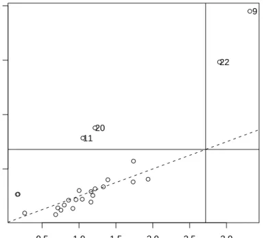
Now we will show one of the available plots by calling the plot() method—in Figure 3 the
Distance-Distance plot introduced byRousseeuw and van Zomeren(1991) is presented, which
plots the robust distances versus the classical Mahalanobis distances and allows to classify
the observations and identify the potential outliers. The description of this plot as well
as examples of more graphical displays based on the covariance structure will be shown in Section 4.1.
Apart from the demonstrated MCD method the framework provides many other robust es-timators of multivariate location and covariance, actually almost all of the well established estimates in the contemporary robustness literature. The most fascinating feature of the framework is that one will get the output and the graphs in the same format, whatever esti-mation method was used. For example the following code lines will compute the S estimates for the same data set and provide the standard and extended output (not shown here).
R> est <- CovSest(delivery.x, method = "bisquare") R> est
R> summary(est)
Nevertheless, this variety of methods could pose a serious hurdle for the novice and could be quite tedious even for the experienced user. Therefore a shortcut is provided too—the
function CovRobust() can be called with a parameter set specifying any of the available
estimation methods, but if this parameter set is omitted the function will decide on the basis of the data size which method to use. As we see in the example below, in this case it selects the Stahel-Donoho estimates. For details and further examples see Section 4.1.
● ● ● ● ● ● ● ● ● ● ● ● ● ● ● ● ● ● ● ● ● ● ● ● ● 0.5 1.0 1.5 2.0 2.5 3.0 2 4 6 8 Mahalanobis distance Rob ust distance 11 20 22 9 Distance−Distance Plot
Figure 3: Example plot of the robust against classical distances for the deliverydata set.
R> est <- CovRobust(delivery.x) R> est
Call:
CovSde(x = x, control = obj)
-> Method: Stahel-Donoho estimator Robust Estimate of Location:
n.prod distance 5.842 275.401
Robust Estimate of Covariance:
n.prod distance
n.prod 9.492 347.498
4. Robust multivariate methods
4.1. Multivariate location and scatter
The framework provides an almost complete set of estimators for multivariate location and scatter with high breakdown point. The first such estimator was proposed byStahel(1981a,b) andDonoho(1982) and it is recommended for small data sets, but the most widely used high
breakdown estimator is the minimum covariance determinant estimate (Rousseeuw 1985).
Several algorithms for computing the S estimators (Davies 1987) are provided (Ruppert 1992; Woodruff and Rocke 1994; Rocke 1996; Salibian-Barrera and Yohai 2006). The minimum volume ellipsoid (MVE) estimator (Rousseeuw 1985) is also included since it has some
desir-able properties when used as initial estimator for computing the S estimates (see Maronna
et al. 2006, p. 198). In the rest of this section the definitions of the different estimators of location and scatter will be briefly reviewed and the algorithms for their computation will be discussed. Further details can be found in the relevant references. The object model is presented and examples of its usage, as well as further examples of the graphical displays are given.
The minimum covariance determinant estimator and its computation
The MCD estimator for a data set{x1, . . . ,xn}in<p is defined by that subset{xi1, . . . ,xih}
of h observations whose covariance matrix has the smallest determinant among all possible
subsets of sizeh. The MCD location and scatter estimate TMCD and CMCD are then given
as the arithmetic mean and a multiple of the sample covariance matrix of that subset
TMCD = 1 h h X j=1 xij CM CD = cccfcsscf 1 h−1 h X j=1 (xij−TMCD)(xij−TMCD) > . (1)
The multiplication factors cccf (consistency correction factor) and csscf (small sample
cor-rection factor) are selected so that C is consistent at the multivariate normal model and
unbiased at small samples (seeButler et al. 1993;Croux and Haesbroeck 1999; Pison et al.
2002;Todorov 2008). A recommendable choice forhis b(n+p+ 1)/2cbecause then the BP of the MCD is maximized, but any integer h within the interval [(n+p+ 1)/2, n] can be chosen, seeRousseeuw and Leroy(1987). Here bzcdenotes the integer part of zwhich is not
less thanz. Ifh =nthen the MCD location and scatter estimate TMCD and CMCD reduce
to the sample mean and covariance matrix of the full data set.
The computation of the MCD estimator is far from being trivial. The naive algorithm would proceed by exhaustively investigating all subsets of sizehout ofnto find the subset with the smallest determinant of its covariance matrix, but this will be feasible only for very small data sets. Initially MCD was neglected in favor of MVE because the simple resampling algorithm was more efficient for MVE. Meanwhile several heuristic search algorithms (seeTodorov 1992; Woodruff and Rocke 1994;Hawkins 1994) and exact algorithms (Agull´o 1996) were proposed
but now a very fast algorithm due to Rousseeuw and Van Driessen (1999) exists and this
one approximation (T1,C1) of the MCD estimate of a data setX={x1, . . . ,xn} to the next one (T2,C2) with possibly lower determinant det(C2)≤det(C1) by computing the distances
d1, . . . , dn relative to (T1,C1), i.e.,
di= q
(xi−T1)>C1−1(xi−T1) (2)
and then computing (T2,C2) for those h observations which have smallest distances. “C” in C-step stands for “concentration” since we are looking for a more “concentrated” covariance
matrix with lower determinant. Rousseeuw and Van Driessen (1999) have proven a theorem
stating that the iteration process given by the C-step converges in a finite number of steps to a (local) minimum. Since there is no guarantee that the global minimum of the MCD objective function will be reached, the iteration must be started many times from different initial subsets, to obtain an approximate solution. The procedure is very fast for small data sets but to make it really “fast” also for large data sets several computational improvements are used.
initial subsets: It is possible to restart the iterations from randomly generated subsets of size h, but in order to increase the probability of drawing subsets without outliers,
p+ 1 points are selected randomly. These p+ 1 points are used to compute (T0,C0). Then the distances d1, . . . , dnare computed and sorted in increasing order. Finally the first h are selected to form the initialh−subsetH0.
reduced number of C-steps: The C-step involving the computation of the covariance matrix, its determinant and the relative distances, is the most computationally intensive part of the algorithm. Therefore instead of iterating to convergence for each initial subset only two C-steps are performed and the 10 subsets with lowest determinant are kept. Only these subsets are iterated to convergence.
partitioning: For large n the computation time of the algorithm increases mainly be-cause all ndistances given by Equation (2) have to be computed at each iteration. An improvement is to partition the data set into a maximum of say five subsets of approx-imately equal size (but not larger than say 300) and iterate in each subset separately. The ten best solutions for each data set are kept and finally only those are iterated on the complete data set.
nesting: Further decrease of the computational time can be achieved for data sets withn
larger than say 1500 by drawing 1500 observations without replacement and performing the computations (including the partitioning) on this subset. Only the final iterations are carried out on the complete data set. The number of these iterations depends on the actual size of the data set at hand.
The MCD estimator is not very efficient at normal models, especially ifh is selected so that maximal BP is achieved. To overcome the low efficiency of the MCD estimator, a reweighed version can be used. For this purpose a weightwi is assigned to each observationxi, defined aswi= 1 if (xi−TMCD)>C−MCD1 (xi−TMCD)≤χ2p,0.975and wi = 0 otherwise, relative to the
raw MCD estimates (TMCD,CMCD). Then the reweighted estimates are computed as TR = 1 ν n X i=1 wixi, CR = cr.ccfcr.sscf 1 ν−1 n X i=1 wi(xi−TR)(xi−TR)>, (3)
whereν is the sum of the weights, ν =Pn
i=1wi. Again, the multiplication factors cr.ccf and
cr.sscf are selected so that CR is consistent at the multivariate normal model and unbiased
at small samples (see Pison et al. 2002; Todorov 2008, and the references therein). These
reweighted estimates (TR,CR) which have the same breakdown point as the initial (raw)
estimates but better statistical efficiency are computed and used by default.
The minimum volume ellipsoid estimates
The minimum volume ellipsoid estimator searches for the ellipsoid of minimal volume con-taining at least half of the points in the data setX. Then the location estimate is defined as the center of this ellipsoid and the covariance estimate is provided by its shape. Formally the estimate is defined as theseTMVE,CMVE that minimize det(C) subject to
#{i: (xi−T)>C−1(xi−T)≤c2} ≥ n+p+ 1 2 , (4)
where # denotes the cardinality. The constantc is chosen as χ2p,0.5.
The search for the approximate solution is made over ellipsoids determined by the covariance
matrix of p+ 1 of the data points and by applying a simple but effective improvement of
the sub-sampling procedure as described in Maronna et al. (2006), p. 198. Although there
exists no formal proof of this improvement (as for MCD and LTS), simulations show that it can be recommended as an approximation of the MVE. The MVE was the first popular high breakdown point estimator of location and scatter but later it was replaced by the MCD, mainly because of the availability of an efficient algorithm for its computation (Rousseeuw and Van Driessen 1999). Recently the MVE gained importance as initial estimator for S estimation because of its small maximum bias (seeMaronnaet al. 2006, Table 6.2, p. 196).
The Stahel-Donoho estimator
The first multivariate equivariant estimator of location and scatter with high breakdown point
was proposed by Stahel (1981a,b) and Donoho (1982) but became better known after the
analysis of Maronna and Yohai (1995). For a data set X= {x1, . . . ,xn} in <p it is defined
as a weighted mean and covariance matrix of the form given by Equation (3) where the
weightwi of each observation is inverse proportional to the “outlyingness” of the observation. Let the univariate outlyingness of a pointxi with respect to the data set X along a vector a∈ <p,||a|| 6=0 be given by
r(xi,a) =
|x>a−m(a>X)|
s(a>X) i= 1, . . . , n (5) where (a>X) is the projection of the data setXonaand the functionsm() ands() are robust univariate location and scale statistics, for example the median and MAD, respectively. Then
the multivariate outlyingness ofxi is defined by
ri =r(xi) = max
a r(xi,a). (6)
The weights are computed by wi = w(ri) where w(r) is a nonincreasing function of r and
w(r) andw(r)r2 are bounded. Maronna and Yohai (1995) use the weights
w(r) = min 1,c t 2 (7)
withc=qχ2p,β and β = 0.95, that are known in the literature as “Huber weights”.
Exact computation of the estimator is not possible and an approximate solution is found
by subsampling a large number of directions a and computing the outlyingness measures
ri, i= 1, . . . , n for them. For each subsample ofp points the vector ais taken as the norm 1 vector orthogonal to the hyperplane spanned by these points. It has been shown by simulations (Maronnaet al. 2006) that one step reweighting does not improve the estimator.
Orthogonalized Gnanadesikan/Kettenring
The MCD estimator and all other known affine equivariant high-breakdown point estimates are solutions to a highly non-convex optimization problem and as such pose a serious compu-tational challenge. Much faster estimates with high breakdown point can be computed if one gives up the requirements of affine equivariance of the covariance matrix. Such an algorithm
was proposed byMaronna and Zamar (2002) which is based on the very simple robust
bivari-ate covariance estimator sjk proposed by Gnanadesikan and Kettenring (1972) and studied
by Devlinet al. (1981). For a pair of random variables Yj and Yk and a standard deviation function σ(), sjk is defined as sjk = 1 4 σ Yj σ(Yj) + Yk σ(Yk) 2 −σ Yj σ(Yj) − Yk σ(Yk) 2! . (8)
If a robust function is chosen forσ() then sjk is also robust and an estimate of the covariance matrix can be obtained by computing each of its elements sjk for each j = 1, . . . , p and
k = 1, . . . , p using Equation (8). This estimator does not necessarily produce a positive
definite matrix (although symmetric) and it is not affine equivariant. Maronna and Zamar
(2002) overcome the lack of positive definiteness by the following steps:
Defineyi=D−1xi, i= 1, . . . , nwithD= diag(σ(X1), . . . , σ(Xp)) whereXl, l= 1, . . . , p are the columns of the data matrix X ={x1, . . . ,xn}. Thus a normalized data matrix
Y ={y1, . . . ,yn} is computed.
Compute the matrix U = (ujk) as ujk =sjk =s(Yj, Yk) ifj 6=kor ujk = 1 otherwise. Here Yl, l = 1, . . . , pare the columns of the transformed data matrix Y and s(., .) is a robust estimate of the covariance of two random variables like the one in Equation (8).
Obtain the “principal component decomposition” of Y by decomposing U = EΛE>
whereΛ is a diagonal matrixΛ= diag(λ1, . . . , λp) with the eigenvaluesλj ofU and E is a matrix with columns the eigenvalues ej of U.
Define zi = E>yi = E>D−1xi and A = DE. Then the estimator of Σ is COGK =
AΓA>whereΓ= diag(σ(Zj)2), j= 1, . . . , pand the location estimator isTOGK =Am where m=m(zi) = (m(Z1), . . . , m(Zp)) is a robust mean function.
This can be iterated by computing COGK and TOGK forZ ={z1, . . . ,zn} obtained in the last step of the procedure and then transforming back to the original coordinate system.
Simulations (Maronna and Zamar 2002) show that iterations beyond the second did not lead
to improvement.
Similarly as for the MCD estimator a one-step reweighting can be performed using Equa-tions (3) but the weights wi are based on the 0.9 quantile of the χ2p distribution (instead of 0.975) and the correction factors cr.ccf and cr.sscf are not used.
In order to complete the algorithm we need a robust and efficient location function m() and
scale function σ(), and one proposal is given in Maronna and Zamar (2002). Further, the
robust estimate of covariance between two random vectors s() given by Equation (8) can be replaced by another one. In the framework two such functions are predefined but the user can provide as a parameter an own function.
S estimates
S estimators of µ and Σwere introduced by Davies (1987) and further studied by Lopuha¨a
(1989) (see alsoRousseeuw and Leroy 1987, p. 263). For a data set ofp-variate observations
{x1, . . . ,xn} an S estimate (T,C) is defined as the solution of σ(d1, . . . , dn) = min where
di = (x−T)>C−1(x−T) and det(C) = 1. Here σ = σ(z) is the M-scale estimate of a data setz ={z1, . . . , zn} defined as the solution of 1nΣρ(z/σ) =δ where ρ is nondecreasing,
ρ(0) = 0 and ρ(∞) = 1 andδ∈(0,1). An equivalent definition is to find the vectorT and a positive definite symmetric matrixCthat minimize det(C) subject to
1 n n X i=1 ρ(di) =b0 (9)
with the above di and ρ.
As shown by Lopuha¨a (1989) S estimators have a close connection to the M estimators and
the solution (T,C) is also a solution to an equation defining an M estimator as well as a weighted sample mean and covariance matrix:
dji = [(xi−T(j−1))>(C(j−1))−1(x−T(j−1))]1/2 T(j) = Σw(d (j) i )xi Σw(d(ij)) C(j) = Σw(d (j) i )(xi−T(j))(xi−T(j)) > Σw(d(ij)) (10)
The framework implements the S estimates in the classCovSest and provides four different
algorithms for their computation.
1. SURREAL: This algorithm was proposed by Ruppert (1992) as an analog to the algo-rithm proposed by the same author for computing S estimators of regression.
2. Bisquare S estimation with HBDP start: S estimates with the biweight ρ function can be obtained using the Equations (10) by a reweighted sample covariance and reweighted
sample mean algorithm as described inMaronna et al. (2006). The preferred approach
is to start the iteration from a bias-robust but possibly inefficient estimate which is
computed by some form of sub-sampling. SinceMaronnaet al. (2006) have shown that
the MVE has smallest maximum bias (Table 6.2, p. 196) it is recommended to use it as initial estimate.
3. Rocke type S estimates: InRocke(1996) it is shown that S estimators in high dimensions can be sensitive to outliers even if the breakdown point is set to 50%. Therefore they
propose a modified ρ function called translated biweight (or t-biweight) and replace
the standardization step given in Equation (9) with a standardization step consisting
of equating the median of ρ(di) with the median under normality. The estimator is
shown to be more outlier resistant in high dimensions than the typical S estimators. The specifics of the iteration are given inRocke and Woodruff(1996), see alsoMaronna
et al. (2006). As starting values for the iteration any of the available methods in the framework can be used. The recommended (and consequently the default) one is the
MVE estimator computed by CovMve().
4. Fast S estimates: Salibian-Barrera and Yohai (2006) proposed a fast algorithm for
re-gression S estimates similar to the FAST-LTS algorithm ofRousseeuw and Van Driessen
(2006) and borrowing ideas from the SURREAL algorithm of Ruppert (1992).
Simi-larly, the FAST-S algorithm for multivariate location and scatter is based on modifying each candidate to improve the S-optimality criterion thus reducing the number of the necessary sub-samples required to achieve desired high breakdown point with high prob-ability.
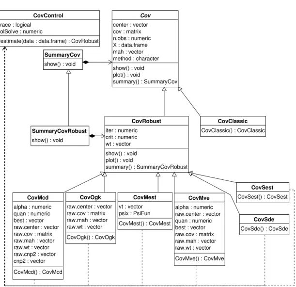
Object model for robust location and scatter estimation
The object model for the S4 classes and methods implementing the different multivariate
location and scatter estimators follows the proposed class hierarchy given in Section 2and is presented in Figure 4.
The abstract class Covserves as a base class for deriving all classes representing classical and robust location and scatter estimation methods. It defines the common slots and the
cor-responding accessor methods, provides implementation for the general methods like show(),
plot() and summary(). The slots of Cov hold some input or default parameters as well as the results of the computations: the location, the covariance matrix and the distances. The show()method presents brief results of the computations and thesummary()method returns
an object of classSummaryCov which has its own show() method. As in the other sections
of the framework these slots and methods are defined and documented only once in this base class and can be used by all derived classes. Whenever new data (slots) or functionality (methods) are necessary, they can be defined or redefined in the particular class.
The classical location and scatter estimates are represented by the class CovClassic which
inherits directly from Cov (and uses all slots and methods defined there). The function
CovClassic()serves as a constructor (generating function) of the class. It can be called by
providing a data frame or matrix. As already demonstrated in Section3the methodsshow()
Cov show() : void plot() : void summary() : SummaryCov center : vector cov : matrix n.obs : numeric X : data.frame mah : vector method : character CovMcd CovMcd() : CovMcd alpha : numeric quan : numeric best : vector raw.center : vector raw.cov : matrix raw.mah : vector raw.wt : vector raw.cnp2 : vector cnp2 : vector CovRobust show() : void plot() : void summary() : SummaryCovRobust iter : numeric crit : numeric wt : vector CovMest CovMest() : CovMest vt : vector psix : PsiFun CovOgk CovOgk() : CovOgk raw.center : vector raw.cov : matrix raw.mah : vector raw.wt : vector SummaryCov show() : void SummaryCovRobust show() : void CovControl
restimate(data : data.frame) : CovRobust trace : logical tolSolve : numeric CovClassic CovClassic() : CovClassic CovMve CovMve() : CovMve alpha : numeric raw.center : vector quan : numeric best : vector raw.cov : matrix raw.mah : vector raw.wt : vector CovSest CovSest() : CovSest CovSde CovSde() : CovSde
Figure 4: Object model for robust location and scatter estimation.
diagnostic plots which are shown in one of the next sections. The accessor functions like getCenter(),getCov(), etc. are used to access the corresponding slots.
Another abstract class, CovRobust is derived from Cov, which serves as a base class for all robust location and scatter estimators.
The classes representing robust estimators likeCovMcd,CovMve, etc. are derived fromCovRobust and provide implementation for the corresponding methods. Each of the constructor functions CovMcd(),CovMve(),CovOgk(),CovMest() andCovSest() performs the necessary computa-tions and returns an object of the class containing the results. Similarly as theCovClassic() function, these functions can be called either with a data frame or a numeric matrix.
Controlling the estimation options
Although the different robust estimators of multivariate location and scatter have some con-trolling options in common, like the tracing flagtraceor the numeric tolerance tolSolveto
CovControlMcd
restimate(data : data.frame) : CovMcd alpha : numeric
nsamp : numeric seed : vector use.correction : logical
CovControl
restimate(data : data.frame) : CovRobust trace : logical
tolSolve : numeric
CovControlMest
restimate(data : data.frame) : CovMest r : numeric
arp : numeric eps : double maxiter : integer
CovControlOgk
restimate(data : data.frame) : CovOgk mrob() : double vrob() : double niter : numeric beta : numeric smrob : character svrob : character CovControlMve
restimate(data : data.frame) : CovMve alpha : double
nsamp : integer seed : vector
CovControlSest
restimate(data : data.frame) : CovSest bdp : double
nsamp : integer seed : vector method : character
CovControlSde
restimate(data : data.frame) : CovSde nsamp : numeric maxres : numeric tune : numeric eps : numeric prob : numeric seed : vector
Figure 5: Object model of the control classes for robust location and scatter estimation.
be used for inversion (solve) of the covariance matrix in mahalanobis(), each of them has
more specific options. For example, the MCD and MVE estimators (CovMcd()andCovMve())
can specify alphawhich controls the size of the subsets over which the determinant (the vol-ume of the ellipsoid) is minimized. The allowed values are between 0.5 and 1 and the default is 0.5. Similarly, these estimators have parameters nsampfor the number of subsets used for initial estimates andseed for the initial seed for R’s random number generator while the M
and S estimators (CovMest and CovSest) have to specify the required breakdown point
(al-lowed values between (n−p)/(2·n) and 1 with default 0.5) as well as the asymptotic rejection point, i.e., the fraction of points receiving zero weight (Rocke and Woodruff 1996).
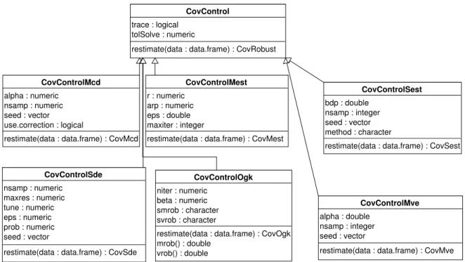
These parameters can be passed directly to the corresponding constructor function but ad-ditionally there exists the possibility to use a control object serving as a container for the
parameters. The object model for the control objects shown in Figure5follows the proposed
class hierarchy—there is a base classCovControl which holds the common parameters and
from this class all control classes holding the specific parameters of their estimators are de-rived. These classes have only a constructor function for creating new objects and a method restimate() which takes a data frame or a matrix, calls the corresponding estimator to perform the calculations and returns the created class with the results.
Apart from providing a structured container for the estimation parameters this class hierarchy has the following additional benefits:
the parameters can be passed easily to another multivariate method, for example the
principal components analysis based on a covariance matrix PcaCov()(see Section4.2) can take a control object which will be used to estimate the desired covariance (or correlation) matrix. In the following example a control object holding the parameters
for S estimation will be created and then PcaCov()will be called with this object.
R> control <- CovControlSest(method = "biweight") R> PcaCov(hbk.x, cov.control = control)
Call:
PcaCov(x = hbk.x, cov.control = control) Standard deviations: [1] 1.409393 1.262539 1.142856 Loadings: PC1 PC2 PC3 X1 -0.5256781 0.74354209 -0.4132888 X2 -0.6219784 -0.66738398 -0.4095626 X3 -0.5803494 0.04175861 0.8132963
the class hierarchy of the control objects allows to handle different estimator objects using a uniform interface thus leveraging one of the most important features of the object-oriented programming, the polymorphism. In the following example we create a list containing different control objects and then viasapplywe call the generic function restimate()on each of the objects in the list. The outcome will be a list containing the objects resulting from these calls (all are derived from CovRobust). This looping over the different estimation methods is very useful for implementing simulation studies.
R> cc <- list(CovControlMcd(), CovControlMest(), CovControlOgk(), + CovControlSest(), CovControlSest(method = "rocke"))
R> clist <- sapply(cc, restimate, x = delivery.x) R> sapply(clist, data.class)
[1] "CovMcd" "CovMest" "CovOgk" "CovSest" "CovSest"
R> sapply(clist, getMeth)
[1] "Minimum Covariance Determinant Estimator." [2] "M-Estimates"
[3] "Orthogonalized Gnanadesikan-Kettenring Estimator" [4] "S-estimates: S-FAST"
[5] "S-estimates: Rocke type"
A generalized function for robust location and covariance estimation: CovRobust() The provided variety of estimation methods, each of them with different parameters as well as the object models described in the previous sections can be overwhelming for the user, especially for the novice who does not care much about the technical implementation of the framework. Therefore a function is provided which gives a quick access to the robust estimates of location and covariance matrix. This function is loosely modeled around the
concrete objects of derived classes and returns the result over a base class interface. The class CovRobustis abstract (defined as VIRTUAL) and no objects of it can be created but any of the classes derived from CovRobust, such as CovMcd orCovOgk, can act as an object of class CovRobust. The function CovRobust() which is technically not a constructor function can return an object of any of the classes derived fromCovRobust according to the user request. This request can be specified in one of three forms:
If only a data frame or matrix is provided and the control parameter is omitted, the
function decides which estimate to apply according to the size of the problem at hand. If there are less than 1000 observations and less than 10 variables or less than 5000 observations and less than 5 variables, Stahel-Donoho estimator will be used. Otherwise, if there are less than 50000 observations, either bisquare S estimates (in case of less than 10 variables) or Rocke type S estimates (for 10 to 20 variables) will be used. In both cases the S iteration starts at the initial MVE estimate. And finally, if there are more than 50000 observations and/or more than 20 variables the Orthogonalized Quadrant
Correlation estimator (CovOgk with the corresponding parameters) is used. This is
illustrated by the following example.
R> getMeth(CovRobust(matrix(rnorm(40), ncol = 2)))
[1] "Stahel-Donoho estimator"
R> getMeth(CovRobust(matrix(rnorm(16000), ncol = 8)))
[1] "S-estimates: bisquare"
R> getMeth(CovRobust(matrix(rnorm(20000), ncol = 10)))
[1] "S-estimates: Rocke type"
R> getMeth(CovRobust(matrix(rnorm(2e+05), ncol = 2)))
[1] "Orthogonalized Gnanadesikan-Kettenring Estimator"
The simplest way to choose an estimator is to provide a character string with the name
of the estimator—one of"mcd","ogk","m","s-fast","s-rocke", etc.
R> getMeth(CovRobust(matrix(rnorm(40), ncol = 2), control = "rocke"))
[1] "S-estimates: Rocke type"
If it is necessary to specify also some estimation parameters, the user can create a
control object (derived from CovControl) and pass it to the function together with the data. For example to compute the OGK estimator using the median absolute deviation (MAD) as a scale estimate and the quadrant correlation (QC) as a pairwise correlation
estimate we create a control objectctrlpassing the parameterss_madand s_qcto the
constructor function and then callCovRobust with this object. The last command line
illustrates the accessor method for getting the correlation matrix of the estimate as well as a nice formatting method for covariance matrices.
R> data("toxicity")
R> ctrl <- CovControlOgk(smrob = "s_mad", svrob = "qc") R> est <- CovRobust(toxicity, ctrl)
R> round(getCenter(est), 2)
toxicity logKow pKa ELUMO Ecarb Emet RM IR
-0.20 1.40 0.40 4.01 16.99 3.25 35.41 1.46
Ts P
41.72 1.46
R> as.dist(round(getCorr(est), 2))
toxicity logKow pKa ELUMO Ecarb Emet RM IR Ts
logKow 0.72 pKa -0.41 -0.13 ELUMO -0.26 0.23 0.33 Ecarb 0.19 0.68 0.48 0.61 Emet 0.56 0.87 0.16 0.09 0.68 RM 0.37 0.81 0.35 0.30 0.90 0.88 IR -0.20 0.17 0.41 0.18 0.58 0.22 0.59 Ts -0.57 -0.49 0.45 -0.17 -0.04 -0.27 0.00 0.70 P -0.20 0.17 0.41 0.18 0.58 0.22 0.59 1.00 0.70
Visualization of the results
The default plot accessed through the method plot() of class CovRobust is the
Distance-Distance plot introduced byRousseeuw and van Zomeren(1991). An example of this graph,
which plots the robust distances versus the classical Mahalanobis distances is shown in Fig-ure3. The dashed line represents the points for which the robust and classical distances are equal. The horizontal and vertical lines are drawn at valuesx=y=
q
χ2p,0.975. Points beyond these lines can be considered as outliers and are identified by their labels.
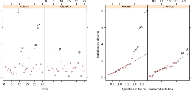
The other available plots are accessible either interactively or through thewhichparameter of theplot()method. The left panel of Figure6shows an example of the distance plot in which robust and classical Mahalanobis distances are shown in parallel panels. The outliers have large robust distances and are identified by their labels. The right panel of Figure 6 shows a Quantile-Quantile comparison plot of the robust and the classical Mahalanobis distances versus the square root of the quantiles of the chi-squared distribution.
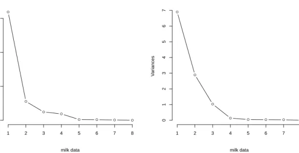
The next plot shown in Figure7presents a scatter plot of the data on which the 97.5% robust and classical confidence ellipses are superimposed. Currently this plot is available only for bivariate data. The observations with distances larger thanqχ2
p,0.975 are identified by their subscript. In the right panel of Figure7ascreeplotof themilkdata set is shown, presenting the robust and classical eigenvalues.
Distance Plot Index Mahalanobis distance 0 2 4 6 8 0 5 10 15 20 25 ● ●●● ● ● ● ● ● ● ● ● ● ●● ● ● ● ● ● ● ● ● ● ● 11 20 22 9 Robust 0 5 10 15 20 25 ● ● ● ●● ● ● ● ● ● ● ● ● ● ● ● ● ● ● ● ● ● ● ● ● 22 9 Classical Chi−Square QQ−Plot
Quantiles of the chi−squared distribution
Mahalanobis distance 0 2 4 6 8 0.5 1.0 1.5 2.0 2.5 ● ●●●● ●●●● ●●●● ●●●● ●●● ● ● ● ● ● 11 20 22 9 Robust 0.5 1.0 1.5 2.0 2.5 ● ●● ●●●●● ●●●●● ●●●●●● ● ● ●● ● ● 22 9 Classical
Figure 6: Distance plot and Chi-square Q-Q plot of the robust and classical distances.
● ● ● ● ● ● ● ● ● ● ● ● ● ● ● ● ● ● ● ● ● ● ● ● ● −10 0 10 20 30 −500 0 500 1000 1500 11 20 22 9 Tolerance ellipse (97.5%) ● robust classical 1 2 3 4 5 6 7 8 0 5 10 15 Index Eigen v alues ● robust classical ● ● ● ● ● ● ● ● Scree plot
Figure 7: Robust and classical tolerance ellipse for thedeliverydata and robust and classical screeplot for the milk data.
R> data("milk")
R> usr <- par(mfrow = c(1, 2))
R> plot(CovMcd(delivery[, 1:2]), which = "tolEllipsePlot", classic = TRUE) R> plot(CovMcd(milk), which = "screeplot", classic = TRUE)
4.2. Principal component analysis
Principal component analysis is a widely used technique for dimension reduction achieved
by finding a smaller number q of linear combinations of the originally observed p variables
and retaining most of the variability of the data. Thus PCA is usually aiming at a graphical representation of the data in a lower-dimensional space. The classical approach to PCA mea-sures the variability through the empirical variance and is essentially based on computation of eigenvalues and eigenvectors of the sample covariance or correlation matrix. Therefore the results may be extremely sensitive to the presence of even a few atypical observations in the data. These discrepancies will carry over to any subsequent analysis and to any graphical display related to the principal components such as the biplot.
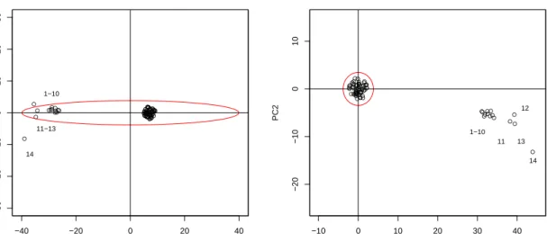
The following example in Figure8illustrates the effect of outliers on the classical PCA. The
data set hbk from the package robustbase consists of 75 observations in 4 dimensions (one
response and three explanatory variables) and was constructed by Hawkins, Bradu and Kass
in 1984 for illustrating some of the merits of a robust technique (see Rousseeuw and Leroy
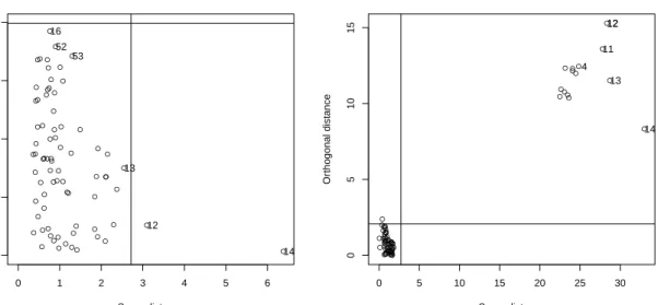
1987). The first 10 observations are bad leverage points, and the next four points are good leverage points (i.e., theirx are outlying, but the corresponding y fit the model quite well). We will consider only the X-part of the data. The left panel shows the plot of the scores on the first two classical principal components (the first two components account for more than 98% of the total variation). The outliers are identified as separate groups, but the regular points are far from the origin (where the mean of the scores should be located). Furthermore, the ten bad leverage points 1–10 lie within the 97.5% tolerance ellipse and influence the classical estimates of location and scatter. The right panel shows the same plot based on robust estimates. We see that the estimate of the center is not shifted by the outliers and these outliers are clearly separated by the 97.5% tolerance ellipse.
● ● ● ●● ●●●●● ● ● ● ● ● ●●●● ●●●●● ● ● ● ●●●● ● ● ● ●● ● ● ● ● ●● ● ●● ● ● ● ● ● ●● ● ● ● ● ● ● ●● ●●● ●●●●●●●●●●●● −40 −20 0 20 40 −30 −20 −10 0 10 20 30 Classical PC1 PC2 1−10 14 11−13 ● ●●●● ● ● ● ● ● ● ● ● ● ● ● ● ● ● ● ● ● ● ● ● ● ● ● ● ●● ● ● ● ● ● ● ● ● ● ● ● ● ● ● ●●●● ● ● ● ● ● ● ● ● ● ● ● ● ● ● ● ● ●● ●● ●● ● ● ● ● −10 0 10 20 30 40 −20 −10 0 10 Robust (MCD) PC1 PC2 1−10 11 12 13 14
Figure 8: Plot of the first two principal components of the Hawkins, Bradu and Kass data set: classical and robust.
PCA was probably the first multivariate technique subjected to robustification, either by simply computing the eigenvalues and eigenvectors of a robust estimate of the covariance matrix or directly by estimating each principal component in a robust manner. Different approaches to robust PCA are briefly presented in the next subsections with the emphasis on those methods which are available in the framework. Details about the methods and algorithms can be found in the corresponding references. The object model is described and examples are given.
PCA based on robust covariance matrix (MCD, OGK, MVE, etc.)
The most straightforward and intuitive method to obtain robust PCA is to replace the classical estimates of location and covariance by their robust analogues. In the earlier works M estima-tors of location and scatter were used for this purpose (seeDevlinet al.1981;Campbell 1980) but these estimators have the disadvantage of low breakdown point in high dimensions. To
cope with this problemNaga and Antille (1990) used the MVE estimator andTodorov et al.
(1994b) used the MCD estimator. Croux and Haesbroeck(2000) investigated the properties of the MCD estimator and computed its influence function and efficiency.
The package stats in base R contains the function princomp() which performs a principal
components analysis on a given numeric data matrix and returns the results as an object
of S3 class princomp. This function has a parameter covmat which can take a covariance
matrix, or a covariance list as returned bycov.wt, and if supplied, it is used rather than the covariance matrix of the input data. This allows to obtain robust principal components by
supplying the covariance matrix computed bycov.mveorcov.mcd from the packageMASS.
One could ask why is it then necessary to include such type of function in the framework (since it already exists in the base package). The essential value added of the framework, apart from implementing many new robust multivariate methods is the unification of the interfaces by leveraging the object orientation provided by theS4 classes and methods. The
function PcaCov() computes robust PCA by replacing the classical covariance matrix with
one of the robust covariance estimators available in the framework—MCD, OGK, MVE, M, S
or Stahel-Donoho, i.e., the parametercov.control can be any object of a class derived from
the base classCovControl. This control class will be used to compute a robust estimate of
the covariance matrix. If this parameter is omitted, MCD will be used by default. Of course any newly developed estimator following the concepts of the framework can be used as input to the functionPcaCov().
Projection pursuit methods
The second approach to robust PCA usesprojection pursuit (PP) and calculates directly the
robust estimates of the eigenvalues and eigenvectors. Directions are seeked for, which max-imize the variance (classical PCA) of the data projected onto them. Replacing the variance with a robust measure of spread yields robust PCA. Such a method was first introduced by Li and Chen (1985) using an M estimator of scale Sn as a projection index (PI). They showed that the PCA estimates inherit the robustness properties of the scale estimator Sn. Unfortunately, in spite of the good statistical properties of the method, the algorithm they proposed was too complicated to be used in practice. A more tractable algorithm in these
lines was first proposed byCroux and Ruiz-Gazen (1996) and later improved by Croux and
a new improved version was proposed by Croux et al. (2007). The latter two algorithms
are available in the package pcaPP (see Filzmoser et al. 2009) as functions PCAproj() and
PCAgrid().
In the framework these methods are represented by the classesPcaProjand PcaGrid. Their
generating functions provide simple wrappers around the original functions frompcaPP and
return objects of the corresponding class, derived fromPcaRobust.
A major advantage of the PP-approach is that it searches for the eigenvectors consecutively and in case of high-dimensional data when we are interested in only the first one or two prin-cipal components this results in reduced computational time. Even more, the PP-estimates cope with the main drawback of the covariance-based estimates—they can be computed for data matrices with more variables than observations.
Hubert method (ROBPCA)
The PCA method proposed byHubert et al. (2005) tries to combine the advantages of both
approaches—the PCA based on a robust covariance matrix and PCA based on projection pursuit. A brief description of the algorithm follows, for details see the relevant references (Hubertet al. 2008).
Letndenote the number of observations, andpthe number of original variables in the input
data matrixX. The ROBPCA algorithm finds a robust centerm of the data and a loading
matrixPof dimensionp×k. Its columns are orthogonal and define a new coordinate system. The scoresT, an n×kmatrix, are the coordinates of the centered observations with respect to the loadings:
T= (X−1m>)P (11)
where1is a column vector with allncomponents equal to 1. The ROBPCA algorithm yields
also a robust covariance matrix (often singular) which can be computed as
S=PLP> (12)
whereL is the diagonal matrix with the eigenvalues l1, . . . , lk. This is done in the following three main steps:
Step 1: The data are preprocessed by reducing their data space to the subspace spanned by thenobservations. This is done by singular value decomposition of the input data matrix. As a result the data are represented in a space whose dimension isrank(X), being at most
n−1 without loss of information.
Step 2: In this step a measure of outlyingness is computed for each data point. For this purpose the data points are projected on the n(n−1)/2 univariate directions through each
two points. If n is too large, maxdir directions are chosen at random (maxdir defaults to
250 but can be changed by the user). On every direction the univariate MCD estimator of location and scale is computed and the standardized distance to the center is measured. The largest of these distances (over all considered directions) is the outlyingness measure of the
data point. Theh data points with smallest outlyingness measure are used to compute the
covariance matrixΣh and to select the numberk of principal components to retain. This is
done by findingksuch thatlk/l1≥10−3 and Σkj=1lj/Σrj=1lj ≥0.8. Alternatively the number of principal componentsk can be specified by the user after inspecting the scree plot.
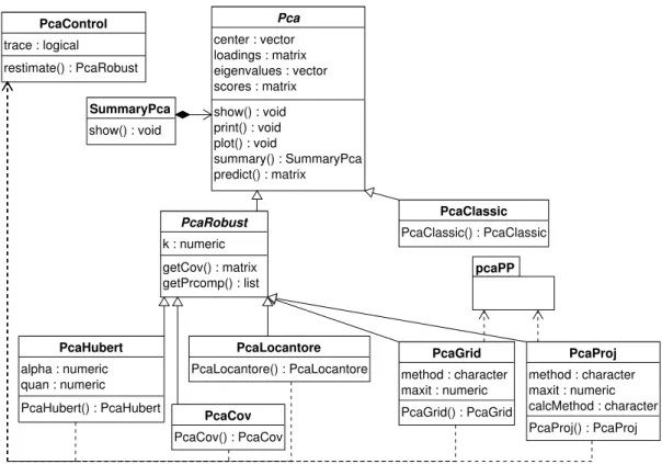
Pca show() : void print() : void plot() : void summary() : SummaryPca predict() : matrix center : vector loadings : matrix eigenvalues : vector scores : matrix PcaClassic PcaClassic() : PcaClassic PcaRobust getCov() : matrix getPrcomp() : list k : numeric PcaHubert PcaHubert() : PcaHubert alpha : numeric quan : numeric PcaGrid PcaGrid() : PcaGrid method : character maxit : numeric PcaProj PcaProj() : PcaProj method : character maxit : numeric calcMethod : character PcaControl restimate() : PcaRobust trace : logical pcaPP SummaryPca show() : void PcaLocantore PcaLocantore() : PcaLocantore PcaCov PcaCov() : PcaCov
Figure 9: Object model for robust Principal Component Analysis.
Step 3: The data points are projected on the k-dimensional subspace spanned by the k
eigenvectors corresponding to the largestk eigenvalues of the matrix Σh. The location and scatter of the projected data are computed using the reweighted MCD estimator, and the eigenvectors of this scatter matrix yield the robust principal components.
Spherical principal components (SPC)
The spherical principal components procedure was first proposed byLocantore et al. (1999) as a method for functional data analysis. The idea is to perform classical PCA on the data, projected onto a unit sphere. The estimates of the eigenvectors are consistent if the data are elliptically distributed (see Boente and Fraiman 1999) and the procedure is extremely fast.
Although not much is known about the efficiency of this method, the simulations ofMaronna
(2005) show that it has very good performance. If each coordinate of the data is normalized using some kind of robust scale, like for example the MAD, and then SPC is applied, we obtain “elliptical PCA”, but unfortunately this procedure is not consistent.
Object model for robust PCA and examples
The object model for the S4 classes and methods implementing the principal component
analysis methods follows the proposed class hierarchy given in Section 2 and is presented in Figure9.
robust principal components analysis methods. It defines the common slots and the
corre-sponding accessor methods, provides implementation for the general methods like show(),
plot(),summary() and predict(). The slots ofPca hold some input or default parameters like the requested number of components as well as the results of the computations: the
eigenvalues, the loadings and the scores. The show() method presents brief results of the
computations, and the predict() method projects the original or new data to the space
spanned by the principal components. It can be used either with new observations or with
the scores (if no new data are provided). Thesummary() method returns an object of class
SummaryPca which has its own show() method. As in the other sections of the framework these slots and methods are defined and documented only once in this base class and can be used by all derived classes. Whenever new information (slots) or functionality (methods) are necessary, they can be defined or redefined in the particular class.
Classical principal component analysis is represented by the classPcaClassicwhich inherits
directly fromPca(and uses all slots and methods defined there). The functionPcaClassic()
serves as a constructor (generating function) of the class. It can be called either by providing a data frame or matrix or a formula with no response variable, referring only to numeric
variables. Let us consider the following simple example with the data set hbk from the
packagerobustbase. The code line
R> PcaClassic(hbk.x)
can be rewritten as (and is equivalent to) the following code line using the formula interface
R> PcaClassic(~ ., data = hbk.x)
The functionPcaClassic()performs the standard principal components analysis and returns
an object of the classPcaClassic.
R> pca <- PcaClassic(~., data = hbk.x) R> pca Call: PcaClassic(formula = ~., data = hbk.x) Standard deviations: [1] 14.7024532 1.4075073 0.9572508 Loadings: PC1 PC2 PC3 X1 -0.2398767 0.1937359 -0.95127577 X2 -0.5547042 -0.8315255 -0.02947174 X3 -0.7967198 0.5206071 0.30692969 R> summary(pca) Call: PcaClassic(formula = ~., data = hbk.x)
Importance of components: PC1 PC2 PC3 Standard deviation 14.7025 1.40751 0.95725 Proportion of Variance 0.9868 0.00904 0.00418 Cumulative Proportion 0.9868 0.99582 1.00000 R> plot(pca) R> getLoadings(pca) PC1 PC2 PC3 X1 -0.2398767 0.1937359 -0.95127577 X2 -0.5547042 -0.8315255 -0.02947174 X3 -0.7967198 0.5206071 0.30692969
Theshow() method displays the standard deviations of the resulting principal components,
the loadings and the original call. The summary() method presents the importance of the
calculated components. The plot() draws a PCA diagnostic plot which is shown and
de-scribed later. The accessor functions like getLoadings(), getEigenvalues(), etc. are used
to access the corresponding slots, andpredict() is used to rotate the original or new data
to the space of the principle components.
Another abstract class, PcaRobust is derived from Pca, which serves as a base class for all robust principal components methods. The classes representing robust PCA methods like PcaHubert, PcaLocantore, etc. are derived from PcaRobust and provide implementation
for the corresponding methods. Each of the constructor functions PcaCov(), PcaHubert(),
PcaLocantore(), PcaGrid() and PcaProj() performs the necessary computations and re-turns an object of the class containing the results. In the following example the same data
are analyzed using the projection pursuit method PcaGrid().
R> rpca <- PcaGrid(~., data = hbk.x) R> rpca Call: PcaGrid(formula = ~., data = hbk.x) Standard deviations: [1] 1.971022 1.698191 1.469397 Loadings: PC1 PC2 PC3 X1 0.99359515 0.11000558 -0.02583502 X2 0.03376011 -0.07080059 0.99691902 X3 0.10783752 -0.99140610 -0.07406093 R> summary(rpca) Call: PcaGrid(formula = ~., data = hbk.x)