Bayesian Inference in a Non-linear/Non-Gaussian Switching State Space Model: Regime-dependent Leverage Effect in the U.S. Stock Market

(1)

MPRA

Munich Personal RePEc Archive

Bayesian Inference in a

Non-linear/Non-Gaussian Switching

State Space Model: Regime-dependent

Leverage Effect in the U.S. Stock Market

Jaeho Kim

University of Oklahoma

9. October 2015

Online at

https://mpra.ub.uni-muenchen.de/67153/

(2)

Bayesian Inference in a Non-linear/Non-Gaussian Switching State Space Model: Regime-dependent Leverage Effect in the U.S. Stock Market

Jaeho Kim∗

University of Oklahoma

September, 2015

Abstract

This paper provides two Bayesian algorithms to efficiently estimate non-linear/non-Gaussian switch-ing state space models by extendswitch-ing a standard Particle Markov chain Monte Carlo (PMCMC) method. Instead of iteratively running separate PMCMC steps using conventional approaches, the proposed meth-ods generate continuous-state and discrete-regime indicator variables together from their joint smoothing distribution in one Gibbs block. The proposed Bayesian algorithms that are built upon the novel ideas of ancestor sampling and particle rejuvenation are robust to small numbers of particles and degenerate state transition equations. Moreover, the algorithms are applicable to any switching state space mod-els, regardless of the Markovian property. The difficulty in conducting Bayesian model comparisons is overcome by adopting the Deviance Information Criterion (DIC). For illustration, a regime-dependent leverage effect in the U.S. stock market is investigated using the newly developed methods. A conven-tional regime switching stochastic volatility model is generalized to encompass the regime-dependent leverage effect and is applied to Standard and Poor’s 500 and NASDAQ daily return data. The resulting Bayesian posterior estimates indicate that the stronger (weaker) financial leverage effect is associated with a high (low) volatility regime.

Keywords: Particle Markov Chain Monte Carlo, Regime switching, State space model, Leverage effect JEL classification: C15

∗_{Department of Economics, University of Oklahoma, Norman, OK 73019, U.S.A. [E-mail: [email protected]]}

(3)

1 Introduction

The dynamics of many economic and financial time series often dramatically change, in association with important economic events, such as economic policy changes, economic recessions, and financial crises. Since the seminar article by Hamilton (1989), numerous studies have statistically handled such abrupt changes in fundamental economic structures. In particular, linear/Gaussian switching state space models (LG-SSSMs) have been of great use in the economic literature due to their flexibility in encompassing a broad range of economic models1_{. However, though LG-SSSMs have been proved to be quite useful in the literature, they} have some drawbacks. Most importantly, they impose linearity and Gaussianity assumptions that are too restrictive to handle fundamentally non-linear economic variables with non-Gaussian innovations2_{. On this} ground, it is important to develop an efficient method to estimate the novel class of non-linear/non-Gaussian switching state space models (NLG-SSSMs), and this paper attempts to achieve this goal by extending the standard Particle Markov Chain Monte Carlo method3 _{(PMCMC) by Andrieu et al. (2010).}

One of main difficulties in estimating NLG-SSSMs is that latent continuous-state and discrete-regime indicator variables that drive a dynamic system usually have high dimensions and complex patterns of dependence. Consequently, posterior distributions of model parameters do not admit closed-form expressions in most cases, which makes Bayesian inference very difficult, in practice. Conventional Bayesian methods make use of Metropolis-Hastings and standard Gibbs sampling approaches to mitigate the complex inference problem. For instance, Flury and Shephard (2011) develop a PMCMC algorithm using a Particle Marginal Metropolis-Hastings (PMMH) approach and apply it to three popular economic models. Even though their PMCMC method can be extended for Bayesian inference of NLG-SSSMs, convergence of their sampler will extremely slow especially without a large number of particles4_{. Of cause, one may achieve satisfactory} convergence by increasing the number of particles, which is computationally very demanding for complex dynamic models. Moreover, since their PMMH algorithm employs random walk proposals in generating model parameters, it requires to tune variances of the proposals, aiming for a certain acceptance probability. This can be usually done through trial and error, which is extremely time consuming.

1_{See Fruhwirth-Schnatter (2006), Kim and Nelson (1999), and Giordani et al. (2007) and references therein.}

2_{Dynamic stochastic general equilibrium (DSGE) models by Smets and Wouters (2007) and An and Schorfheide (2007) and}

stochastic volatility (SV) models by Kim et al. (1998) are prominent examples of non-linear/non-Gaussian state space models, among many others.

3_{In a PMCMC algorithm, a sequential Monte Carlo method, also known as a particle filter, is applied to numerically}

approximate posterior distributions of interest using random samples called particles. The various particle trajectories of latent state variables form the approximate distributions and are used to construct proposal kernels for an MCMC sampler.

4_{Pitt et al. (2012) provide detailed analysis of the trade-off between the convergence speed and computational cost of PMMH}

(4)

Nonejad (2014) recently proposed a PMCMC method based on a Gibbs sampling approach to estimate NLG-SSSMs. The proposed method is implemented by first drawing a continuous state variable, say xt, given a regime indicator variablest and then drawing the regime indicator variablest without conditioning on xt in the second step. The second step of the algorithm generates st simply by replacing the true likelihood with the approximate likelihood using a sequential Monte Carlo (SMC) method to integrate out

xt. However, because the approximation errors generated by a SMC method are completely ignored, the errors will introduce some bias by propagating through the resulting MCMC sampler.

The problem can be solved by properly combining Particle Marginal Metropolis-Hastings (PMMH) and Particle Gibbs (PG) methods according to a general PMCMC scheme suggested by Mendes et al. (2014). More specifically, a PG step is employed to generatextconditional onst, and then, a separate PMMH step is performed for posterior simulation on st. One critical shortcoming of this remedy, however, is that the PMMH step is based on a single-move sampler. Liu et al. (1994) and Scott (2002) theoretically showed that a single-move sampler produces significantly high autocorrelations among successive posterior draws of the regime indicator variable and other model parameters in regime switching models. Moreover, Kim and Kim (2014) empirically showed that a correct stationary distribution is almost never achieved if the regime indicator variable is generated based on a single-move sampler when the regime indicator variable is very persistent or has absorbing states.

Song (2014) developed a PMCMC algorithm by exploiting the partially linear structure of a switching state space model and incorporating Kim’s (1994) approximate filtering and smoothing algorithms. An efficient PMCMC algorithm is proposed by Whiteley et al. (2010) to estimate linear/Gaussian SSSM. Note that the empirical models of U.S. stock returns in Section 4 involve fully non-linear transition and measurement equations. Moreover, the posterior estimates of the transition probabilities for regime changes indicate that the regime indicator variables are indeed highly persistent. Hence, all the aforementioned PMCMC schemes are not directly applicable in this article.

One of the main contributions of this paper is developing efficient Bayesian algorithms to estimate NLG-SSSMs to address the practical problems. For this purpose, I adopt a PG sampling approach for the latent variables. Because PG sampling does not require an unnecessary accept/reject step, it produces mixing superior to that obtained using PMMH samplers. The PG algorithms proposed by this article sequentially generate all the latent variables together from the joint smoothing distribution ofxtandst, in contrast to the conventional approaches, which iteratively run separate PMCMC steps. The joint sampling can be effectively done in one Gibbs block by exploiting the hierarchical structure of NLG-SSSMs. Properly designed MCMC kernels in the new approach target the joint posterior distribution. Therefore, the dependence between the

(5)

continuous-state and the discrete-regime indicator variables does not affect the mixing properties of the re-sulting sampler. Furthermore, the proposed methods can be easily applied to general NLG-SSSMs regardless of the Markovian property. All necessary MCMC kernels associated with the proposed PG algorithms are derived for theoretical justification.

The standard PG sampler by Andrieu et al. (2010) is extended to accommodate regime changes in a non-linear dynamic system. This basic algorithm is treated as a benchmark PG algorithm throughout this paper. A modified sequence Monte Carlo (SMC) method is derived to incorporate a regime indicator variable, which targets the joint smoothing distribution of the whole sequence of latent states xt and st. However, the benchmark PG sampler seriously suffers from poor mixing when it is applied to NLG-SSSM, as demonstrated in Section 3. This phenomenon is mainly caused by path degeneracy5_{. The approximate} joint smoothing distribution obtained with an SMC method is often unreliable, which produces MCMC output that mixes poorly. In particular, when a dynamic system depends on dramatic regime changes, path degeneracy becomes a serious issue, as shown by Andrieu et al. (2003) and Driessen and Boers (2005). While increasing the number of particles can mitigate path degeneracy, it induces huge computation costs because the modified SMC is to be performed at every MCMC iteration.

Building on the idea of Whiteley (2010), I introduce an alternative PG sampler that is robust to path degeneracy. In the proposed sampler, I implicitly incorporate additional backward recursion to the modified SMC method by employing ancestor sampling as described by Lindsten and Schon (2012) and Lindsten et al. (2014). The ancestor sampling step is designed to increase the number of unique particles by re-shuffling the previous particle trajectories in an existing particle swarm. The PG with ancestor sampling therefore significantly improves the approximation of the joint smoothing distribution of xt and st by preventing path degeneracy. The proposed PG sampler achieves satisfactory mixing with a reasonably small number of particles.

A main limitation of the proposed PG method is that the values of the continuous-state and discrete-regime indicator variables are always restricted to the output of the modified SMC method with ancestor sampling. This restrictive feature eliminates the substantial advantage of the ancestor sampling approach when a degenerate transition equation6 _{comprises an NLG-SSSM. Note that the only previous particle} trajectory that consists with a particular future particle is that from which the future particle was originally generated if an NLG-SSSM contains a degenerate transition equation. This means that re-sampling previous particle trajectories in the ancestor sampling step is essentially useless because the probability of updating

5_{Path degeneracy refers to a phenomenon whereby particle genealogies coalesce, or degenerate, to a single path.}

6_{If a transition density associated with a transition equation describes the probability mass function for a low-dimensional}

(6)

the particle trajectories is exactly zero at every time period. In this case, the proposed PG sampler with ancestor sampling becomes equivalent to the benchmark PG sampler.

To solve this problem, a further advancement to the proposed PG sampler is made by accommodating particle rejuvenation, as proposed by Lindsten et al. (2014), Carter et al. (2014), and Bunch et al. (2015). The additional particle rejuvenation step generates new values of the latent variables targeting the joint smoothing distribution, which allows for more flexibility for the resulting PG sampler. This novel approach increases the probability of substituting previous particle histories with newly generated values and thus improving the mixing of the resulting Markov chain, even an NLG-SSSM, with a degenerate transition equation. It is shown in Section 3 that the PG sampler with particle rejuvenation vastly outperforms the benchmark PG sampler.

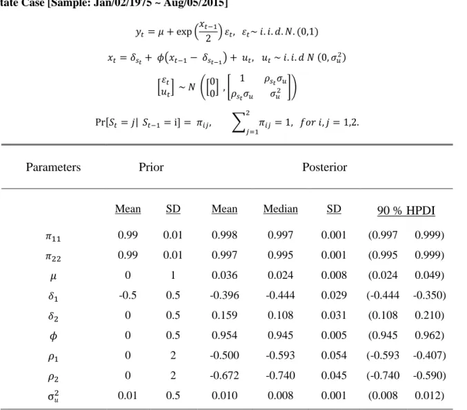
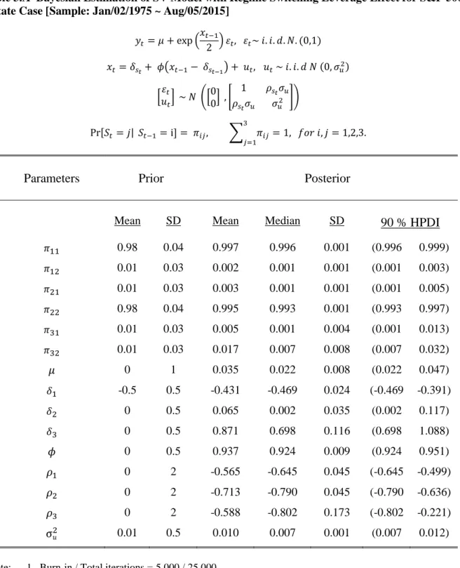
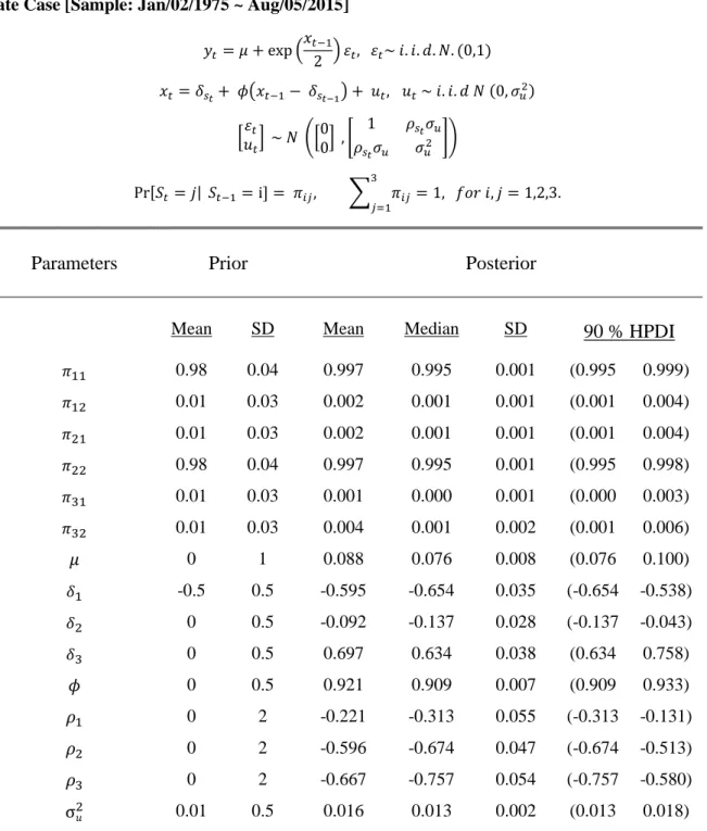
Another goal of this paper is to properly investigate the relationship between volatility and return in the U.S. stock markets in the presence of regime switching by employing the econometric tool developed. Black (1976) and Christie (1982) found empirical evidence that volatility tends to rise in response to bad news on returns but falls in response to good news on returns. This phenomenon is usually explained by the financial leverage effect7_{. Omori et al. (2007) empirically showed that the leverage effect is an important feature} of the U.S. stock market by using stochastic volatility models with leverage. In the stochastic volatility literature, the leverage effect is often assumed to be constant, including as described in Omori et al. (2007). Following Bandi and Renò (2012), I allow for a regime-dependent leverage effect in the context of a discrete time stochastic volatility model. In the proposed stochastic volatility model, the correlation parameter that captures the leverage effect is specified by a function of the regime specific means of log volatility and regime changes that are endogenously estimated within a Bayesian framework. Bandi and Renò (2012), in contrast, arbitrarily chose some deterministic threshold values of the spot volatility to distinguish different regimes in their parametric models. The empirical model is applied to daily S&P 500 and NASDAQ returns from the first week of January 1975 to the first week of August 2015. The Bayesian posterior means of the correlation parameters turn out to be significantly different across high- and low-volatility regimes. In particular, the Bayesian estimates indicate that the stronger (weaker) leverage effect is associated with a high (low)-volatility regime. Based on the Deviance Information Criterion (DIC) by Spiegelhalter et al. (2002), it is shown that the models with the regime-dependent leverage effect are always preferred to those with the constant leverage effect, regardless of the number of regimes. This empirical result confirms the time-varying leverage effect in the U.S. stock market described by Bandi and Renò (2012) within the parametric stochastic volatility models.

(7)

The rest of the paper is organized as follows. In Section 2, I introduce model specification and derive modified sequential Monte Carlo and backward simulation algorithms for a general NLG-SSSM. Section 3 provides details of the proposed PG sampler and illustrates its performance using a simulation study. In Section 4, I demonstrate the proposed technique on data from the U.S. stock market. Concluding remarks are provided in Section 5.

2 Model Specification and Particle Filtering-Smoothing

Non-linear/non-Gaussian Switching State-Space Models (NLG-SSSM) are a class of models in which the structure and the parameters of a non-linear state-space model switch according to discrete latent processes8_. A state space model consists of the measurement equationF(.) and the transition equationH(.):

yt=Fs0:t(x0:t, t) (1)

xt=Hs0:t(x0:t−1, ut)

where the dynamic system is observed over a time intervalt = 1,2, ..., T;xt ∈ X is the unobserved state vector; Yt∈Y is the observation vector; x0:t={x0, x1, ..., xt}, ands0:t={s0, s1, ..., st}; andut andt are identically distributed random variables with zero means and are not serially correlated9_{. The properties of} the state space model such as dimensions, functional forms, and model parameters shift over time according to a set of discrete latent variables s0:t = {s0, s1, ..., st}. The NLG-SSSM is parameterized by unknown parametersβst, subject to the discrete latent variablest. The latent variablestfollows a K-state first-order

Markov switching process with the following transition probabilities:

p(st=j|st−1=k) =πkj, K

X

j=1

πkj= 1, i, k= 1,2, ..., K. (2) The model parameters under K-regimes and the transition probabilities are denoted byθ={β1, β2, ..., βK, π} ∈ Θ. The hierarchical structure of the non-linear/non-Gaussian SSSM specified by equations (1) and (2) is the main difference from that of a conventional non-linear/non-Gaussian state-space model with discrete states. The distributions of the initial states are associated with the prior densities gθ(x0, s0) = gθ(x0|s0)gθ(s0). The above NLG-SSSM does not possess the Markovian property. Although the measurement and transition equations often depend on just a few latent states in practice, I adhere to the general model specification throughout this paper for generality of exposition.

8_{The class of Switching State-Space Models is also referred to as Jump Markov Systems in the literature.}

9_{The functions}_F₍_._{) and}_H₍_._{) can contain additional exogenous variables, but potential exogenous variables are omitted for}

(8)

Our primary concern is to perform Bayesian inference in an NLG-SSSM. The two sets of latent variables

x0:T = {x0, x1, ..., xT}, s0:T = {s0, s1, ..., sT} and the model parameters θ are treated as unknowns and jointly estimated based on the posterior density given as:

p(θ, x0:T, s0:T|Y1:T)∝ T Y t=1 fθ(yt|x0:t, s0:t)gθ(xt|x0:t−1, s0:t)gθ(st|st−1) gθ(x0|s0)gθ(s0)π(θ) (3) wherefθ(.) andgθ(.) denote probability densities associated with equations (1) and (2), givenθ; π(θ) is the prior density ofθ. Because the posterior is not available in closed form, Bayesian inference is often infeasible without simulation-based methods.

2.1 Particle Filtering for a Non-linear/Non-Gaussian SSSM

To develop an efficient PMCMC algorithm, it is crucial to sample from the joint smoothing density of the latent state variables pθ(x0:T, s0:T|y1:T), where y1:T = {y1, y2, ..., yT}. To obtain the joint smoothing density, consider the following decomposition of the joint filtering densitypθ(x0:t, s0:t|y1:t):

Equation (4) shows that the joint filtering density can be defined recursively. Except for a few cases such as linear/Gaussian state space models, the exact joint filtering density cannot be obtained because

pθ(x0:t−1, s0:t−1|y1:t−1) andfθ(yt|y1:t−1) are not analytically tractable.

A sequential importance sampling (SIS) algorithm is developed to recursively approximatepθ(x0:t, s0:t|y1:t) using random samples called ‘particles’. A set of particles is denoted by{X0:t, S0:t}={x

(i) 0:t, s

(i)

0:t}Ni=1, in which

N represents the total number of particles. The N particles are generated from the following importance distribution in an SIS algorithm:

q(x0:t, s0:t) =q(xt|x0:t−1, s0:t)q(st|x0:t−1, s0:t−1)q(x0:t−1, s0:t−1) (5) where q(.)’s denote importance densities possibly depending upon the observation sequence y1:t. Usu-ally, q(x0:t−1, s0:t−1) is numerically approximated by a Dirac measure δ_{_x(i)

0:t−1,s (i)

0:t−1}(x0:t−1, s0:t−1) in a SIS algorithm. The Dirac measure places a unit probability mass on each path in {X0:t−1, S0:t−1} =

{x(_0:i)t−1, s (i)

0:t−1}Ni=1 that has been already generated up to time t−1. New states {Xt, St} ={x( i) t , s

(i) t }Ni=1 are sequentially generated from q(st|x0:t−1, s0:t−1) and q(xt|x0:t−1, s0:t) conditional on the corresponding

(9)

past sequence {X0:t−1, S0:t−1}={x(0:i)t−1, s (i)

0:t−1}Ni=1. By combining the new particles at timet with the old particle trajectories at time t−1, we obtain a new set of particle paths {X_0:(i)_t, S(_0:i)_t} = {x(_0:i)_t, s(_0:i)_t}N

i=1. A candidate distribution to generate new particles at timet is called an incremental importance distribution.

In practice, the incremental importance distributionsq(xt|x0:t−1, s0:t) andq(st|x0:t−1, s0:t−1) in equation (5) should be well designed to closely approximate the target joint filtering distribution. The simplest approach is to exploit the transition densities associated with equations (1) and (2) and ignore information in the observation sequence y1:t:

q(xt|x0:t−1, s0:t) =gθ(xt|x0:t−1, s0:t),

q(st|x0:t−1, s0:t−1) =gθ(st|st−1).

(6)

In the Appendix, the optimal incremental importance distributions are derived, including all relevant infor-mation to obtain the closest approxiinfor-mation to the target distribution. The optimal incremental importance distributions can be constructed using a modified unscented Kalman filter10_{(UKF) by Andrieu et al. (2003).} However, I confirm via a simulation that the computational costs of sampling from the optimal importance distributions far exceed its benefits, especially when combined with a PMCMC sampler. Therefore, the incremental importance distributions in equation (6) are employed in forward filtering for all simulations and applications throughout this paper.

As an importance distribution is usually not identical to the target distribution, we need to correct the corresponding approximations by imposing the following importance weights to generated particles:

10_{As pointed out by many authors, linear/Gaussian approximation to a general non-linear/non-Gaussian state-space model}

through UKF is not accurate when the non-linearity is severe. The approximation errors by UKF quickly accumulate as the sample size increases. Wan and van der Merwe (2001) therefore suggested using UKF to design the importance distribution of a particle filter. They also empirically show that the resulting particle filtering algorithm performs well in capturing unobserved states and estimating model parameters.

(10)

Because the importance weightω(ti)is only proportional to ¯ω (i) t ω

(i)

t−1due to the unknown normalizing constant

pθ(yt|y1:t−1), ¯ωt(i)ω (i) t−1 is self-normalized as: ˆ ω(ti)= ¯ ωt(i)ω (i) t−1 PN j=1ω¯ (j) t ω (j) t−1

which yields our estimate of the importance weight at time t. Additionally, note that the normalizing constant can be approximated by:

ˆ pθ(yt|yt−1) = N X i=1 ¯ ωt(i)ω (i) t−1.

A critical problem of the SIS algorithm is weight degeneracy11_{. Gordon et al. (1993) originally developed a} standard particle filter to solve weight degeneracy by including a resampling step in whichN random particles

{x˜(_0:i)t,s˜ (i)

0:t}Ni=1are re-drawn from the existing particles{x (i) 0:t, s

(i)

0:t}Ni=1according to the normalized importance weight {ωˆ(ti)}Ni=1. The additional resampling step replicates particles with high importance weights while removing particles with low importance weights to prevent weight degeneracy. It is worth mentioning that the standard particle filter described by Gordon et al. (1993) can be considered a special case of the auxiliary particle filter of Pitt and Shephard (1999)12_{. These particle filters are also known as sequential Monte Carlo} (SMC) methods. Because the resampling step allows us to obtain equally weighted particles approximately distributed from pθ(x0:t, s0:t|y1:t), a new set of weights {ω˜

(i) t = N1}

N

i=1 is assigned to resampled particles

{x˜(_0:i)_t,s˜(_0:i)_t}N

i=1. The joint smoothing density pθ(x0:T, s0:T|y1:T) of interest can be obtained by the recursive structure in equations (4) and (5) ast=T. In what follows, I provide a summary of an SMC algorithm for NLG-SSSM.

Algorithm 1-1: Sequential Monte Carlo (SMC)

i) Draw{s(0i)}iN=1 fromq(s0) and draw{x (i)

0 }Ni=1fromq(x0|s (i)

0 ). Save the normalized importance weights

{ωˆ0(i)= ¯ ω(₀i) PN j=1ω¯ (i) 0 }N i=1 where ¯ω (i) 0 = pθ(x(0i)|s (i) 0 )pθ(s(0i)) q(x(₀i)|s₀(i))q(s(₀i)) .

• Iterate step ii), iii), and vi) fort= 1,2, ..., T. ii) ResampleN particles{x˜(_0:i)_t₋₁,s˜(_0:i)_t₋₁}N

i=1from{x (i) 0:t−1, s (i) 0:t−1}Ni=1with probability{ωˆ (i) t−1}Ni=1and assign new importance weights{ω˜(_t₋i)₁= _N1}N

i=1. Rename the particles{x˜ (i) 0:t−1,˜s (i) 0:t−1}Ni=1into{x (i) 0:t−1, s (i) 0:t−1}Ni=1 and the importance weights{ω˜t(−i)1}Ni=1 into{ω

(i) t−1}Ni=1.

11_{Weight degeneracy is a phenomenon that most of the particles}_{_x(i) 0:t, s

(i) 0:t}

N

i₌₁diverge from their true latent states over time,

increasing the variance of importance weights, and eventually, all but one of the importance weights converge to zero.

12_{The auxiliary particle filter uses updated importance weights with information on}_y

t+1in resamplingxtandst. However,

this article does not explicitly attempt to implement the auxiliary particle filter due to high computational costs of estimating NLG-SSSM.

(11)

iii) Draw{s(ti)}Ni=1 from g(s (i) t |x (i) 0:t−1, s (i) 0:t−1) and draw{x (i) t }Ni=1 from g(x (i) t |x (i) 0:t−1, s (i) 0:t). Set {x (i) 0:t} N i=1= {x(_0:i)_t₋₁, xt(i)}Ni=1and{s (i) 0:t} N i=1={s (i) 0:t−1, s (i) t }Ni=1. vi) Calculate the unnormalized weights: ¯ω(ti)ωˆ

¯ ω(_ti)ωˆ(_ti) −1 PN j=1ω¯ (i) t ωˆ (i) t−1 .

In the proposed SMC method, the importance sampling is repeatedly operated at each time period to generate various particle realizations {x(_0:i)_T, s(_0:i)_T}N

i=1 from pθ(x0:T, s0,T|y1:T). The target joint smoothing distribution is approximated by:

pθ(x0:T, s0,T|y1:T)≈ N X i=1 ˆ ω(_Ti)δ_{_x(i) 0:T,s (i) 0:T}( x0:T, s0:T) whereδ_{_x(i) 0:T,s (i) 0:T}(

x0:T, s0:T) places a unit probability mass on each path of{x( i) 0:T, s (i) 0:T} N i=1. Accordingly, we drawM particle trajectories from{x(_0:i)_T, s(_0:i)_T}N

i=1 with the normalized weight{ωˆ (i) T }

N

i=1to simulate from the joint smoothing distributionpθ(x0:T, s0,T|y1:T).

Algorithm 1-2: Forward Filtering forpθ(x0:T, s0:T|y1:T)

• Run Algorithm 1-1(SMC algorithm)and save the particle set {x_0:(i)_T, s(_0:i)_T}N

i=1 along with the nor-malized importance weights{ωˆ(_Ti)}N

i=1 at timeT. i) Draw{x˜(_0:j_T),s˜(_0:j_T)}M j=1 from{x (i) 0:T, s (i) 0:T} N

i=1 according to the normalized importance weights{ωˆ (i) T }

N i=1.

2.2 Backward Smoothing for a Non-linear/Non-Gaussian SSSM

The approximate joint smoothing distribution obtained using an SMC algorithm is often unreliable due to path degeneracy. For instance, when re-samplingxt andst in the SMC method, we discard many past trajectories in{x(_0:i)t, s

(i)

0:t}Ni=1, decreasing the number of unique particles at each time period. Consequently, the resulting particles{x(0:i)t, s

(i) 0:t}

N

i=1 share just a few common ancestors astincreases. This inevitably leads to a poor approximation of the joint smoothing distribution pθ(x0:T, s0:T|y1:T). As regimes change more frequently or the number of regimes is large, the path degeneracy problem gets worse, as shown by Andrieu et al. (2003) and Driessen and Boers (2005). Even if an increase in the number of particles can mitigate path degeneracy, huge computation costs are required for a PMCMC algorithm.

Based on the ideas of Godsill et al.(2004), we can effectively address the problem of path degeneracy by complementing forward filtering with additional backward smoothing for NLG-SSSM. Consider the following

(12)

where pθ(xt+1:T, st+1:T|xt, st) = [QTτ=tgθ(xτ|xt:τ−1, st:τ)]gθ(st+1|st) due to the hierarchical structure of NLG-SSSM.

As shown in equation (9), the smoothing recursion requires the joint marginal filtering densitypθ(xt, st|y1:t). The SMC algorithm introduced in the previous section can provide a numerical approximation ofpθ(xt, st|y1:t) as a direct application. The joint marginal densitypθ(xt, st|y1:t) is given by:

pθ(x0:t, s0:t|y1:t) =

X

s0:t−1

Z

pθ(x0:t, s0:t|y1:t)dx0:t−1.

In practice, integrating over the all the past states can be easily done by simply discarding{x(_0:i)t−1, s (i) 0:t−1}Ni=1 up to timet−1 and keeping only{x_t(i), s(_ti)}N

i=1at timetwith the normalized importance weights{ωˆ (i) t }

N i=1. The saved particles and importance weights approximate the joint marginal densitypθ(xt, st|y1:t):

pθ(xt, st|y1:t)≈ N X i=1 ˆ ω(ti)δ_{_x(i) t ,s (i) t }( xt, st) whereδ_{_x(i) t ,s (i) t }(

xt, st) is the Dirac measure and ˆω (i)

t is the normalized weight attached to particlesx (i) t and

s(ti).

Particles at timetare updated conditional onxt+1:T andst+1:T according to equation (9) using additional importance sampling and resampling steps as follows:

pθ(xt, st|xt+1:T, st+1:T, y1:T)≈ N X i=1 ˆ ω_t(i_|_T)δ_{_x(i) t ,s (i) t }(xt, st). (10)

(13)

where pθ(xt+1:T, st+1:T|xt, st) = [QT_τ₌_tgθ(xτ|xt:τ−1, st:τ)]gθ(st+1|st). The empirical distribution in equa-tion (10) is employed to generate particles {x˜(ti),s˜

(i)

t }Mi=1 sequentially backward in time conditional on

{x(ti+1:) T, s (i)

t+1:T}Mi=1andy1:T. The following is the summary of the backward simulation for NLG-SSSM.

Algorithm 1-3: Backward Smoothing for pθ(x0:T, s0:T|y1:T)

• RunAlgorithm 1-1 (SMC algorithm)and save the particle set{x(ti), s (i)

t }Ni=1 along with the normal-ized importance weights {ωˆ(_ti)}N

i=1 fort= 1,2, ..., T. i) Draw{x˜T,˜sT}from {x (i) T , s (i) T } N

i=1 with the normalized importance weights{ωˆ (i) T }

N i=1.

• Iterate step ii), and iii) fort=T −1, T−2, ..,0

ii) Calculate the modified normalized weights ˆω_t(i_|_T) conditional on ˜xt+1:T and ˜st+1:T. iii) Draw ˜xt,s˜tfrom{x(ti), s

(i)

t }Ni=1according to the modified importance weight{ωˆ (i) t|T}

N i=1.

• Repeat step i),ii), and iii) M times and save {x˜(_0:i)_T,s˜(_0:i)_T}M i=1.

The backward smoothing algorithm can be operated to generate various particle realizations{x˜(_0:i)_T,˜s(_0:i)_T}M i=1 from the joint smoothing distribution pθ(x0:T, s0,T|y1:T). As briefly discussed in the previous section, the forward filtering algorithm to approximatepθ(x0:T, s0,T|y1:T) seriously suffers from path degeneracy. The backward smoothing algorithm, however, is free from path degeneracy because it exploits al ofl the generated particles at each time, going backward in time. This superior feature of the backward smoothing algorithm is the key to successfully developing an efficient PG sampler in the next section.

3 Particle Markov Chain Monte Carlo Methods for a

non-linear/non-Gaussian SSSM

To simulate the posterior distributionp(θ, x0:T, s0:T|y1:T), one may attempt to alternatively sampleθfrom

p(θ|x0:T, s0:T, y1:T),x0:T fromp(x0:T|s0:T, θ, y1:T) ands0:T fromp(s0:T|θ, x0:T, y1:T). While this conventional Gibbs sampling approach seems straightforward to implement, there are some practical problems due to the presence of the regime indicator variable.

First, a multi-move sampler is not available for drawing s0:T from p(s0:T|θ, x0:T, y1:T) when the path dependence problem is encountered in the transition and measurement equations. Note that the current

(14)

observation and the continuous state in equation (1) are dependent on the entire sequence of the regime indicator variable up to time t. As the regime indicator variables are unobservable, we need to integrate over all possible regime paths when computing the likelihood, which is essential for a multi-move sampler. However, as the number of possible cases increases exponentially with t, evaluating the likelihood is not feasible in this case. A single-move sampler provides another option. However, as shown in Liu et al. (1994), Scott (2002), and Kim and Kim (2015), it is hard to obtain a correct stationary distribution via a single-move sampler if the regime indicator variable is very persistent or has absorbing states. In Section 2.4, it will be shown that the proposed PG sampler in this article produces reliable Bayesian estimates and achieves fast mixing even for an NLG-SSSM with the path dependence feature.

Second, the MCMC transition kernel becomes degenerate when the continuous state and the discrete regime indicator variables are perfectly correlated. A prominent example is provided by the Bayesian change-point models in Pesaran et al. (2006) and Koop and Potter (2007). Asx0:T is generated in a block conditional ons0:T andy1:T and thens0:T is generated conditional onx0:T andy1:T, this sampling scheme is degenerate. This is becausextdoes not change ifst= 0; conversely, ifxtis constant, then stis generated to be 0.

All these practical problems are solved by draw x0:T and s0:T from the joint smoothing distribution

p(x0:T, s0:T|y1:T, θ) using Gibbs sampling methods. The main difficulties in deriving a proper Gibbs sampler are that the joint smoothing distribution shows complex patterns of dependence among the latent variables, and sampling{x0:T, s0:T}directly from the joint smoothing distributionp(x0:T, s0:T|y1:T, θ) is not possible in general as a result of non-linearity and non-Gaussianity. I adopt a PG sampling approach to estimate NLG-SSSM following Andrieu et al. (2010) and illustrate that the proposed PG sampler performs well in various cases. Like any other Gibbs samplers, the PG sampling method does not require additional accept/reject steps, which produce mixing properties that are better than those of particle Metropolis-Hastings samplers. For a valid particle approximation to a Gibbs sampler, I use an artificial target distribution Ψ(.) that incorporates all of the randomness generated by an SMC method. If the new extended target distribution Ψ(.) admits the original posteriorp(θ, x0:T, s0:T|y1:T) as a marginal, a valid Gibbs sampler can be designed by Ψ(.). For this purpose, the particle Gibbs sampler is augmented by auxiliary variables to capture the additional randomness of an SMC method:

At={a( i) t }

N i=1.

The so-called ancestor index a(ti) ∈ {1,2, ..., N} is the index variable of the ancestor at timet−1 of i-th particles{x(ti), s (i) t }. For example, ifx (5) t−1and s (5)

t−1 are drawn forx (i) t ands

(i)

t in the resampling step of an SMC method, the index variable yieldsa(ti) = 5. Using the ancestor index, entire particle trajectories are

(15)

constructed by tracing back to their ancestral lineages recursively: x(_0:i)_t={x(a (i) t ) 0:t−1, x (i) t }, s (i) 0:t={s (a(_ti)) 0:t−1, s (i) t }for i= 1,2, ..., N.

Now, let K ∈ {1,2, ..., N}be the index of a fixed reference trajectory. We can keep track of its ancestral lineage as follows: x(_0:K_T)={x(a (K) T ) 0:T−1, x (K) T }={x (a(a (K) T ) T−1 ) 0:T−2 , x (a(_TK)) T−1 , x (K) T }=... s(_0:K_T)={s(a (K) T ) 0:T−1, s (K) T }={s (a(a (K) T ) T−1 ) 0:T−2 , s (a(_TK)) T−1 , s (K) T }=...

For the fixed reference trajectory, an additional indexbtis used for notational simplicity. The index for the reference trajectory is defined as:

x(_0:K_T)=x(b0:T) 0:T ={x (b0) 0 , x (b1) 1 , ..., x (bT−1) T−1 , x (bT) T } s(_0:K_T)=s(b0:T) 0:T ={s (b0) 0 , s (b1) 1 , ..., s (bT−1) T−1 , s (bT) T }

According to the definition ofbt, we can rewrite the indexbtin terms of the ancestor index asbt=K for

t=T andbt=at(b+1t+1)fort= 0, ..., T−1. The introduced indices are auxiliary variables in an SMC sampler and will play a key role later in deriving valid MCMC transition kernels. Finally, the remaining latent states except the reference trajectory are denoted byX(−b0:T)

0:T andS (−b0:T)

0:T .

Using the ancestor index variables, the density of the SMC in Section 2.1 is defined as: Φ(X0:T, S0:T, A1:T|θ) = N Y i=1 q(x(₀i)|s₀(i))q(s(₀i)) T Y t=1 N Y i=1 ¯ ω_t(i₋)₁ P jω¯ (j) t−1 q(x(ti)|x (a(_ti)) 0:t−1, s (i) 0:t)q(s (i) t |x (a(_ti)) 0:t−1, s (a(_ti)) 0:t−1) = N Y i=1 q(x(₀i)|s₀(i))q(s(₀i)) T Y t=1 N Y i=1 Mtθ(a (i) t , x (i) t , s (i) t ) (12) in whichMθ t(a (i) t , x (i) t , s (i) t ) is given as follows: Mθ t(a (i) t , x (i) t , s (i) t ) = ¯ ω(_ti₋)₁ P jω¯ (j) t−1 q(x(ti)|x (a(_ti)) 0:t−1, s (i) 0:t)q(s (i) t |x (a(_ti)) 0:t−1, s (a(_ti)) 0:t−1), and X0:T = {x (i) 0:T} N i=1; S0:T = {s (i) 0:T} N i=1; A1:T = {a (i) 1:T} N

i=1; q(.) denote importance densities that may depend on the observation sequence y1:t. The unnormalized importance weights in equation (12) are given as follows: ¯ ωt(i)= fθ(yt|x( i) 0:t, s (i) 0:t)pθ(x( i) t |x (i) 0:t−1, s (i) 0:t)pθ(s( i) t |s (i) t−1) q(x(ti)|x (i) 0:t−1, s (i) 0:t)q(s (i) t |x (i) 0:t−1, s (i) 0:t−1) .

(16)

I note that the normalized importance weight ˆωt(i)= ¯ ω(_ti)ωˆ(_ti) −1 P jω¯ (j) t ωˆ (j) t−1 can be rewritten as ˆωt(i)= ¯ ω(_ti) P jω¯ (j) t because we assign _N1 to ˆω(t−i)1after resampling. Similarly, we can easily determine the conditional density of the SMC given a reference trajectoryx(b0:T)

0:T ands (b0:T) 0:T : Φ(X(−b0:T) 0:T ,S (−b0:T) 0:T , A (−b1:T) 1:T |θ, x (b0:T) 0:T , s (b0:T) 0:T , b0:T) = Φ(X0:T, S0:T, A1:T|θ) q(x(₀b0)|s₀(b0))q(s(₀b0))QT t=1 ¯ ω(_tbt) −1 P jω¯ (j) t−1 q(x(bt) t |x (b0:t−1) 0:t−1 , s (b0:t) 0:t )q(s (bt) t |x (b0:t−1) 0:t−1 , s (b0:t−1) 0:t−1 ) = N Y i=1 i6=b0 q(x(₀i)|s₀(i))q(s(₀i))× T Y t=1 N Y i=1 i6=bt Mtθ(a (i) t , x (i) t , s (i) t ) (13)

The extended target distribution to construct valid MCMC kernels is given by: Φ(θ, X0:T, S0:T, A1:T, K)≡Φ(θ, x( b0:T) 0:T , s (b0:T) 0:T , b0:T)Φ(X(− b0:T) 0:T , S (−b0:T) 0:T , A (−b0:T) 1:T |θ, x (b0:T) 0:T , s (b0:T) 0:T , b0:T) ≡ 1 NT+1p(θ, x (b0:T) 0:T , s (b0:T) 0:T |y1:T) × N Y i=1 i6=b0 q(x(₀i)|s₀(i))q(s(₀i))× T Y t=1 N Y i=1 i6=b0 Mtθ(a (i) t , x (i) t , s (i) t ) (14) where X0:T = {x( b0:T) 0:T , X (−b0:T) 0:T }; S0:T = {s( b0:T) 0:T , S (−b0:T)

0:T }; K ∈ {1,2, ..., N} is the index of a reference trajectory. A particle Gibbs sampler will be developed in this section to estimate NLG-SSSM by targeting the extended target distribution. The suggested sampling scheme will havep(θ, x0:T, s0:T|y1:T) as the stationary distribution by marginalizing over all the auxiliary variables by an SMC algorithm, as shown in Andrieu et al. (2010).

3.1 Benchmark Particle Gibbs

We are interested in sampling from p(θ, x0:T, s0:T|y1:T) based on a Particle Gibbs (PG) sampler. The main difficulty of the Bayesian inference is that the target density has a high-dimensional parameter space Θ×X(T+1)_×_S(T+1)_{. This problem can be alleviated by building a multi-stage Gibbs sampler including the} auxiliary variables as suggested by Andrieu et al. (2010). In what follows, I provide details of the benchmark PG sampler to estimate NLG-SSSM.

The first step of the benchmark PG sampler is to sample the index Kof a reference trajectory. This is exactly the same as drawing one particle trajectory from all generated particle trajectories using an SMC

(17)

method. The conditional distribution for the indexK is given by: Φ(K|θ, X0:T, S0:T, A1:T) = ¯ wT(K) PN j=1w¯ (j) T (15) based on the followingProposition 1.

Proposition 1 The conditionalΦ(K|θ, X0:T, S0:T, A1:T)under the extended targetΦ(θ, X0:T, S0:T, A1:T, K)

is proportional to the importance weight atT:

Φ(K|θ, X0:T, S0:T, A1:T)∝w¯ (K) T .

The proof ofProposition 1is given in the Appendix. Based onProposition 1, it is straightforward to sample a reference index Kfrom its conditional in equation (15).

In the second step of the standard PG sampler, we sampleθ based on a partially collapsed Gibbs step, which means that some of the random variables are marginalized before conditioning. It does not violate the invariance of the corresponding sampler. For more details, see van Dyk and Park (2008). From constructing he extended target distribution, the conditional distribution forθ is given by:

Φ(θ|x(b0:T) 0:T , s (b0:T) 0:T , b0:T) =p(θ|x(_0:b0:TT), s (b0:T) 0:T , y1:T) (16) Note that in practice, sampling θ from p(θ|x0:T, s0:T, y1:T) is much simpler than sampling θ conditional only on the observations y1:T13. I assume that samplingθ from its conditional distribution under Φ(.) is straightforward by either using conjugate priors or Metropolis-Hastings givenx(b0:T)

0:T , s (b0:T)

0:T .

The conditional distribution for the third step of the benchmark PG sampler is given in equation (13). More specifically, we generateN−1 particle trajectories conditional onθand a reference trajectory from the conditional distribution Φ(X(−b0:T) 0:T , S (−b0:T) 0:T , A (−b1:T) 1:T |θ, x (b0:T) 0:T , s (b0:T)

0:T , b0:T). To achieve this goal, we employ a so-called conditional SMC algorithm. Simply speaking, the conditional SMC method is an algorithm that generatesN−1 particles with the reference trajectory{x(b0:T)

0:T , s (b0:T)

0:T }fixed throughout the sampling process. Before introducing the conditional SMC sampler, it is worth mentioning that the actual values of the indices

b0:T are not important et all, and therefore, we can assign an alternative sequence tob0:T ={N, N, ..., N} as a matter of convenience. This is because the index sequence b0:T is just a convenient tool to keep track of the past latent variables in entire particle sets. The following algorithm is the conditional SMC method used in the benchmark PG sampler.

13_{For instance, the transition probabilities for}_s

t can be easily generated from the beta distributions when using conjugate

priors. When non-conjugate priors are used or conditional posteriors do not belong to well-known distributions for some parameters, we can employ Metropolis-Hastings algorithms within a Particle Gibbs sampling approach conditional on the latent states.

(18)

Algorithm 2-1: Conditional Sequential Monte Carlo (CSMC)

i) Draw {s(₀i)}Ni=1−1 from q(s0) and draw {x(0i)} N−1

i=1 from q(x0|s(0i)) sequentially. Set {x (N) 0 , s

(N) 0 } =

{x(₀b0), s(₀b0)}. Save the normalized importance weights{ωˆ(₀i)= ω¯ (i) 0 PN j=1ω¯ (i) 0 }N i=1where ¯ω (i) 0 = pθ(x(0i)|s (i) 0 )pθ(s(0i)) q(x(₀i)|s₀(i))q(s(₀i)) .

• Iterate step ii), iii), and vi) fort= 1,2, ..., T. ii) Draw ancestor indices{a(ti)}

N−1 i=1 with probability{ωˆ (i) t−1}Ni=1. Draw{s (i) t } N−1 i=1 fromg(s (i) t |x (a(_ti)) 0:t−1, s (a(_ti)) 0:t−1) and{x(ti)} N−1 i=1 fromg(x (i) t |x (a(_ti)) 0:t−1, s (a(_ti)) 0:t−1, s (i) t ) sequentially. iii) Seta(tN) = N and {x

(N) t , s (N) t } ={x (bt) t , s (bt)

t }. New trajectories are set by x (i) 0:t ={x (a(_ti)) 0:t−1, x (i) t } and s(_0:i)_t={s(a (i) t ) 0:t−1, s (i) t } fori= 1,2, ..., N. vi) Calculate the unnormalized weights: ¯ω(ti)=

¯ ω_t(i) PN j=1ω¯ (i) t fori= 1,2, ..., N.

Note that sampling ancestor indices {a(ti)} N−1

i=1 in step ii) is equivalent to resampling N −1 particles

{x˜(ti−)1,˜s (i) t−1} N−1 i=1 from {x (i) t−1, s (i) t−1}Ni=1with probability{ωˆ (i)

t−1}Ni=1. This completes the benchmark PG sam-pler for NLG-SSSM. The summary of the benchmark PG algorithm is given by the following.

Algorithm 2-2: Benchmark PG for Non-linear/non-Gaussian SSSM

Choose θ arbitrarily and draw {X0:T, S0:T, A1:T} by running Algorithm 1-1 (SMC algorithm):

{X0:T, S0:T, A1:T} ∼Φ(X0:T, S0:T, A1:T|θ)

• Iterate step i), step ii), and step iii) forr= 1,2, ..., R.

i) DrawK∈ {1,2, ..., N}(a reference trajectory) from: K∼Φ(K|θ, X0:T, S0:T, A1:T) And set {x(b0:T) 0:T , s (b0:T) 0:T }={x (K) 0:T, s (K) 0:T}. ii) Drawθ from: θ∼Φ(θ|x(b0:T)

0:T , s (b0:T) 0:T , b0:T) iii) Draw{X(−b0:T) 0:T , S (−b0:T) 0:T , A (−b1:T)

1:T } by runningAlgorithm 2-1(CSMC algorithm)from:

{X(−b0:T) 0:T , S (−b0:T) 0:T , A (−b1:T) 1:T } ∼Φ(X (−b0:T) 0:T , S (−b0:T) 0:T , A (−b1:T) 1:T |θ, x (b0:T) 0:T , s (b0:T) 0:T , b0:T) And set X0:T ={X(− b0:T) 0:T , x (b0:T) 0:T },S0:T ={S(− b0:T) 0:T , s (b0:T) 0:T },A1:T ={A(− b1:T) 1:T , b0:T−1}.

The variable K represents the index of a reference particle trajectory; R is the total number of MCMC iterations.

Many papers such as those by Whiteley (2010), Fredrik and Schon (2012), and Whiteley et al. (2011) recognize that a standard PG sampler seriously suffers from poor mixing due to path degeneracy. The same problem arises in the benchmark PG sampler when it is applied to NLG-SSSM. To address the issue of path degeneracy and poor mixing, I introduce an alternative PG sampler in the next section.

(19)

3.2 Proposed Particle Gibbs

An SCM algorithm with additional backward simulation substantially alleviates path degeneracy by shuffling particle trajectories backward in time. A PG sampler with ancestor sampling (PGAS) developed by Fredrik and Schon (2012) and Lindsten et al. (2014) implicitly incorporates the backward simulation by updating particle trajectories forward in time without adding explicit backward recursion. In this section, I propose a PGAS sampler for NLG-SSSM that targets the extended target distribution in equation (14) to resolve path degeneracy and improve mixing of the resulting MCMC chain.

The main difference between the proposed PG sampler and the benchmark PG sampler is in the treat-ment of the index variables b0:T−1 ={b0, b1, ..., bT−1} of a reference trajectory. While the benchmark PG sampler keeps a particular reference trajectory fixed at each MCMC iteration, the proposed PG sampler constructs a new particle trajectory by drawing the ancestor indices bt−1(= abtt) at each time. For in-stance, ifbt−1= 5 is drawn in a supplementary procedure, we accordingly set a new reference trajectory as

x(b0:t) 1:t ={x (b0:t−2) 1:t−2 , x (bt−1=5) t−1 , x (bt)

t }. This additional step to update the indicesb0:T−1 has a similar effect to that of backward recursion, which will be shown inProposition 2.

The first and second steps of the proposed PGAS sampler are exactly the same as those of the benchmark PG sampler. The index of a new reference trajectoryKis sampled among{X0:T, S0:T, A1:T}, which contains a previously accepted reference trajectory. Based onProposition1,K is drawn according to the importance weight ¯ω_T(i) at T. As before, we assume that sampling θ is straightforward based on the conditional in equation (16).

Using partially collapsed Gibbs steps and the extended target density in equation (14), we have the following conditional to generate particles given a reference trajectory fort= 0:

Φ(X₀(−b0), S₀(−b0)|θ, x(b0:T) 0:T , s (b0:T) 0:T , b0:T) = N Y i=1 i6=b0 q(x(₀i)|s₀(i))q(s(₀i)) (17) and, fort= 1,2, ..., T Φ(X(−bt) t ,S (−bt) t , A (−bt) t |θ, X0:t−1, S0:t−1, A1:t−1, x( bt:T) t:T , s (bt:T) t:T , bt−1:T) = Φ(X(−bt) t , S (−bt) t , A (−bt) t |θ, X (−b0:t−1) 0:t−1 , S (−b0:t−1) 0:t−1 , A (−b1:t−1) 1:t−1 , x (b0:T) 0:T , s (b0:T) 0:T , b0:T) = Φ(X (−b0:t) 0:t , S (−b0:t) 0:t , A (−b0:t) 0:t |θ, x (b0:T) 0:T , s (b0:T) 0:T , b0:T) Φ(X(−b0:t−1) 0:t−1 , S (−b0:t−1) 0:t−1 , A (−b0:t−1) 0:t−1 |θ, x (b0:T) 0:T , s (b0:T) 0:T , b0:T) = N Y i=1 i6=bt ¯ ωt(i−)1 P jω¯ (j) t−1 q(x(ti)|x (a(_ti)) 0:t−1, s (a(_ti)) 0:t−1, s (i) t )q(s (i) t |x (a(_ti)) 0:t−1, s (a(_ti)) 0:t−1) = N Y i=1 i6=bt Mtθ(a (i) t , x (i) t , s (i) t ) (18)

(20)

Equations (17) and (18) show that we can draw {X₀(−b0), S₀(−b0)} using q(x₀(i)|s(₀i))q(s(₀i)) and then draw {X(−b0:t) 0:t , S (−b0:t) 0:t , A (−b1:t)

1:t }from the combination of the resampling weight and the importance distributions, ¯ ω_t(i) −1 P jω¯ (j) t−1 q(x(ti)|x (a(_ti)) 0:t−1, s (a(_ti)) 0:t−1, s (i) t )q(s (i) t |x (a(_ti)) 0:t−1, s (a(_ti))

0:t−1). Lastly, the transition kernel to produce a new ancestor indexbt−1(=abtt) is given inProposition 2.

Proposition 2 The conditionalΦ(bt−1|θ, X0:t−1, S0:t−1, A0:t−1, x(tb:Tt:T), s (bt:T)

t:T , bt:T)under the extended target Φ(θ, X0:T, S0:T, A1:T, K) is proportional to the following backward kernel att−1:

Φ(bt−1|θ,X0:t−1, S0:t−1, A0:t−1, x(tb:Tt:T), s (bt:T) t:T , bt:T) ∝ T Y l=t fθ(yl|x( b0:l) 0:l , s (b0:l) 0:l )gθ(xl|x (b0:l−1) 0:l−1 , s (b0:l) 0:l )gθ(s( bl) l |s (bl−1) l−1 ) ˆ ω(bt−1) t−1

Thus, we drawbt−1(=at(bt))∈ {1,2, ..., N}with the following probability:

Appendix provides the proof ofProposition 2. I note, in a special case, that the backward kernel inProposition 2is equivalent to that of backward simulation in equation (9).

Lemma 1 For a Markov state space model, the conditionalΦ(bt−1|θ, X0:t−1, S0:t−1, A0:t−1, x( bt:T)

t:T , s (bt:T)

t:T , bt:T)

is proportional to the backward kernel used in backward simulation:

Φ(bt−1|θ,X0:t−1, S0:t−1, A0:t−1, x(tb:Tt:T), s (bt:T) t:T , bt:T) ∝fθ(yt|x (bt) t , s (bt) t )gθ(xt|x (bt−1) t−1 , s (bt) t )gθ(s (bt) t |s (bt−1) t−1 )ˆω (bt−1) t−1

The proof of Lemma 1 is straightforward using the special dependence structure of a Markov state space model; I therefore skip the proof for brevity. Based on the derived MCMC kernels, a modified conditional SMC with ancestor sampling is introduced, which is crucial for implementing the proposed PG sampler with ancestor sampling.

Algorithm 3-1: CSMC with Ancestor Sampling (CSMC-AS)

i) Draw {s(₀i)}Ni=1−1 from q(s0) and draw {x(0i)} N−1

i=1 from q(x0|s(0i)) sequentially. Set {x (N) 0 , s

(N) 0 } =

{x(₀b0), s(₀b0)}. Save the normalized importance weights{ωˆ(₀i)= ω¯ (i) 0 PN j=1ω¯ (i) 0 }N i=1where ¯ω (i) 0 = gθ(x(0i)|s (i) 0 )gθ(s(0i)) q(x(₀i)|s₀(i))q(s(₀i)) .

(21)

• Iterate step ii), iii), and vi) fort= 1,2, ..., T. ii) Draw ancestor indices{a(ti)}

N−1 i=1 according to probability{ωˆ (i) t−1}Ni=1. Draw{s (i) t } N−1 i=1 fromq(s (i) t |x (a(_ti)) 0:t−1, s (a(_ti)) 0:t−1) and{x(ti)} N−1 i=1 fromq(x (i) t |x (a(_ti)) 0:t−1, s (a(_ti)) 0:t−1, s (i) t ) sequentially. iii) Draw bt−1(= a(tbt)) with probability ˜ω

(i) t−1|T in equation (19). Set a (N) t = bt−1 and {x(tN), s (N) t } = {x(bt) t , s (bt)

t }. The trajectories are set byx (i) 0:t={x (a(_ti)) 0:t−1, x (i) t }ands (i) 0:t={s (a(_ti)) 0:t−1, s (i) t }fori= 1,2, ..., N. vi) Calculate the unnormalized weights ¯ω(ti)=

¯ ω_t(i) PN j=1ω¯ (i) t fori= 1,2, ..., N.

Note that sampling ancestor indices {a(ti)} N−1

i=1 in step ii) is equivalent to resampling N −1 particles

{x˜(_ti₋)₁,˜s_t(₋i)₁}Ni=1−1 from{x (i) t−1, s (i) t−1}Ni=1 with probability{ωˆ (i)

t−1}Ni=1, as before. The summary of the proposed PG with ancestor sampling to estimate NLG-SSSM is given below.

Algorithm 3-2: PGAS for a Non-linear/non-Gaussian SSSM

Chooseθ arbitrarily and draw{X0:T, S0:T, A1:T} by runningAlgorithm 1-1(SMC algorithm)from:

{X0:T, S0:T, A1:T} ∼Φ(X0:T, S0:T, A1:T|θ)

0:T , s (b0:T)

0:T , b0:T) iii) Draw{X₀(−b0), S₀(−b0)}and{bt−1(=a(tbt)), X

(−bt)

t , S (−bt)

t , A (−bt)

t }for t = 1,2,...,T by runningAlgorithm

3-1 (CSMC-AS algorithm). whereX0:t={x( b0:t) 0:t , X (−b0:t) 0:t };S0:t={s( b0:t) 0:t , S (−b0:t) 0:t };A1:t={A(− b1:t)

1:t , b0:t−1};Krepresents the index of a reference particle trajectory;Ris the total number of MCMC iterations. The proposed PGAS sampler allows a reference trajectory to change its ancestry as the conditional SMC with ancestor sampling is operated in the forward direction. This approach is more robust to path degeneracy and enables a faster-mixing MCMC kernel than the benchmark PG sampler.

Though the ancestor sampling technique helps avoid path degeneracy by shuffling the ancestor indices and reducing the correlation between the particle trajectories, it cannot be applied to an NLG-SSSM with a degenerate transition equation. In such a model, the only previous particle trajectory that contains a particular future particle is that from which the future particle was originally generated. Hence, the probability of updating previous particle trajectories in ancestor sampling is always zero at every time

(22)

period unless new values of the latent states are jointly generated along with the corresponding ancestor indices.

3.3 Proposed Particle Gibbs for a Degenerate Transition Equation

Building upon the idea of Lindsten et al. (2014), Carter et al. (2014) 14_{, and Bunch et al. (2015), I} incorporate particle rejuvenation to estimate degenerate NLG-SSSM. The main idea of the new algorithm is to generates new values of latent states {xt, st} along with ancestor indices bt−1(=a(

bt)

t ) of a reference trajectory at each MCMC iteration. In the proposed scheme, new values of the latent states are not restricted to the output of a SMC procedure and are also drawn with more relevant information than the conditional SMC method. More specifically, additional importance distributions are designed to approximate a properly chosen backward kernel to simultaneously sample an ancestor index and new values for the associated latent states{xt, st}. Unlike the PGAS sampler inAlgorithm 5-2, information on the future states{xt+1:T, st+1:T} is incorporated in drawing{xt, st}.

All of the MCMC steps are the same as those of Algorithm 5-2, except fir step iii). The following proposition provides a justification for using the backward kernel to jointly generate new values of the latent states and the ancestor index.

Proposition 3 The conditionalΦ(x(bt)

t , s (bt)

t , bt−1|θ, X0:t−1, S0:t−1, A0:t−1, x(tb:Tt:T), s (bt:T)

t:T , bt:T)under the

ex-tended targetΦ(θ, X0:T, S0:T, A1:T, K)is proportional to the backward kernel at t−1: Φ(x(bt) t , s (bt) t , bt−1|θ,X0:t−1, S0:t−1, A0:t−1, x (bt+1:T) t+1:T , s (bt+1:T) t+1:T , bt:T) ∝ T Y l=t fθ(yl|x( b0:l) 0:l , s (b0:l) 0:l )gθ(xl|x (b0:l−1) 0:l−1 , s (b0:l) 0:l )gθ(s (bl) l |s (bl−1) l−1 ) ˆ ω(bt−1) t−1

The proof ofProposition 3 is given in the Appendix, which is similar to the proof ofProposition 2. Analo-gously, it can be easily verified that the latent states of the initial period are sampled based on the following MCMC kernel. Φ(x(₀b0), s₀(b0)|θ,x(b1:T) 1:T , s (b1:T) 1:T , b0:T) ∝ T Y l=1 fθ(yl|x (b0:l) 0:l , s (b0:l) 0:l )gθ(xl|x (b0:l−1) 0:l−1 , s (b0:l) 0:l )gθ(s (bl) l |s (bl−1) l−1 ) gθ(x (b0) 0 |s (b0) 0 )gθ(s (b0) 0 ) We can also see that the backward kernel inProposition 3is simplified for a Markov state space model.

14_{Carter et al. (2014) developed PMCMC samplers with a strategy similar to the particle rejuvenation technique. However,}

they specified a different extended target distribution to implement their methods and thus modified conditional SMC methods. Following Bunch et al. (2015), I do not change the original extended target distribution.

(23)

Lemma 2 For a Markov state space model, the conditionalΦ(x(bt) t , s (bt) t , bt−1|θ, X0:t−1, S0:t−1, A0:t−1, x(tb:Tt:T), s (bt:T) t:T , bt:T)

under the extended targetΦ(θ, X0:T, S0:T, A1:T, K)is proportional to the backward kernel used in backward

simulation: Φ(x(bt) t ,s (bt) t , bt−1|θ, X0:t−1, S0:t−1, A0:t−1, x(tb:Tt:T), s (bt:T) t:T , bt:T) ∝gθ(x (bt+1) t+1 |x (bt) t , s (bt+1) t+1 )gθ(s (bt+1) t+1 |s (bt) t )fθ(yt|x (bt) t , s (bt) t )gθ(xt|x (bt−1) t−1 , s (bt) t )gθ(s (bt) t |s (bt−1) t−1 )ˆω (bt−1) t−1 I skip the derivation ofLemma 2 for brevity. The MCMC procedure associated with the above backward kernel involves partially collapsed Gibbs steps and leaves Φ(.) invariant, as before. While the backward kernel inProposition 2resembles that of Proposition 3, proper methods to implement those steps are quite different. The normalizing constant of the backward kernel in Proposition 2 is easily calculated based on equation (19) in that we sample only the ancestor indexbt−1of a reference trajectory. On the other hand, the normalizing constant of the backward kernel inProposition 3to jointly draw{xt, st, bt−1}is not analytically tractable in general.

We can handle this problem by constructing MCMC kernels, leaving the conditional distributions in

Proposition 3(fort = 0 and fort = 1,2, ..., T) invariant. For instance, a conditional importance sampling (CIS) technique can be applied to approximate the conditional distributions at each time period. Consider the following importance distribution:

W(xt, st, bt−1) = Ψ(xt, st|x∗( bt) t , s ∗(bt) t , x (bt−1) 0:t−1, s (bt−1) 0:t−1, x (bt+1:T) t+1:T , s (bt+1:T) t+1:T ) ν(bt−1) t−1 PN j ν (j) t−1 for t= 1,2, ..., T (20) where{x∗(bt) t , s ∗(bt)

t }are the previously accepted MCMC draws and{xt, st, bt−1}are newly generated draws. Similarly, the importance distribution fort= 0 andt=T is properly designed by modifying equation (20). The above importance distribution indicates that a new ancestor index bt−1 of a reference trajectory is first sampled from a proposal weightv(bt−1)

t−1 , and new values of the latent states{xt, st} are then generated conditional on the previously accepted{x∗(bt)

t , s

∗(bt)

t }, the new past reference trajectory{x (bt−1) 0:t−1, s

(bt−1) 0:t−1}up to timet−1 and all the future reference trajectory{x(bt+1:T)

t+1:T , s (bt+1:T)

t+1:T }. The summary is given below for the CIS algorithm in whichC denotes the total number of particles used.

Algorithm 4-1: Conditional Importance Sampling (CIS) at timet

i) Set{x(_tC), s_t(C)}={x(bt)

t , s (bt)

t }.

• Iterate step ii) and step iii) forc= 1,2, ..., C−1. ii) Draw ancestor indexb(tc−)1∈ {1,2, ..., N}with probability

ν(bt−1) t−1 PN j ν (j) t−1 . Setx(b (c) t−1) 0:t−1 ={x (b0:t−2) 0:t−2 , x (b(_tc) −1) t−1 } ,s (b(_tc) −1) 0:t−1 ={s (b0:t−2) 0:t−2 , s (b(_tc) −1) t−1 }.

(24)

iii) Draw{x(tc), x (c) t }from Ψ(xt, st|x( bt) t , s (bt) t , x (b(_tc) −1) 0:t−1, s (b(_tc) −1) 0:t−1, x (bt+1:T) t+1:T , s (bt+1:T) t+1:T ). Setx(_0:c_T) ={x(b (c) t−1) 0:t−1, x (c) t , x (bt+1:T) t+1:T } ands (c) 0:T ={s (b(_tc) −1) 0:t−1, s (c) t , s (bt+1:T) t+1:T }. vi) Calculate the unnormalized weights forc= 1,2, ..., C:

¯ τt(c)= QT l=tfθ(yl|x (c) 0:l, s (c) 0:l)pθ(xl|x (c) 0:l−1, s (c) 0:l)pθ(s (c) l |s (c) l−1) ˆ ω(b (c) t−1) t−1 Ψ(x(tc), s (c) t |x (bt) t , s (bt) t , x (b(_tc₋)₁) 0:t−1, s (b(_tc₋)₁) 0:t−1, x (bt+1:T) t+1:T , s (bt+1:T) t+1:T )ν (b(_tc₋)₁) t−1 Obtain the normalized weights: ˆτt(c)=

¯ τ_t(c) PC j=1¯τ (j) t . v) Draw: {xt, st, bt−1} from{x( c) t , s (c) t , b (c) t−1}Cc=1 with probability ˆτ (c) t .

We can perform conditional importance sampling with largeC to enhance the mixing property in exchange for increasing computational costs. Using the derivation by Andrieu et al. (2010), it can be shown that the CIS admits the target Markov kernel inProposition 3as a stationary distribution. Indeed, any valid MCMC kernel such as the Metropolis-Hastings kernel can be used to approximate the target kernel. As a proper importance distribution in the CIS is dependent on the structure of a state space model of interest, we will discuss this issue based on a particular SSSM in the next section.

Now, the details of step iii) of the proposed PG sampler with particle rejuvenation are introduced in the following algorithm with the CIS scheme.

Algorithm 4-2: CSMC with Particle Rejuvenation (CSMC-PR)

i) Draw{s(₀i)}Ni=1−1from theq(s0) and draw{x(0i)} N−1

i=1 from q(x0|s(0i)) sequentially.

ii) Draw{x(₀b0), s₀(b0)} from the Markov kernelW(.) in equation (20) and set {x₀(N), s₀(N)}={x₀(b0), s(₀b0)}. Save the normalized importance weights {ωˆ(₀i)= ω¯

(i) 0 PN j=1ω¯ (i) 0 }N i=1 where ¯ω (i) 0 = gθ(x (i) 0 |s (i) 0 )gθ(s (i) 0 ) q(x(₀i)|s₀(i))q(s(₀i)) .

• Iterate step iii), vi), and v) for t= 1,2, ..., T. iii) Draw ancestor indices{a(ti)}

N−1 i=1 with probability{ωˆ (i) t−1}Ni=1. Draw{s (i) t } N−1 i=1 fromq(s (i) t |x (a(ti)) 0:t−1, s (a(ti)) 0:t−1) and{x(ti)} N−1 i=1 fromq(x (i) t |x (a(ti)) 0:t−1, s (a(ti)) 0:t−1, s (i) t ) sequentially. iii) RunAlgorithm 4-1 (CIS algorithm)to draw{x(bt)

t , s (bt) t , bt−1}. Seta (N) t =bt−1and{x( N) t , s (N) t }= {x(bt) t , s (bt)

t }. New particle trajectories are set by x (i) 0:t = {x (a(_ti)) 0:t−1, x (i) t } and s (i) 0:t = {s (a(_ti)) 0:t−1, s (i) t } for i= 1,2, ..., N.

vi) Calculate the unnormalized weights: ¯ω(ti)=

¯ ω(_ti) PN j=1ω¯ (i) t fori= 1,2, ..., N.

(25)

The proposed algorithm is an extension of the PG algorithm by Lindsten et al. (2014) to estimate NLG-SSSM. The uniform ergodicity for the suggested algorithm can be demonstrated using the work of Lindsten et al. (2014). The summary of the proposed PG sampler for degenerate NLG-SSSM is provided below.

Algorithm 4-3: PGAS with Particle Rejuvenation for a Non-linear/non-Gaussian SSSM

Chooseθ arbitrarily and draw{X0:T, S0:T, A1:T} by runningAlgorithm 1-1(SMC algorithm)from:

{X0:T, S0:T, A1:T} ∼Φ(X0:T, S0:T, A1:T|θ)

0:T , s (b0:T)

0:T , b0:T) iii) Draw{X₀(−b0), S(₀−b0)} and{bt−1(=a(tbt)), x

(bt) t , s (bt) t },{X (−bt) t , S (−bt) t , A (−bt) t }for t = 1,2,...,T by

run-ning Algorithm 4-2(CSMC-PR algorithm).

whereX0:t={x (b0:t) 0:t , x (−b0:t) 0:t };S0:t={s (b0:t) 0:t , s (−b0:t) 0:t };A1:t={A (−b1:t)

1:t , b0:t−1};K represents the index of a reference particle trajectory; andRis the total number of MCMC iterations.

3.4 Implementation of Proposed Particle Gibbs

In practice, the extended target density in (14) and associated backwards kernels can be simplified ac-cording to the structure of a particular NLG-SSSM of interest. This section provides more details on how the suggested PG algorithms are implemented using two specific examples. First, consider the regime switching

stochastic volatility (SV) model by So et al. (1998): Example 1

yt=µ+exp( xt−1 2 )t, t∼N(0,1) (21) xt=δst+φ(xt−1−δst−1) +ut, ut∼N(0, σ 2 u)

whereytis the equity return at timet;xt−1is the latent log-volatility at timet; andE[tut] = 0. The current position ofxtis given by a function ofxt−1, st, andst−1 in the transition equation, and the observationyt is given by a nonlinear function ofxt−1 in the measurement equation. Becausext andyt depend only on a few past states in such a model structure, the backward kernel inProposition 2 reduces to:

(26)

Therefore, bt−1∈ {1,2, ..., N}is drawn with the normalized importance weight in (19).

Similarly, new values of the latent states and their ancestor indices are jointly simulated by step iii) of

Algorithm 4-3using the following MCMC kernel:

Before implementing the CIS procedure inAlgorithm 4-1, we should construct importance distributions that target the kernel in (23). First, the importance weight ¯τt(i)is simplified by usingν

(i) t−1= ˆω

(i)

t−1and the easily calculable likelihood functionfθ(yt|x(

bt−1)

t−1 ) in drawingbt−1. Thus, the ancestor indexbt(−c)1∈ {1,2, ..., N}of a reference trajectory is drawn with the updated ˆω(_ti₋)₁ as:

b(_tc₋)₁∼ fθ(yt|x (bt−1) t−1 )ˆω (bt−1) t−1 PN j=1fθ(yt|x (j) t−1)ˆω (j) t−1 .

New values of the latent states are efficiently generated using their transition densities:

s(tc)∼pθ(st|s (bt+1) t+1 , s (b(_tc) −1) t−1 ) = pθ(s (bt+1) t+1 |st)pθ(st|s (b(_tc) −1) t−1 ) P stpθ(s (bt+1) t+1 |st)pθ(st|s (b(_tc) −1) t−1 ) and x(_tc)∼pθ(xt|x (bt+1) t+1 , x (b(_tc) −1) t−1 s (bt+1) t+1 , s (c) t , s (b(_tc) −1) t−1 )∝pθ(x (bt+1) t+1 |xt, s (bt+1) t+1 , s (c) t )pθ(xt|x (b(_tc) −1) t−1 , s (c) t , s (b(_tc) −1) t−1 ) It is shown in Appendix that x(tc) followsN(µt, Vt) where Vt = σ

2

u

(1+φ2₎; µt=δst +

φ

(1+φ2₎((xt+1−δst+1) + (xt−1−δst−1)). The unnormalized importance weight ˆτ

(c)_{in the CIS algorithm therefore is given by:} ˆ τ(c)=fθ(yt+1|x(tc))[ X st pθ(s (bt+1) t+1 |st)pθ(st|s (b(_tc) −1) t−1 )]pθ(x (bt+1) t+1 |x (b(_tc) −1) t−1 s (bt+1) t+1 , s (c) t , s (b(_tc) −1) t−1 ).

After sampling necessary random samples, the most likely particle set and the corresponding ancestor index are accepted with the importance weight ˆτ(c)_.

Another example of a NLG-SSSM is given as follows: Example 2

y1,t=β0+β1ft+β2ft2+1,t t∼N(0, σ21)