The global implications of freer skilled migration.

T H E A U S T R A L I A N N A T I O N A L U N I V E R S I T Y

WORKING PAPERS IN ECONOMICS AND ECONOMETRICS

The global implications of freer skilled migration*

Rod Tyers, Iain Bain and Jahnvi Vedi College of Business and Economics

Australian National University

Working Papers in Economics and Econometrics No. 468 Australian National University

ISBN: 86831 468 4 August 2006

Corresponding author: Professor Rod Tyers School of Economics

College of Business and Economics Australian National University Canberra, ACT 0200

rod.tyers@anu.edu.au

*

participation behaviour, Terrie Walmsley for technical assistance with the GTAP Database and Dominique van der Mensbrugghe and Tim Hatton for useful discussions on the modelling of migration flows. Valuable comments were also offered at a World Bank seminar in July 2006, particularly by Alan Winters, Maurice Schiff and David Tarr.

The global implications of freer skilled migration

Abstract:

One consequence of the trade and technology driven increases in skill premia in the older industrial regions since the 1980s has been a perceived “skill shortage” in those regions, along with freer migration of skilled and professional workers from developing regions. While skilled migration flows remain too small to have large short-run effects on labour markets, a further opening to skilled migrants by the industrialised North could see substantial changes in labour markets and overall growth performance. The links between demographic change, migration flows and economic growth are here explored using a new demographic sub-model that is integrated with an adaptation of the GTAP-Dynamic global economic model in which regional households are disaggregated by age and gender. Skilled migration flows are assumed to be motivated by real wage differences to an extent that is variably constrained by immigration policies. A uniform relaxation of these constraints has most effect on labour markets in the traditional migrant destinations, Australia, Western Europe and North America, where it restrains the skill premium and substantially enhances GDP growth. Skill premia are raised, however, in regions of origin, and particularly in South Asia, although the extent of this is shown to depend sensitively on the responsiveness of skill acquisition to regional skill premia.

1. Introduction

Rising skill premia in industrial labour markets in the 1980s and 90s sparked a substantial literature on the effects of expanded trade with developing regions and the development and transmission of skill-using technological change.1 This literature offers clear evidence that skill demand has tended to outpace skill acquisition in these markets and that this is the primary cause of widening skill premia. At the same time, the older

industrialised regions have experienced declining fertility and, in Europe and Japan in particular, transitions to labour force decline.2 These trends have been enhanced by the extraordinary duration of the most recent period of sustained global economic expansion, the ageing of industrialised populations and the associated rise in demand for service skills and, for some regions, by the loss of skilled workers through emigration.3 Taken together, they have brought forth “skill shortages” in the older industrialised regions, along with policy changes that have begun to allow freer migration of skilled and professional workers from developing regions.4

1

See McDougall and Tyers (1997), Berman, Bound and Machin (1998) and Tyers et al. (1999).

2

See Bongaarts and Bulatao (2000), McDonald and Kippen (2001), Lee (2003).

3

The many reasons for skilled migration have received widespread attention in the migration literature. See, for example, Salt (1992, 1997) and Khoo et al. (2006). They are complicated by comparatively rapid fertility declines amongst educated families, from whence emerge the children with the greatest potential for skill-acquisition. Evidence for this is offered by d’Addio and d’Ercole (2005).

4

In Australia, skilled work visas have been made easier to obtain and applications for permanent residency by workers who enter on these visas, or who complete training in Australia, no longer require return to their home

While skilled migration flows remain too small to have large short-run effects on destination labour markets, a continued opening to skilled migrants by the industrialised North could see substantial changes in global labour markets and overall growth

performance.5 In this paper the links between demographic change, migration flows and growth performance are explored using a new demographic sub-model that is integrated with an adaptation of the GTAP-Dynamic model of the global economy, in which regional

households are disaggregated by age and gender. Skilled migration flows are assumed to be motivated by real wage differences to an extent that is variably constrained by immigration policies. Our simulations indicate that a uniform relaxation of these constraints has most effect on labour markets in the traditional migrant destinations, Australia, Western Europe and North America, where it restrains the skill premium and substantially enhances GDP growth. The skill premium is raised, however, in regions of origin, and particularly in South Asia, although the extent of this is shown to depend sensitively on the responsiveness of skill acquisition to regional skill premia.

The paper is organised as follows. Section 2 discusses the construction of the matrices of inter-regional migration flows that are essential to the modelling. Wage divergences that motivate migrants are then discussed in Section 3 and the full demographic and economic models used are described in Section 4. Next, the preparation of a base line projection for the global economy that incorporates full demographic change is discussed in Section 5. This projection is compared in Section 6 with others that allow more responsiveness to real wage divergences. Conclusions are then offered in Section 7.

2. Constructing the Initial Global Migration Flow Matrix

Migration records are incomplete and inconsistent across countries and this has

frustrated past attempts to construct complete matrices of international movements. Important progress is being made by Parsons et al. (2005), who present migrant stocks for 226 countries of both origin and destination. They rely primarily on census data, so that countries of origin are determined for the foreign born as countries of birth. These data are complemented by

countries. See Productivity Commission (2006). Similar changes have occurred in the European Union, where the emphasis has been on “temporary” immigration of skilled workers. For a discussion of these changes, see Joint Standing Committee on Migration (2004: 37-60).

5

Labour market effects in destination regions are the focus of Borjas (2003). Of course, the loss of skilled workers in regions of origin may be more significant, though the “brain drain” literature is divided on this. See Bhagwati and Hamada (1974), Carrington and Detragiache (1998), Benie et al. (2001), Adams (2003),

Commander et al. (2003), Faini (2003) and Schiff (2006). This paper addresses the brain drain issue only indirectly.

those on nationality, which is treated analogously to citizenship. By defining migrants as “people who change their country of usual residence”, they emphasise permanent movements.

Migration Statistics

In addition to the national census, Parsons et al. rely on associated labour force surveys, which typically include questions about the nationality and place of birth of the respondents. The measurement of migrant populations based on census information

facilitates greater comparability of statistics across countries because of the limited scope of the questions asked. Drawbacks are that censuses are infrequently conducted, with “rounds” that usually span a decade, and each country carries out its survey at different times. Also there is a tendency to under-represent migrants who may not be registered for census purposes. These data are further complemented by population registers, which are accounts of the domestic and foreign population within a country. They are generally maintained via a legal obligation for all persons to register themselves with the appropriate local authorities. Registers provide information more frequently than censuses but, since not all departures are recorded, outflow data are less reliable and there are differences in the classification of migrants that complicate comparisons between countries. In general, immigrant stock statistics require cautious interpretation, since they contain a high degree of cross-country heterogeneity from unavoidable inaccuracies associated with both individual countries’ census and survey data gathering practices and the approaches used in identifying both legal and illegal immigrants.

The Migration Stock Matrix

We begin by constructing an accessible disaggregation of the world into 14 regions (Table 1). The first step in generating annual migration flows is to develop a 14 by 14 matrix of migrant stocks. For this we rely on Parsons et al. (2005). Because the “continental” aggregation that has been made available from their study differs from ours a weighting system proved necessary. Weights were derived by firstly calculating the total migrant stock in each of the 14 regions as well as in the Parsons et al. continents, using UN migration stock data for the year 2000 (UN, 2002). The regional proportion of migrants in the continent then emerges by dividing by the migrant stock in each continent. The stock of migrants in region d from region r, Stockrd, is thus:

(1)

∑

where Stockd is the migrant stock in d obtained from UN data, Stockc(d)c(r) is the migrant stock

from continent c that contains region r to the continent that contains region d and the denominator is the sum of migrants from all origins in the considered continent.

The Migration Flow Matrix

Annual flows of migrants to Australia, North America and Western Europe from the 14 regions in 1997 were obtained from Chan and Tyers (2006) with some adjustments to the Australian data based on Department of Immigration and Multicultural Affairs (2001). Because these regions maintain and publish comparatively complete and accurate

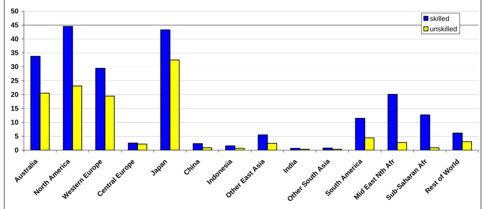
immigration records we used them to investigate the relationship between migration flows and stocks. The ratio of migrant flows to stocks was first calculated, as shown in Table 2, from which it can be seen that the ratios vary significantly across the destinations for each source region, yet the average ratio of immigration flows to stocks (the column ratios) are comparatively robust across the destination regions. As flow data for the remaining 11 regions is not readily or reliably available the average ratios for each region of origin were applied to the stock matrix to produce the resulting matrix of migration flows, presented in Table 3 and summarised in Figure 1.6

Our approximations suggest that the largest source of gross emigrants was “Central Europe and the Former Soviet Union” whose former residents tended to settle in Western Europe. The next largest source of gross emigrants was the “Rest of the World” grouping, which includes New Zealand, the former Yugoslavia and the Central American countries other than Mexico.7 The Central Europe and Former Soviet Union bloc was also the third most popular destination for migrants, following Western Europe and North America

respectively, with 22 per cent of the Central Europe and the Former Soviet Union immigrant intake coming from Sub-Saharan Africa.

Australia has the largest volume of immigrants by comparison with its population. The majority of these appear to come from the “Rest of the World” bloc, though Western Europeans account for 20 per cent of Australian annual immigration with Chinese and Other East Asians each providing roughly 10 per cent. On the other hand, 59 per cent of Australian emigration flows are to North America and Western Europe, with 13 per cent going to Central Europe and the Former Soviet Union and eight per cent to Asia.

6

Since immigration to developing region is likely to differ qualitatively from that into industrial regions, this assumption is likely to cause bias. There is as yet no clear evidence as to the direction of this bias, however.

7

Because the GTAP economic database offers a restricted list of regional aggregations, as shown in Table 1 the former Yugoslavia is allocated to the rest of the world group, as are the countries of Central America (excluding Mexico). During the 1990s these were key sources of immigrants to Western Europe and North America, respectively, which is why this region also appears to have offered the largest volume of net emigrants.

The regions with net annual immigration, as shown in Figure 1, are Western Europe, North America, Australia, the Middle East and North Africa, and Japan, in descending order of volume. All the remaining regions have net annual emigration rates with the Rest of the World providing the largest source of migrants and Indonesia the least.

Migration Flows by Age and Gender

Detailed accounts of both the regional and the age-gender compositions of immigrant flows are unavailable for most countries and regions. A comprehensive breakdown is

available for the United States, however, via the US Citizenship and Immigration Services (USCIS, 2001)8. It is therefore assumed that the age-gender composition of all migrant flows matches that of immigrants to the United States. By firstly summing the total US immigrant population of each group for the years 1986 to 2001, the migrant population share of each group was derived. These shares were then applied to the aggregate flow matrix of Table 3 to derive a set of eight matrices that detail the migrant flows between regions for each age-gender group. Thus the annual migration flow rate for age group a, gender g, from the region of origin r and to the destination in region d can be expressed algebraically as:

(2) , , , , , , , 60 , , , , , 014 a g r d NthAmerica r d R r a g r d f a g d a g r d NthAmerica r a g m M M M N M = + = = = ⎛ ⎞ ⎜ ⎟ ⎜ ⎟ = ⎜ ⎟ ⎜ ⎟ ⎝ ⎠

∑

∑ ∑ ∑

where is the annual migration flow rate between r and d expressed as a proportion of the destination region d’s group population, . The variable

, , , R a g r d M , , a g d

N Mr d, represents the total flow of migrants from r to d in Table 3 and is the age and gender specific flow of immigrants to North America.

, ,

a g d NthAmerica

M ₌

Our analysis divides production (unskilled) workers from professional (skilled workers). 9 Indeed, all age-gender groups are stratified in this way so as to represent socioeconomic division.10 To thus subdivide the matrices of migration flows we make the strong assumption that the matrix of age-gender specific migration rates, , is the same for production worker and professional migrant worker flows. Statistical evidence is

, , , R a g r d M 8

Thanks are due to Professor Tim Hatton of the Australian National University for directing the authors to these data.

9

Professional, or “Skilled” occupations include managers, professionals, engineers, scientists, teachers and bureaucrats, to list a few (Hertel, 1997). Production, or unskilled workers are defined to include tradespersons, clerks, sales assistants, industrial workers and farm hands (Liu et al, 1998).

10

The stratification even applies to children, on the grounds that the offspring of skilled parents are very likely to attain skill levels at least as advanced as their parents.

accumulating that indicates the contrary (Docquier and Marfouk, 2006), yet the available data remain insufficient to form a reliable separation between the two complete matrices of

migration rates.

3. The Incentive to Migrate - Regional Real Wage Differences

If we assume that the average quality of workers in each occupational group (production and professional workers) is the same across regions, then inter-regional real wage inequality must stem from differences in relative factor abundance and technology, combined with trade and migration restrictions (Tokarik, 2002). Trade liberalisation and skill-biased technical change have accelerated the growth in demand for professional relative to production labour in developed countries. This has tended to expand the wedge between the real wage rates of skilled and unskilled workforces, or to raise the “skill premium”. Conversely, the associated realisation of developing regions’ comparative advantage in

labour-intensive products has tended to raise production wage rates. In these regions, the pure trade effect has therefore been to reduce the skill premium, yet they, too, have encountered skill-biased technical change and so the net effect on skill premia in developing regions has depended on the relative magnitudes of these two effects (Suryahadi et al. 2001).

Wage inequality can also be related to international migration (Kar and Beladi, 2002). Most migration, as indicated in the previous section, is from less developed regions to the OECD countries. Depending on the skill-composition of the migration flows, they can be expected to reduce real production and professional wages in the destination regions while raising them in the regions of origin. It is our objective to estimate these effects using a global simulation model. To facilitate this, however, it is necessary to assemble a starting distribution of real wages across regions by skill level. The key resource for this analysis is the GTAP global database. In it, production (unskilled) and professional (skilled) labour are defined based on ILO occupational categories (Liu et al. 1998). The database offers total payments to each type of labour in each region for the base year, 1997. No adjustment is made in the database for purchasing power parity (PPP).

Market Exchange Rate Wages

The GTAP Database provides total payments to each of the two types of labour, denominated in US dollars at market exchange rates (MER). It does not offer volume statistics for primary factor inputs other than physical capital, however. Estimates are therefore required of total full time equivalent labour forces by skill level in each region.

Labour force numbers by age and gender were obtained from Chan and Tyers (2006) for the year 1997. Labour force shares of skilled workers were then obtained from Liu et al. for each GTAP-defined region, and then aggregated to the 14 applied here.

Wage rates in region r for skill level s, used for the purpose of this analysis were firms’ purchases at agents’ prices, EVFAs,r, which had been calculated as expenditure on

labour by firms across all sectors. Thus the 1997 US$ annual wage per worker, w, in region r for skill s was derived via:

(3) _{, 60} , , , , , 1539 s skilled r MER s skilled r f a g r a g r a g m EVFA w L S = = + = = =

∑ ∑

∑ ∑

where for age a and gender g is the size of the full time equivalent labour force and is the volume share of skilled labour. The resulting rates are listed in Table 4 and plotted in Figure 2. r g a L , , , , a g r S

These results indicate that the US$ rewards to workers in 1997 were highest in the industrialised regions while developing regions, typically with higher population densities and poorer technologies, have lower wages for both skilled and unskilled workers. There are also significant wage differences between the skill levels for all regions with professional workers earning consistently more than production workers11. The lowest wage rate for production workers was in the Indian and Other South Asian regions, with workers earning roughly US$350 per year, while Japan offered its production workers the largest unskilled reward at a rate of US$32,449 per year. North America and Japan payed professional workers the highest wage at more than US$43,000 per year whereas India offered its professional workers the lowest compensation at an average wage of approximately US$650 per year.

It is notable that the coefficient of inter-regional variation in average production wages is larger than the corresponding coefficient for professional wages (Table 4). One hypothesis to explain this is that the global markets for professional workers are more integrated via skilled migration than are those for unskilled workers.

The implicit assumption behind the assembly of the GTAP global database is that the purchasing power of one US$ is equal in all regions. For most applications, departures from this assumption do little harm. In considering migration inducement, however, the fact that the prices of non-tradables in developing countries are lower than in industrial countries implies that the purchasing power of a US$ is higher in the developing countries. Since

11

This is with the exception of Central Europe and the Former Soviet Union which appears to have had slightly larger returns to production labour. This is very likely a statistical aberration due to inaccurate national accounts data on labour payments.

inducement to migrate depends at least in part on the real purchasing power of wages in destination and origin regions, errors in MER-based projections of real wages tend to cause overestimation of the migration response. Purchasing power parity (PPP) wages would more reliably reflect the true distribution because they would incorporate, at least partly, a more realistic valuation of non-traded goods and services.

PPP-adjusted wages

In order to compare the real purchasing power of wages across regions, the market exchange rate results in Table 4 were converted to PPP using a multiplier derived the Global Development Network Database (World Bank, 2000). This multiplier is the ratio of the MER-based GDP estimate in US$ to the corresponding PPP estimate, by country in 199712. This was used to calculate the PPP multiplier for that year, α_rPM, for the 14 defined regions, by aggregating individual countries according to MER-based GDP shares. The PPP wage estimates are therefore:

(4) w_{s r}PPP_, =w_{s r}MER_, α_rPM, where . PPP MER PPP MER i i r MER MER i r i j j r GDP GDP GDP GDP α ∈ ∈ ⎛ ⎞ ⎜ ⎟ = _⎜ ⋅ _⎟ ⎜ ⎟ ⎝ ⎠

∑

_∑

and and represent, respectively, the GDP corresponding to purchasing power parity and market exchange rate values in country i.

PPP i

GDP MER

i

GDP

PPP wage results are also listed Table 4. They indicate a smaller wage range across regions for both skilled and unskilled workers when compared with MER values. The

coefficient of variation of production wages per worker decreased from the MER ratio of 1.32 to 0.97. Similarly, the PPP professional wage rate also had a reduced coefficient of variation, down from the MER value of 1.11 to 0.80. Average regional PPP-adjusted wages were larger by approximately US$619 for production workers and US$3,478 for professional workers. In developing regions, average PPP-adjusted wages doubled for production workers and more than doubled for professional workers. These revised wage divergences notwithstanding, no significant changes in the regional rankings of wages are suggested and so the implications of PPP adjustment would not appear to affect preferred migration directions.13 For the present at least, our subsequent analysis is therefore based on MER-based real wage divergences.

12

Thanks are due to Prof. Steve Dowrick of the Australian National University for directing the authors to these data.

13

One anomaly concerns the professional wage in Sub-Saharan Africa, which is very high PPP-adjusted. While it is possible that the comparatively small number of professionals in this region do have extraordinarily high real incomes, it is likely that the large value is inflated by undercounting. Moreover, other lifestyle

4. Modelling Global Economic and Demographic Change

The approach adopted follows Tyers et al. (2005), in that it applies a complete demographic sub-model that is integrated within a dynamic numerical model of the global economy. The economic model is a development of GTAP-Dynamic, the standard version of which has single households in each region and therefore no demographic structure.14 The version used has regional households that are disaggregated by age group, gender and skill level.

4.1 Demography:

The demographic sub-model tracks populations in four age groups and two genders: a total of 8 population groups in each of 14 regions.15 The four age groups are the dependent young, adults of fertile and working age, older working adults and the mostly-retired over 60s. The resulting age-gender structure is displayed in Figure 3. The population is further divided between households that provide production labour and those providing professional labour.16 Each age-gender-skill group is a homogeneous sub-population with group-specific birth and death rates and rates of both immigration and emigration.17 If the group spans T years, the survival rate to the next age group is the fraction 1/T of its population, after group-specific deaths have been removed and its population has been adjusted for net migration.

The final age group (60+) has duration equal to measured life expectancy at 60, which varies across genders and regions. The key demographic parameters, then, are birth rates, sex ratios at birth, age and gender specific death, immigration and emigration rates and life expectancies at 60.18 Immigration rates are a particular focus here and these are responsive to inter-regional real wage comparisons, constrained in a manner designed to represent the impacts of immigration policy. A further key parameter is the rate at which each region’s education and social development structure transforms production worker families into professional worker families. Each year a particular proportion of the population in each

14

The GTAP-Dynamic model is a development of its comparative static progenitor, GTAP (Hertel et al. 1997). Its dynamics is described by Ianchovichina and McDougall (2000). The adaptation of the model to incorporate the demographic sub-model is detailed in Tyers and Shi (forthcoming a).

15

The demographic sub-model has been used in stand alone mode for the analysis of trends in dependency ratios. For a more complete documentation of the sub-model, see Chan and Tyers (2006).

16

The subdivision between production and professional labour accords with the ILO’s occupation-based classification and is consistent with the labour division adopted in the GTAP Database. See Liu et al. (1998).

17

Mothers in families providing production labour are assumed to produce children that will grow up to also provide production labour, while the children of mothers in professional families are correspondingly assumed to become professional workers.

18

Immigration and emigration are also age and gender specific. The model represents a full matrix of global migration flows for each age and gender group. Each of these flows is currently set at a constant proportion of the population of its destination group. See Chan and Tyers (2006) and Vedi (2005) for further details.

production worker age-gender group is transferred to professional status. These proportions have an exogenous component that is set depending on the regions’ levels of development, the associated capacities of their education systems and the relative sizes of the production and professional labour groups. They are also responsive to regional skilled wage premia, to an extent that is readily adjusted to reflect changes in the capacities of education and training systems.

In any year, for each age group, a, gender group g, skill group s, region of origin, r and region of destination, d, the volume of migration flow is:

(5) M_{a g s r d}t_{, , , ,} =δ_dtM_{a g s r d}R_{, , , ,} N_{a g s d}t_{, , ,} , ∀a g r, , ,d ,

where δ_dt is a destination-specific factor reflecting immigration policy in region d, set to unity in all but counterfactual experiments, is the migration rate between r and d expressed as a proportion of the group population in region d, . The migration rate is then responsive to regional differences in real wages via:

R agsrd M agsd N (6) , , , , , , 0 , , , , , , , , M a g s r d s d s r R R a g s r d a g s r d C C d r W W M M P P ε ⎡⎛ ⎞ ⎛ ⎞⎤ = _{⎢⎜ ⎟ ⎜ ⎟⎥} ⎝ ⎠ ⎝ ⎠ ⎣ ⎦ ,

where W_{s r,} and W_{s d,} are wage rates by skill level in regions of origin and destination

(measured relative to a common global numeraire), and are consumer price levels in the two regions (measured relative to the same global numeraire) and is an elasticity of response that reflects the extent to which immigration policies constrain the bilateral flow between r and d. C r P C d P , , , , M a g s r d ε

Given the migration matrix, , the population in each age, gender and skill group and region can be constructed. We begin with the population of males aged 0-14 from professional families in region d (a=014, g=m, s=sk, r=d).

agsrd M (7) 1 1 014, , , 014, , , , 1539, , , 1 014, , , 014, , , 014, , , , 014, , , , 1 1 1 014, , , 014, , , 014, , , 014, , , 1 1 , 15 t t t d t t m sk d m sk d t sk d f sk d d t t t t m sk d m sk d _r m sk r d _r m sk d r t t t t d m unsk d m sk d m sk d m sk d S N N B N S D N M M N N D N ρ − − − − − − = + + − + − ⎡ ⎤ + − _⎣ − _⎦

∑

∑

where S_dt is the sex ratio at birth (the ratio of male to female births) in region d, B_{s d}t_, is the birth rate for women of skill level sk, 014, , the death rate and

t m d

D ρd is the rate at which region

d’s educational institutions and general development transform production into professional worker families. The final term is survival to the corresponding 15-39 age group. In the

corresponding equation for young males from production worker families the penultimate term is negative and the subscript sk is replaced with unsk in all but that penultimate term.

For females in professional families in this age group the corresponding equation is:

(8) 1 1 014, , , 014, , , , 1539, , , 1 014, , , 014, , , 014, , , , 014, , , , 1 1 1 014, , , 014, , , 014, , , 014, , , 1 1 1 , 15 t t t t f sk d f sk d t sk d f sk d d t t t t f sk d f sk d _r f sk r d _r f sk d r t t t t d f unsk d f sk d f sk d f sk d N N B N S D N M M N N D N ρ − − − − − − = + + − + − ⎡ ⎤ + − _⎣ − _⎦

∑

∑

For adults of gender g from professional families in the age group 15-39 the equation includes a survival term from the younger age group. It is:

(9) 1 1 1 1539, , , 1539, , , 014, , , 014, , , 014, , , 1 1539, , , 1539, , , 1539, , , , 1539, , , , 1 1 1539, , , 1539, , , 1539, , , 153 1 15 1 25 t t t t t g sk d g sk d g sk d g sk d g sk d t t t t g sk d g sk d _r g sk r d _r g sk d r t t t d g unsk d g sk d g sk d N N N D N D N M M N N D N ρ − − − − − − ⎡ ⎤ = + _⎣ − _⎦ − + − + − −

∑

∑

where the second term is the surviving inflow from the 0-14 age group and the final term is the surviving outflow to the 40-59 age group. Again, the skill transformation term is negative in the case of the corresponding equation for production worker families. The population of professional adults of gender g, in age group 40-59 follows as:

(10) 1 1 1 4059, , , 4059, , , 1539, , , 1539, , , 1539, , , 1 4059, , , 4059, , , 4059, , , , 4059, , , , 1 1 4059, , , 4059, , , 4059, , , 1 25 1 20 t t t t t g sk d g sk d g sk d g sk d g sk d t t t t g sk d g sk d r g sk r d r g sk d r t t t d g unsk d g sk d g sk d N N N D N D N M M N N D N ρ − − − − − − ⎡ ⎤ = + _⎣ − _⎦ − + − + − −

∑

∑

For adults in the 60+ age group, the corresponding relationship is:

(11) 1 1 1 60 , , , 60 , , , 4059, , , 4059, , , 4059, , , 60 , , , , 60 , , , , 1 1 60 , , , 60 , , , 60 , , , 1 20 1 , , t t t t t g sk d g sk d g sk d g sk d g sk d t t g sk r d g sk d r r r t t d g unsk d t g sk d g sk d N N N D N M M N N L ρ − − − + + + + − − + + + ⎡ ⎤ = + _⎣ − _⎦ + − + − ∀

∑

∑

where the final term indicates that deaths from this group each year depend on its life

expectancy at 60, Lt_{60 , ,+g sk d,} . Again, the equation for aged production worker family members is the same except that the skill transformation term is negative.

Finally, ρ_d, the rate at which region d’s educational institutions and general

development transform production into professional worker households depends on the level of the region’s real GNP per capita and on the size of its skilled wage premium.

(12) 0 , , TW d sk d d d unsk d W W ε ρ =ρ ⎛⎜_⎜ ⎞⎟_⎟ ⎝ ⎠ , where 0 0 0 0 TY d TW TW d d d d C C d d d d GNP GNP N P N P ε ε =ε ⎛_⎜ ⎞_⎟ ⎝ ⎠ . TW d

ε is the elasticity of the transformation rate to the skilled-unskilled wage ratio. This elasticity is thought to be larger the more developed the region. To represent this, it is set to grow with real per capita GNP according to elasticityε_dTY.

Sources and structure:

Key parameters in the model are the migration rates, M_{a g s r d}R_{, , , ,} , birth rates, B_{s r}t_, , sex ratios at birth, S_rt, death rates, D_{a g s r}t_{, , ,} , life expectancies at 60, Lt_{60 , , ,+g s r} and the skill

transformation rates ρ_d. The migration rates are based on the flows analysed in Section 2. In the base line projection they are held constant through time – the elasticity is made negligibly small. The skill transformation rates are based on changes in the composition of aggregate regional labour forces as between production and professional workers during the decade prior to the base year, 1997, and on the human capital projections by Goujon and Lutz (2004). The resulting transformation rates are then refined so that, when they are held

constant through 2030, the skill premia in all regions remain stable. This then yields the base line projection. To maintain the base line constant transformation rates, the elasticities

, , , , M a g s r d ε TW d ε

and ε_dTY are made negligibly small.19

Asymptotic trends in other parameters:

The birth rates, life expectancy at 60 and the age specific mortality rates all trend through time asymptotically. For each age group, a, gender group, g, and region, r, a target rate is identified.20 The parameters then approach these target rates with initial growth rates determined by historical observation. In year t the birth rate of region r is:

(13) 0

(

)(

1

t t

r r Tgt r

)

B =B + B −B −eβ ,

where the rate of approach, β, is calibrated from the historical growth rate:

(14)

(

)(

)

Note that, as regions become more advanced and populations in the production worker families become comparatively small, constant skill transformation rates have diminishing effects on professional populations.

20

In this discussion the skill index, s, is omitted because birth and death rates, and life expectancies at 60 do not vary by skill category in the version of the model used.

(15) 0 0 0 0 ˆ ln 1 r r Tgt r B B B B β = ⎡_⎢ − ⎤_⎥ − ⎢ ⎥ ⎣ ⎦ .

Labour force projections:

To evaluate the number of “full-time equivalent” workers we first construct labour force participation rates, Pa,g,r by gender and age group for each region from ILO statistics on

the “economically active population”. We then investigate the proportion of workers that are part time and the hours they work relative to each regional standard for full time work. The result is the number of full time equivalents per worker, Fa,g,r. The labour force in region r is

then: (16) 60 , , , 1539 f unsk t t r a a g m s sk L + L = = = =

∑ ∑ ∑

Here µ_{a r}t_, is a shift parameter reflecting the influence of policy on participation rates. The time superscript on P_{a g r}t_{, ,} refers to the extrapolation of observed trends in these parameters.21

Asymptotic trends in labour force participation:

For each age group, a, gender group, g, and region, r, a target country is identified whose participation rate is approached asymptotically. The rate of this approach is determined by the initial rate of change. Thus, the participation rate takes the form:

(17) 0

(

)(

)

, , , , , , 1

t t

a g r a g r Tgt a g r

P =P + P −P −eβ ,

where the rate of approach, β, is calibrated from the initial participation growth rate:

(18)

(

)(

)

Target rates are chosen from countries considered “advanced” in terms of trends in

participation rates. Where female participation rates are rising, therefore, Norway provides a commonly chosen target because its female labour force participation rates are higher than for other countries.22

Accounting for part time work:

21

Although part time hours may well also be trending through time, we hold F constant in the current version of the model.

22

For each age group, a, gender, g, and region, r, full-time equivalency depends on the fraction of participants working full time, fa,g,r, and, for those working part time, the ratio of

average part time hours to full time hours for that gender group and region, rg,r. For each

group, the ratio of full time equivalent workers to total labour force participants is then (20) Fa g r, , = fa g r, , + −

(

)

23

The aged dependency ratio:

We define and calculate four dependency ratios: 1) a youth dependency ratio is the number of children per full time equivalent worker, 2) an aged dependency ratio is the number of persons over 60 per full time equivalent worker, 3) a non-working aged dependency ratio is the number of non-working persons over 60 per full time equivalent worker, and 4) a more general dependency ratio is defined that takes as its numerator the total non-working population, including children.24 That used here is the one of most widespread policy interest, the non-working aged dependency ratio:

(21)

(

)

∑ ∑

4.2 The Global Economic Model

GTAP-Dynamic is a multi-region, multi-product dynamic simulation model of the world economy. It is a microeconomic model, in that assets and money are not represented and prices are set relative to a global numeraire. In the version used, the world is subdivided into 14 regions. Industries are aggregated into just three sectors, food (including processed foods), industry (mining and manufacturing) and services. To reflect composition differences

between regions, these products are differentiated by region of origin, meaning that the “food” produced in one region is not the same as that produced in others. Consumers substitute imperfectly between foods from different regions.

As in most other dynamic models of the global economy, in GTAP-Dynamic the endogenous component of simulated economic growth is physical capital accumulation. Technical change is introduced in the form of exogenous trends and skill (or human capital) acquisition is driven by the constant transformation rates introduced in the previous section.

23

Preliminary estimates of fa,g,r and rg,r are approximated from OECD (1999: Table 1.A.4) and OECD (2002: Statistical Annex, Table F). No data has yet been sought on part time work in non-OECD member countries. In these cases the diversity of OECD estimates is used to draw parallels between countries and regions and thus to make educated guesses. The results are listed by Chan and Tyers (2006: Tables 11 and 12).

24

A consequence of this is that, at least for the world as a whole, the model exhibits the property that an increase in the growth rate of the population raises the growth rate of real GDP but reduces the level of real per capita income. This result is common to all such models where there are diminishing returns to capital and labour, the simplest of these models being that of Solow (1956) and Swan (1956), the effects of population growth in which are detailed by Pitchford (1974: Ch.4). What distinguishes the model from these simpler progenitors is its recursive multi-regional dynamics. Investors have adaptive expectations about the real net rates of return on installed capital in each region. These drive the distribution of investment across regions. In each, the level of investment is determined by a comparison of net rates of return with borrowing rates yielded by a global trust to which each region’s saving

contributes.

To capture the full effects of demographic change, including those of ageing, the standard model has been modified to include multiple age, gender and skill groups in line with the structure of the demographic sub-model. In the complete model, these 16 groups differ in their consumption preferences, saving rates and their labour supply behaviour. Unlike the standard GTAP models, in which regional incomes are split between private consumption, government consumption and total saving via an upper level Cobb-Douglas utility function that implies fixed regional saving rates, this adaptation first divides regional incomes between government consumption and total private disposable income. The implicit assumption is that governments balance their budgets while private groups save or borrow.

In splitting each region’s private disposable income between the eight age-gender groups, the approach is to construct a weighted subdivision that draws on empirical studies of the distribution of disposable income between age-gender groups for “typical” advanced and developing countries.25 Individuals in each age-gender group then split their disposable incomes between consumption and saving. For this a reduced form approach is taken to the intertemporal optimisation problem faced by each. It employs an exponential consumption equation that links group real per capita consumption expenditure to real per capita disposable income and the real interest rate. This equation is calibrated for each group and region based on a set of initial (1997) age-specific saving rates from per capita disposable income.26 Importantly, these show transitions to negative saving with retirement in the older industrial regions. This gives rise to declines in average saving rates as population’s age. The empirical studies on age-specific saving behaviour are less clear, however, when it comes to developing regions. In the important case of China, for example, only modest declines in saving rates are

25

The analytics of income splitting are described in detail by Tyers et al. (2005).

26

recorded when people retire. This is partly due to complications associated with China’s transformation from state to private employment and, of wider relevance to developing countries, the comparatively large proportion of elderly consumption spending that is financed from the income of younger family members (Feng and Mason 2005).

5. Constructing the Base Line Scenario

The base line scenario represents a “business as usual” projection of the global economy through 2030. Although policy analysis can be sensitive to the content of this scenario, the focus of this paper is on the extent of departures from it that would be caused by alternative levels of responsiveness of migration flows to inter-regional real wage divergences.

Nonetheless, it is instructive to describe the base line, because all scenarios examined have in common a set of assumptions about future trends in productivity and because some exposition of the base line makes the construction of departures from it clearer.

Exogenous factor productivity growth

Exogenous sources of growth enter the model as factor productivity growth shocks, applied separately for each of the model’s five factors of production (land, physical capital, natural resources, production labour and professional labour). Simulated growth rates are very sensitive to productivity growth rates since, the larger these are for a particular region the larger is that region’s marginal product of capital. The region therefore enjoys higher levels of investment and hence a double boost to its per capita real income growth rate. The importance of productivity notwithstanding, the empirical literature is inconsistent as to whether productivity growth has been faster in agriculture or in manufacturing and whether the gains in any sector have enhanced all primary factors or merely production labour. The factor productivity growth rates assumed in all scenarios are drawn from a new survey of the relevant empirical literature (Tyers et al. 2005). Agricultural productivity grows more rapidly than productivity in the other sectors in China, Indonesia, Other East Asia, India and Other South Asia. This allows continued shedding of labour to the other sectors. In the

industrialised regions, the process of labour relocation has slowed down and labour productivity growth is slower in agriculture.

Interest premia

The standard GTAP-Dynamic model takes no explicit account of financial market maturity or investment risk and so tends to allocate investment to regions that have high marginal

products of physical capital. These tend to be labour-abundant developing countries whose labour forces are still expanding rapidly. Although the raw model finds these regions attractive prospects for this reason, we know that considerations of financial market

segmentation, financial depth and risk limit the flow of foreign investment at present and that these are likely to remain important in the future. To account for this we have constructed a “pre-base line” simulation in which we maintain the relative growth rates of investment across regions. In this simulation, global investment rises and falls but its allocation between regions is thus controlled.27 This creates wedges between the international and regional borrowing rates. They show high interest premia for the populous developing regions of Indonesia, India, South America and Sub-Saharan Africa. Premia tend to fall over time in other regions, where labour forces are falling or growing more slowly. Most spectacular is a secular fall in the Chinese premium, due to the maintenance of investment growth in China despite the eventual slow-down and decline in its labour force.28 In the subsequent base line simulation, and in all other simulations, investment levels are again set as endogenous and the time paths of all interest premia are made exogenous.

The base line projection

Demographic changes in the base line projection are characterised by declining fertility and ageing in all regions. The key demographic differences between regions concern their initial age distributions and fertility levels – the industrialised regions begin with older populations and lower fertility than the developing ones and so, generally, population growth continues to be higher in the developing regions, particularly in South Asia and Africa, as shown in Figure 4. The pervasive ageing is suggested by the projected sizes and

compositions of regional labour forces listed in Table 5 and the non-working aged

dependency ratios in Table 6. Economic changes in the base line are indicated in Table 7, which details the average GDP and real per capita income growth performance of each region from 1997 to 2030. In part because of its comparatively young population and hence its continuing rapid labour force growth, India attracts substantial new investment and is projected to take over from China as the world’s most rapidly expanding region. Rapid population growth detracts from India’s real per capita income performance, however. By this criterion, China is the strongest performing region through the three decades. Indonesia and “other East Asia” are also strong performers, while the older industrial economies

27

To do this the interest premium variable (GTAP Dynamic variable SDRORT) is made endogenous, only in the pre-base simulation.

28

continue to grow more slowly. The African regions enjoy good GDP growth performance but their high population growth rates limit their performance in per capita terms.

6. Increasing Responsiveness to Real Wage Divergences

The shocks introduced centre on the elasticities in equations (6) and (12). Recall from (6) that is the elasticity of the migration rate for skill level s between regions r and d to the ratio of the destination and origin real wages. In the base line simulation, this elasticity is set to negligibility, so that migration flows are driven only by the sizes of destination populations in each age-gender group. That is, flows maintain base period rates of immigration over destination populations in each bilateral direction for each age-gender group. This is intended to imply that the flows are dictated by immigration policies in destination regions and thus regulated on adaptation cost grounds.

, , , , M a g s r d ε

The high migration simulations

The first alternative simulation, labelled M1, simply expands this elasticity, for skilled workers only, to a value of 0.5 in the interval 2000-2010.29 Skilled migration volumes then increase by most between low and high real wage regions. Because this additional migration makes skilled workers scarcer in the regions of origin, however, the skill premium rises in those regions. This might be expected to induce a skill-acquisition response from production workers in the regions of origin. Allowance for accelerated skill transformation takes the form of (12), in which εTWd is the elasticity of the transformation rate to the ratio of skilled and production real wages and ε_dTY governs the response of ε_dTW to rising real per capita incomes and hence rising educational opportunity and is set at unity throughout. εdTWis set at

negligibility in the base line and in M1, so that skill transformation rates are constant through time for each region.

A second alternative simulation is constructed that is the same as M1 except that accelerated skill transformation is allowed by adjusting ε_dTW. More particularly, the new simulation, labelled M2, has εTWd rising to a value of 0.25 over 2000-2010. This enlargement enables responses to pre-existing skill premia as well as to changes in skill premia induced by altered immigration policies. Where skill premia are large at the outset, as is most notably the case in North America and Africa (Figure 2), skill acquisition can therefore be expected to accelerate most. The base line and M2 values of the transformation rates are listed in Table 8.

29

Rates are initially small in all regions, expanding most, as expected, in North America and Africa.

Increasing responsiveness to real wage divergences

Expanding migration in a manner that is responsive to real wage differences is found to yield “more of the same” in terms of the direction of and relative magnitudes of migration flows. This is reassuring in that it suggests that real wage divergences are an explanation for recorded migration, immigration policies and quotas notwithstanding. The similarity of pattern is clear from a comparison of the base period annual flows, indicated in Figure 1, with the accumulation of projected flows over the next three decades shown in Figure 5. Except in the cases of two prominent regions of origin, Central Europe and the former Soviet Union and the “rest of the world” group, migrants tend to leave populous regions, so that their departures have small proportional effects. As is clear from Figure 6, however, they do make a

significant difference in the principal regions of destination, namely Western Europe, North America and Australia.30 Of the destination regions identified, the skilled immigrant intake is largest relative to the population in Australia, where the additional migrants expand the 2030 population by almost a tenth.

The economic effects of these migrant flows come from changes in skilled labour forces and, because the migrants tend to be younger than the average age in destination regions, these imply associated changes in non-working aged dependency ratios. The labour force effects are illustrated in Figure 7 and detailed in Table 9. The professional labour forces of Western Europe, North America and Australia are raised by between a tenth and a quarter, while those of the key regions of origin fall. The corresponding effects on aged dependency are smaller, however. Considering that migrants are younger on average than destination populations and that the three-decade increases in the base line destination labour forces are large (Table 6), the 2030 destination non-working aged dependency ratios fall by small amounts - a fraction of a per cent in Western Europe, a per cent or so in North America and nearly two per cent in Australia (Table 10). Clearly, the age distribution effects are modest and expanded skilled migration is unlikely to be a solution to the fiscal problems associated with age dependency.31

30

The Middle East and North Africa is also a prominent destination region, particularly for workers from South and Southeast Asia, but this migration remains small in relation to the population of that region.

31

This is a well-established conclusion in demography (Young, 1990) that has been re-examined following the rise in concern about population ageing and slower growth in Europe (United Nations 2000a). A clearer demonstration of it using the method of this paper can be found in Tyers and Shi (forthcoming b).

The expanded professional labour forces in the principal destination regions do have broader economic implications, however. Although their effects on the average growth rates of GDP over three decades are small compared with the drivers of base line growth (Figure 8), the economies of the destination regions are larger than their base line levels by between two and eight per cent in 2030 (Figure 9). For the world as a whole, the migrations raise 2030 global GDP by 1.6 per cent. The assumed homogeneity of professional workers across

regions and the market exchange rate database of the GTAP-Dynamic model, which tends to make labour productivity in tradeable goods sectors more similar than the actual wage data of Section 3 suggest, both act to reduce the estimated global GDP gains from the relocation of skilled workers.

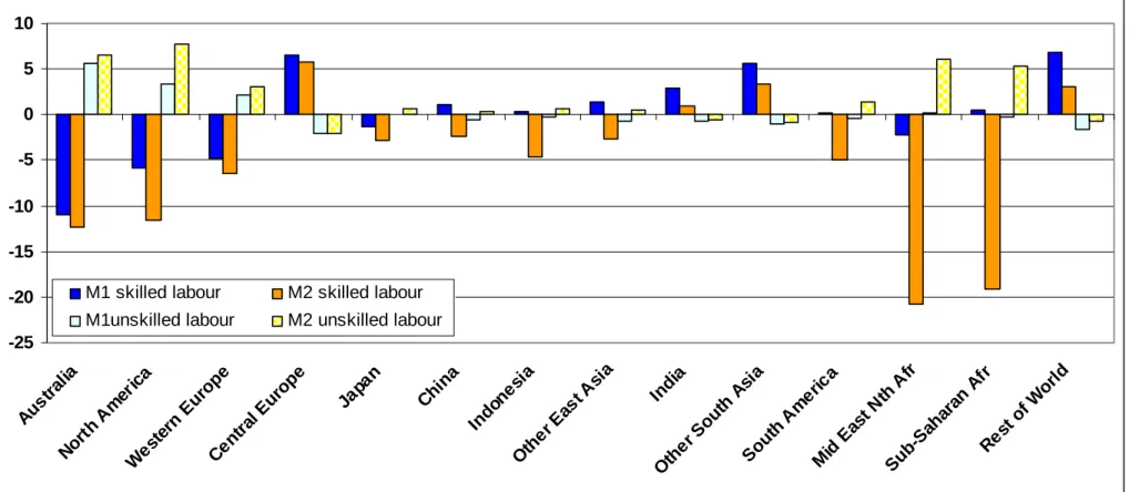
The impacts of increased migration on wages are shown in Figure 10. They are straight-forward. In M1, where there is no change in the rate of skill acquisition within regions, real professional wages fall in destination regions, which experience increased professional labour supply, and rise in regions of origin. Production wages rise in the destination regions, since the rise in the supply of skill raises the marginal product of

production labour there. The opposite is true in regions of origin, where the skill supply falls. It is also evident from Figure 10 that the skill premium falls in the destination regions and rises in the regions of origin. Even though the labour forces of India and “other South Asia” are very large by comparison with their emigrations, their skilled labour forces are reduced by measurable proportions (Figure 7). This causes significant increases in their skilled wage rates relative to the base line projection, as shown in Figure 10 and listed in Table 11. The corresponding changes in East and Southeast Asia are smaller because skilled wages are higher there at the outset and so proportionally smaller emigrations are induced.32

Finally, the net effects of all this on populations, the skill intensity of labour forces, terms of trade and real per capita income are indicated in Table 12. The migration-only effects on destination regions, from M1, are three-fold. First, immigration raises the domestic population, slowing the growth rate of real income per capita (following the behaviour of all such neoclassical capital-accumulation models, as discussed in Section 4.2).33 Second, the skill level of the overall labour force is increased by the immigration, which tends to raise real income per capita and hence to at least partially offset the population effect. Third,

32

The pattern for the “Middle East and North Africa” is reversed, of course, because this region is a destination for migrants due to its concentrations of petroleum wealth, even though it includes many poor countries.

33

As Pitchford (1974), indicates, technical change assumptions are important in this. In our analysis the underlying changes in factor productivity are exogenous and constant across the base line, M1 and M2

simulations. This absence of interaction between migration and the productivity of individual factors (including production and professional labour) ensures that the standard implications of population growth for per capita income emerge.

destination regions have lower average real wages and hence lower production costs and export prices relative to regions of origin. They therefore experience real depreciations relative to the base line, or adverse terms of trade effects.34 These three effects tend to offset each other, so that the net changes in real per capita income due to expanded skilled migration are small.

In Australia, because of the dominance of the population-expanding and terms of trade effects, real per capita income is shown to grow slower, ending up lower in 2030 by more than a per cent. In North America, the (negative) population expansion effect is smaller by more than half, while the (positive) skill intensity and (negative) terms of trade effects are smaller by just over a third. On net, then, North America is a small gainer form the expanded immigration. In the case of Western Europe, all three effects are smaller still, and the net is a very small loss relative to the baseline. Japan is a small net gainer, mainly because of an externally induced improvement in its terms of trade. In most source regions, the slower population growth due to emigration, combined with their improved terms of trade, dominates their loss of skill intensity, so they are net gainers. The exceptions are “other South Asia”, which suffers a substantial reduction in skill intensity, and Sub-Saharan Africa, where all three effects are proportionally small but the loss of skill intensity appears to dominate.

Increasing both migration and skill-acquisition responsiveness

When the additional effect of skill acquisition is added, in M2, net migration movement is slightly larger (Figure 5). This is so because the skill-acquisition reduces the tendency for the migration to raise professional wages and skill premia in regions of origin by more than it lowers professional wages, and hence squeezes skill premia, in destination regions. Evident from the real wage changes in Figure 10, this is due to the expansion in skill acquisition responding more to pre-existing skill premia than to changes associated with migration. In the regions of origin the rates of skill acquisition expand more markedly, as shown in Table 8. The most pronounced effects are in the poorest regions, where the skill premia were extremely high in 1997 (Figure 2). For this reason, the wage of professional workers falls by most in the Middle East and North Africa and in Sub-Saharan Africa. It falls by more modest yet significant proportions in South America and in East and Southeast Asia, where this constitutes a reversal of the effects of pure skilled migration (M1). That reversal is due to the dominance over skilled wage determination by the domestic skill transformation process, with its enhanced sensitivity to high domestic skill premia, rather than by emigration.

34

For some regions, particularly those where the labour force size effects of the expanded migration are small, the terms of trade effects are driven mainly by externally induced changes in trading prices.

The increased skill endowments further boost GDP in the destination regions. This time, however, as Figure 9 shows, the change in skill composition in some regions of origin outweighs the effect of emigration and so also raises their GDP levels.

Returning to the declines in skill premia in the principal destination regions, the extent of this is, understandably, quite sensitive to the real wage divergence elasticity, . To minimise arbitrariness, we have shocked this elasticity to the same level (0.5) on all bilateral migration links. Too large an increase in this elasticity (say to a value of unity) causes the collapse of skill premia, first in Australia, where the proportional effects of the migrations are largest. The scale of the wage convergence embodied in the results shown in Figure 10 is further elucidated in Figure 11. In Australia, the skill premium is reduced in proportion, though not in level, while in North America and Western Europe, it is merely stabilised in proportion. Convergence of wage rates between regions, however, remains very modest, even with this substantial increase in skill migration flows (Table 11). All this suggests that global labour markets offer scope for still further expansions in skilled migration.

, , , , M a g s r d ε

35

Finally, the expanded skill-acquisition rates in M2 ensure that there are gains in real per capita income in all regions, relative to M1. As Table 12 indicates, skill intensity effects are uniformly larger or less negative, while population expansion and terms of trade effects are little different. Not surprisingly, these extra gains are largest in the Middle East and in Africa, where the initial skill premia are highest. Small net losses continue to be incurred by Australia, because of its comparatively large population expansion, and “other South Asia”, due to its skill depletion.

7 Conclusion

To investigate the effects of demographic changes on labour markets and the global distribution of economic growth, a new demographic sub-model is integrated with an adaptation of the GTAP-Dynamic global economic model. Skilled migration flows are assumed to be motivated by real wage differences to an extent that is variably constrained by immigration policies. A uniform relaxation of these constraints on all inter-regional

migration flows is found to have most effect on labour markets in the traditional migration destinations, Australia, Western Europe and North America, where it restrains the skill premium and substantially enhances GDP growth. The skill premium is raised, however, in regions of origin, and particularly in South Asia, although the extent of this is shown to

35

That there is scope for further expansion in skilled migration is also a conclusion by Hatton and Williamson (2005).

depend sensitively on the assumed responsiveness of skill acquisition to regional skill premia. In regions where skill premia are high at the outset, such as in North America, the Middle East and Africa, skill acquisition has a larger effect on regional wages than does migration.

The effects of expanded skilled migration on real per capita incomes depend on its implications for population sizes, labour force skill shares and the international terms of trade. As it turns out, these different effects tend to be off-setting in both regions of origin and

destination, so that net changes in real per capita incomes are proportionally small. Four important caveats must be borne in mind. First, our base period matrices of migration flows leave room for improvement, since, given the paucity of standardised migration data, their construction depends on numerous assumptions. New research on the documentation of migration stocks and flows will soon render some of those assumptions unnecessary. Second, because our flow matrices are constructed from corresponding matrices of migrant stocks that are based originally on census data, there is no distinction between short- and long-stay migrants. The migration matrices include both immigration and

emigration flows for each region, however, so this is not an important demographic issue. Its economic importance stems from the tendency for temporary migrants to remit incomes in a manner not accounted for in this study.

Third, our model depends heavily on the GTAP global database, which takes incomplete account of inter-regional variations in the pricing of goods and services that are costly to trade. Indeed, in the standard version of the model the levels of wages and of factor endowments do not need to be made explicit. This means that inter-regional differences in factor productivity are imperfectly accounted for and PPP adjustments are needed in

modelling the motive for migration. We have blended the standard database with additional information about labour supplies and wage levels to make possible our analysis of increases in the responsiveness of migration flows to wage divergences. In the long run, a more

systemic solution to this problem is required. Finally, although there is evidence to support it, we do not allow the fertility of professional households to depart from that of production worker households. Since a perception that skilled households have reduced fertility is an important aspect of the motivation for skill shortage claims, further research on the topic might better account for variations not only in fertility but also in other demographic parameters by the professional status of households.