Topics In Multivariate Statistics

University of Pennsylvania

ScholarlyCommons

2017

Topics In Multivariate Statistics

Xin Lu Tan

University of Pennsylvania, [email protected]

Follow this and additional works at:https://repository.upenn.edu/edissertations

Part of theStatistics and Probability Commons

This paper is posted at ScholarlyCommons.https://repository.upenn.edu/edissertations/2602

For more information, please [email protected].

Recommended Citation

Tan, Xin Lu, "Topics In Multivariate Statistics" (2017).Publicly Accessible Penn Dissertations. 2602.

Topics In Multivariate Statistics

Abstract

Multivariate statistics concerns the study of dependence relations among multiple variables of interest. Distinct from widely studied regression problems where one of the variables is singled out as a response, in multivariate analysis all variables are treated symmetrically and the dependency structures are examined, either for interest in its own right or for further analyses such as regressions. This thesis includes the study of three independent research problems in multivariate statistics.

The first part of the thesis studies additive principal components (APCs for short), a nonlinear method useful for exploring additive relationships among a set of variables. We propose a shrinkage regularization approach for estimating APC transformations by casting the problem in the framework of reproducing kernel Hilbert spaces. To formulate the kernel APC problem, we introduce the Null Comparison Principle, a principle that ties the constraint in a multivariate problem to its criterion in a way that makes the goal of the multivariate method under study transparent. In addition to providing a detailed formulation and exposition of the kernel APC problem, we study asymptotic theory of kernel APCs. Our theory also motivates an iterative algorithm for computing kernel APCs.

The second part of the thesis investigates the estimation of precision matrices in high dimensions when the data is corrupted in a cellwise manner and the uncontaminated data follows a multivariate normal

distribution. It is known that in the setting of Gaussian graphical models, the conditional independence relations among variables is captured by the precision matrix of a multivariate normal distribution, and estimating the support of the precision matrix is equivalent to graphical model selection. In this work, we analyze the theoretical properties of robust estimators for precision matrices in high dimensions. The estimators we analyze are formed by plugging appropriately chosen robust covariance matrix estimators into the graphical Lasso and CLIME, two existing methods for high-dimensional precision matrix estimation. We establish error bounds for the precision matrix estimators that reveal the interplay between the dimensionality of the problem and the degree of contamination permitted in the observed distribution, and also analyze the breakdown point of both estimators. We also discuss implications of our work for Gaussian graphical model estimation in the presence of cellwise contamination.

The third part of the thesis studies the problem of optimal estimation of a quadratic functional under the Gaussian two-sequence model. Quadratic functional estimation has been well studied under the Gaussian sequence model, and close connections between the problem of quadratic functional estimation and that of signal detection have been noted. Focusing on the estimation problem in the Gaussian two-sequence model, in this work we propose optimal estimators of the quadratic functional for different regimes and establish the minimax rates of convergence over a family of parameter spaces. The optimal rates exhibit interesting phase transition in this family. We also discuss the implications of our estimation results on the associated simultaneous signal detection problem.

Degree Type

Dissertation

Degree Name

Graduate Group Statistics First Advisor Andreas Buja Second Advisor Zongming Ma Subject Categories

TOPICS IN MULTIVARIATE STATISTICS Xin Lu Tan

A DISSERTATION in

Statistics

For the Graduate Group in

Managerial Science and Applied Economics

Presented to the Faculties of the University of Pennsylvania in

Partial Fulfillment of the Requirements for the Degree of Doctor of Philosophy

2017

Supervisor of Dissertation

Andreas Buja

Liem Sioe Liong/First Pacific Company Professor of Statistics

Co-Supervisor of Dissertation

Zongming Ma

Associate Professor of Statistics

Graduate Group Chairperson

Catherine Schrand

Celia Z. Moh Professor of Accounting

Dissertation Committee

Lawrence D. Brown

Miers Busch Professor of Statistics Abba M. Krieger

Robert Steinberg Professor of Statistics Po-Ling Loh

Assistant Professor of Electrical and Computer Engineering University of Wisconsin-Madison

TOPICS IN MULTIVARIATE STATISTICS

© COPYRIGHT

2017

Acknowledgments

I would like to start by thanking my advisors, Professor Andreas Buja and Professor Zongming Ma. Andreas instilled within me the virtues of deep and intuitive under-standing of problems as well as the importance of healthy skepticism in research. With his patience, guidance, and generous sharing of life wisdoms, Andreas guided me through a lot of hurdles in my Ph.D. study and helped me embrace my innate strengths as a researcher. In addition, Andreas inspired me with his immense curios-ity and openness in learning new subjects, and his tenaccurios-ity in pursuing formulation and solution of problems that are both elegant and fundamental. His high standards in writing and publishing had also time and again pushed me to go above and beyond my self-presumed limits. Andreas also has an exuberant and playful persona that I personally enjoy. On the other hand, Zongming piqued my interest in functional analysis and the theory of multivariate statistics. He encouraged me to make several moves that had since became keys in shaping my current Ph.D. portfolio. He is also generous in sharing perspectives and in offering advice when I am in doubt. Andreas and Zongming, thank you so much for willing to come together and work with me on topics that may be new to you as well. Thank you so much for encouraging me to explore broadly rather than to specialize prematurely in research. I am grateful

for the time we spent together studying functional principal component analysis and reproducing kernel Hilbert spaces, and for the many fun-filled conversations we had on a diverse range of topics. The time and memories we shared will always remain in my mind.

I would next like to thank Professor Tony Cai for introducing me to the mini-max framework of statistical thinking, and for guiding me throughout our study of quadratic functional estimation. His keen acumen, extensive knowledge and dedica-tion to research have made working with him an enjoyable learning experience.

My special thanks go to Professor Po-Ling Loh, who has been a friend, a mentor, and a role model to me. She gave me invaluable support, encouragement and com-panionship during our overlapping years. Po-Ling, the opportunity to attend your wedding has been an extremely illuminating experience as it prompted me to start contemplating who I want to be as I transition into adulthood. You are a truly inspir-ing person and I am very grateful for our friendship and for our research collaboration in robust statistics.

I would also like to thank the rest of my committee members, Professor Abba Krieger and Professor Larry Brown. Abba, thank you so much for working with me on the model selection probability project over one of my summers at Penn. Having TA’ed for you twice, I am also inspired by the deep care you showed on students learning. Larry, thank you so much for tossing out the problem of model selection probability estimation. Your relentless enthusiasm for research and devotion to the development of the statistical community are great exemplifications of scholarly spirit and are nothing short of inspirational.

Additionally, I would like to thank Professor Mark Low for admitting me to the program, without which this journey would not have been possible.

many professors with whom I have interacted, thank you so much for your friendliness, time, and advice. To our wonderful staff, thank you so much for the boundless support you provided, including assistance in room scheduling, package tracking, computing, conferences reimbursement, doctoral program logistics, and so much more. To the friends whom I had the pleasure of meeting during my Ph.D. study, including my cohort-mates (Zijian, Sam, Peichao, Dan, Tengyuan), and other students with whom I have overlapped, thank you for your camaraderie and friendship. Your companionship has made my life during Ph.D. study so much more enjoyable.

Last, but not least, I would like to thank my parents, Chiam Hua Tan and Ai Sian Teo, and my aunt, Sarah Teo, for believing in me and for unconditionally loving me. Thank you for being supportive of my education decision, and for always being there for me through times of joy and times of hardship. No matter what life may throw at me, I know I will always have your unwavering love and support.

ABSTRACT

TOPICS IN MULTIVARIATE STATISTICS

Xin Lu Tan

Andreas Buja

Zongming Ma

Multivariate statistics concerns the study of dependence relations among multiple variables of interest. Distinct from widely studied regression problems where one of the variables is singled out as a response, in multivariate analysis all variables are treated symmetrically and the dependency structures are examined, either for interest in its own right or for further analyses such as regressions. This thesis includes the study of three independent research problems in multivariate statistics.

The first part of the thesis studies additive principal components (APCs for short), a nonlinear method useful for exploring additive relationships among a set of variables. We propose a shrinkage regularization approach for estimating APC transformations by casting the problem in the framework of reproducing kernel Hilbert spaces. To formulate the kernel APC problem, we introduce the Null Comparison Principle, a principle that ties the constraint in a multivariate problem to its criterion in a way that makes the goal of the multivariate method under study transparent. In addition to providing a detailed formulation and exposition of the kernel APC problem, we study asymptotic theory of kernel APCs. Our theory also motivates an iterative algorithm for computing kernel APCs.

The second part of the thesis investigates the estimation of precision matrices in high dimensions when the data is corrupted in a cellwise manner and the uncon-taminated data follows a multivariate normal distribution. It is known that in the setting of Gaussian graphical models, the conditional independence relations among variables is captured by the precision matrix of a multivariate normal distribution, and estimating the support of the precision matrix is equivalent to graphical model selection. In this work, we analyze the theoretical properties of robust estimators for precision matrices in high dimensions. The estimators we analyze are formed by plugging appropriately chosen robust covariance matrix estimators into the graphical Lasso and CLIME, two existing methods for high-dimensional precision matrix esti-mation. We establish error bounds for the precision matrix estimators that reveal the interplay between the dimensionality of the problem and the degree of contamination permitted in the observed distribution, and also analyze the breakdown point of both estimators. We also discuss implications of our work for Gaussian graphical model estimation in the presence of cellwise contamination.

The third part of the thesis studies the problem of optimal estimation of a quadratic functional under the Gaussian two-sequence model. Quadratic functional estimation has been well studied under the Gaussian sequence model, and close connections be-tween the problem of quadratic functional estimation and that of signal detection have been noted. Focusing on the estimation problem in the Gaussian two-sequence model, in this work we propose optimal estimators of the quadratic functional for different regimes and establish the minimax rates of convergence over a family of parameter spaces. The optimal rates exhibit interesting phase transition in this family. We also discuss the implications of our estimation results on the associated simultaneous signal detection problem.

Contents

1 Introduction 1

2 Kernel Additive Principal Components 6

2.1 Introduction . . . 6

2.2 Population APCs . . . 13

2.3 Criterion and Constraint — A Null Comparison Principle . . . 19

2.4 Penalized APCs . . . 23

2.5 Penalized APCs in Reproducing Kernel Hilbert Spaces . . . 26

2.6 Consistency . . . 40

2.7 Estimation and Computation . . . 48

2.8 Methodologies for Choosing Penalty Parameters . . . 53

2.9 Methodology for Kernel APCs: Data Examples . . . 56

2.10 Simulation . . . 65

2.11 Relation of APCs to Other Kernelized Multivariate Methods . . . 67

2.12 Concluding Remarks . . . 70

3 High-dimensional Robust Precision Matrix Estimation:

3.1 Introduction . . . 72

3.2 Background and Problem Setup . . . 78

3.3 Main Results and Consequences . . . 85

3.4 Breakdown Point . . . 100

3.5 Simulation . . . 104

3.6 Discussion . . . 115

4 Optimal Estimation of A Quadratic Functional under the Gaussian Two-Sequence Model 117 4.1 Introduction . . . 117

4.2 Optimal Estimation of Q(µ, θ) . . . 120

4.3 Simulation . . . 136

4.4 Discussion . . . 140

A Supplement for Chapter 2 143 A.1 Proofs for Section 2.5 . . . 143

A.2 Consistency Proof of Section 2.6 . . . 147

A.3 Proofs for Section 2.7 . . . 155

A.4 Implementation Details of the Power Algorithm . . . 160

A.5 A Direct Approach for Computing Kernel APCs . . . 166

A.6 A Comparison of Kernel APC with Kernel PCA . . . 169

B Supplement for Chapter 3 173 B.1 Proofs for Main Results in Section 3.3 . . . 173

B.2 Supporting proofs for Section 3.3 . . . 182

B.3 Lemmas for MAD concentration . . . 190

C Supplement for Chapter 4 212

C.1 Optimal Estimation of Q(µ, θ) with Different Signal Strengths . . . . 212 C.2 Proofs for Main Results in Section 4.2 . . . 216

List of Tables

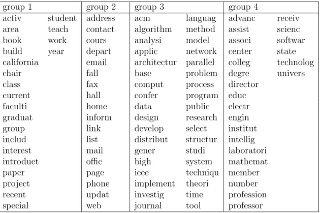
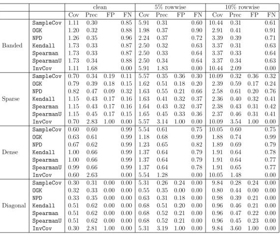
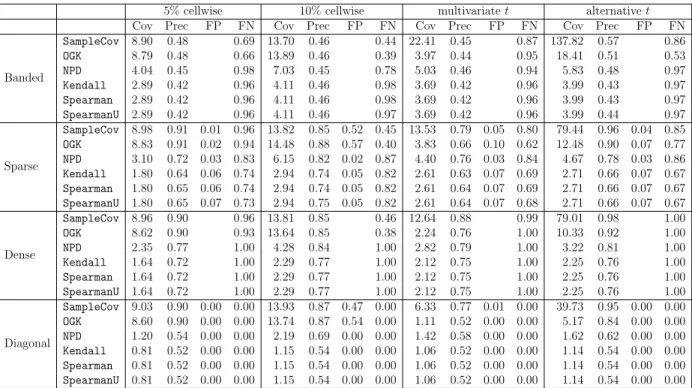
2.1 Keywords in group 1 to group 4. . . 58 3.1 Simulation results for seven estimators and four sampling schemes,

when n = 200 and p= 120. Performance is measured by kΣˆ −Σ∗k∞

for covariance matrix estimation (Cov),kΩˆ−Ω∗k∞for precision matrix

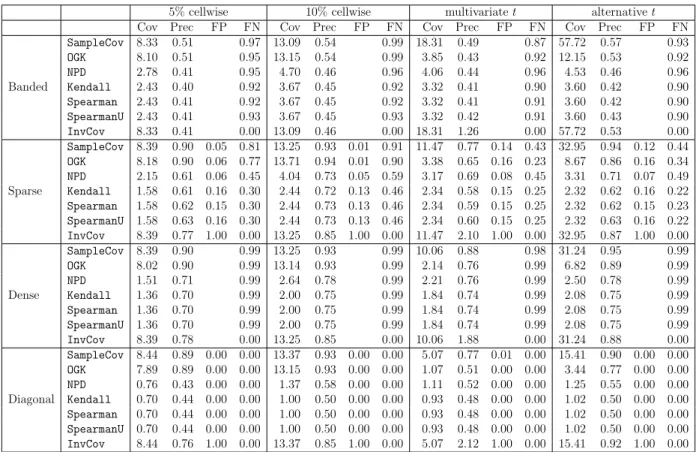
estimation (Prec), and false positive rate (FP) and false negative rate (FN) for support recovery of the true precision matrix. The results are averaged over 100 replications. . . 111 3.2 Simulation results for seven estimators and four sampling schemes,

when n = 200 and p= 120. Performance is measured by kΣˆ −Σ∗k∞

for covariance matrix estimation (Cov),kΩˆ−Ω∗k∞for precision matrix

estimation (Prec), and false positive rate (FP) and false negative rate (FN) for support recovery of the true precision matrix. The results are averaged over 100 replications. . . 112

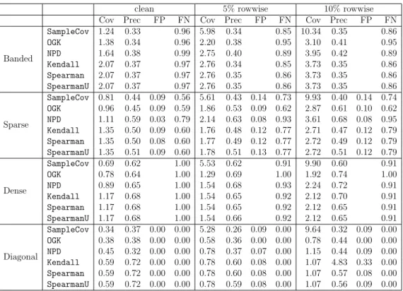
3.3 Simulation results for six estimators and four sampling schemes, when

n = 200 and p = 400. Performance is measured by kΣˆ −Σ∗k∞ for

covariance matrix estimation (Cov), kΩˆ −Ω∗k∞ for precision matrix

estimation (Prec), and false positive rate (FP) and false negative rate (FN) for support recovery of the true precision matrix. The results are averaged over 100 replications. . . 113 3.4 Simulation results for six estimators and four sampling schemes, when

n = 200 and p = 400. Performance is measured by kΣˆ −Σ∗k∞ for

covariance matrix estimation (Cov), kΩˆ −Ω∗k∞ for precision matrix

estimation (Prec), and false positive rate (FP) and false negative rate (FN) for support recovery of the true precision matrix. The results are averaged over 100 replications. . . 114 C.1 Minimax rates of convergence in the sparse regime: 0 < < β₂. . . 215 C.2 Minimax rates of convergence in the moderately dense regime: β₂ ≤

≤ 3β

4 . In this case, we have 2−β

4 ≤

β−

2 . . . 215

C.3 Minimax rates of convergence in the strongly dense regime: 3₄β < ≤β. In this case, we have β−₂ < 2₄−β. . . 215

List of Figures

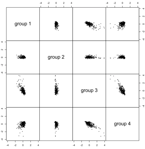
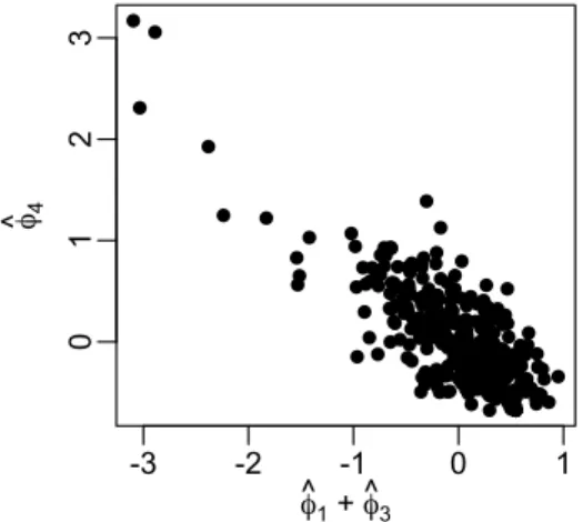
2.1 Pairwise scatterplot of the smallest kernel APC scores for the university webpages data. The eigenvalue for the APC is 0.0910. . . 59 2.2 Plot of ˆφ4 against ˆφ1+ ˆφ3 in the smallest kernel APC for the university

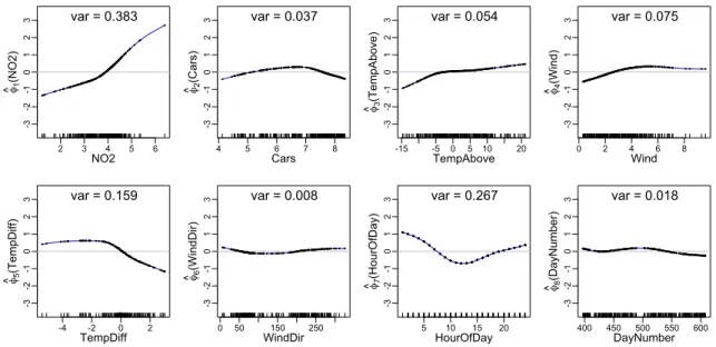
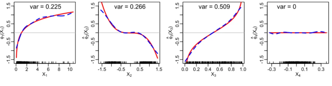
webpages data. . . 60 2.3 The smallest kernel APC transformations for the N O2 data, using

Sobolev kernel of order 2 for each variable. The eigenvalue for the APC is 0.0621. The black bars at the bottom of each panel indicate the location of data points for that variable. . . 63 2.4 The second-smallest kernel APC transformations for the N O2 data,

using Sobolev kernel of order 2 for each variable. The eigenvalue for the APC is 0.0827. The black bars at the bottom of each panel indicate the location of data points for that variable. . . 63 2.5 The third-smallest kernel APC transformations for theN O2 data,

us-ing Sobolev kernel of order 2 for each variable. The eigenvalue for the APC is 0.189. The black bars at the bottom of each panel indicate the location of data points for that variable. . . 64

2.6 Plot of population APC transformations ( ) and sample kernel APC transformations ( ). The eigenvalue for the sample kernel APC is 0.014. The black bars at the bottom of each panel indicate the location of data points for that variable. . . 67 4.1 Plot of the rate exponentr(β, , b) against the signal strengthb. In the

sparse regime ( ),r(β, , b) changes in the order 2+ 8b−2,2+ 4b−

2, +6b−2. In the moderately dense regime ( ),r(β, , b) changes in the order 2+ 8b−2,2−2, β+ 4b−2, + 6b−2. In the strongly dense regime ( ),r(β, , b) changes in the order 2+8b−2,2−2, +6b−2. Top row, left panel: a continuum view of r(β, , b) as increases from 0 to β = 0.45 (color changes from red to blue). Top row, right panel: a static view of each regime: sparse (= 0.12), moderately dense ( = 0.28), and strongly dense (= 0.4). Transition points are indicated by the knots on the dashed lines. Bottom row, left panel: a continuum view ofr(β, , b) asβ increases from= 0.2 to 0.5 (color changes from blue to red). Grey vertical lines indicateb = 0 andb= ₂. Bottom row, right panel: a static view of each regime: strongly dense (β = 0.25), moderately dense (β = 0.35), and sparse (β = 0.45). . . 135 4.2 Plot of MSE for the estimators Qb₀, Qb₂, and Qb₄ over different sample

sizes n ∈ {103, . . . ,107}, in the log-log scale. Fixing β = 0.45, the columns are ordered from left to right as = 0.02 (sparse regime), = 0.3 (moderately dense regime), and = 0.44 (strongly dense regime). The rows are ordered from top to bottom in increasing signal strength:

b∈ {−0.1,0.15,0.2}. Solid line has a slope equal to that of the optimal rate exponentr(β, , b). . . 138

1

Introduction

In the past decades, advances in technology have enabled collection of massive amounts of data, opening the door to a new approach to understanding the world and making decisions. Despite the wealth of data available, the ability to unlock the value in data rests on our ability to summarize the data and provide interpretation of the summary quantities computed. Such summaries and corresponding interpretations can rarely be produced by just looking at the raw data, and a careful scientific scrutiny and statistical analysis are crucial for the generation of valuable insights from data.

Often times, the data collected involves measurements of multiple variables on the same unit, rendering the variables correlated and univariate analyses insufficient for deriving conclusion and guiding next steps. In these cases, a statistical analysis of the dependencies structure of the variables is essential. The study of dependence relations among multiple variables of interest is at the heart of multivariate statistics, and is the focus of this thesis. There are three main chapters within the body of this thesis, each of which is a single, self-contained paper. While the topics studied in these chapters fall under the general realm of multivariate statistics, they also come with interesting twists by having connections to nonlinear statistics, robust statistics, as well as high-dimensional statistics.

Kernel Additive Principal Components

In Chapter 2, we study additive principal components (APCs for short), a nonlinear generalization of linear principal components. We focus on smallest APCs to describe additive nonlinear constraints that are approximately satisfied by the data. Thus, an APC analysis fits data with implicit equations that treat the variables symmetrically, as opposed to regression analyses which fit data with explicit equations that treat the variables asymmetrically by singling out a response.

APCs were initially proposed by Donnell et al. (1994), where a subspace restric-tion regularizarestric-tion approach was introduced for estimating APC transformarestric-tions. In this chapter, we cast APCs in the context of penalized least squares and reproduc-ing kernel Hilbert spaces (RKHSs), and take advantage of the extensions offered by kernelizing. In contrast to the existing subspace restriction approach, kernelizing approaches achieve regularization through shrinkage and therefore grant distinctive flexibility in APCs estimation by allowing the use of infinite-dimensional function spaces while retaining computational feasibility. Furthermore, the interpretation of regularization kernels as similarity measures makes possible the exploration of im-plicit additive redundancies in non-Euclidean data, a flexibility not available in the original APC proposal.

Introducing kernelizing into a multivariate method is not a mechanical exercise. We motivate our formulation of kernel APCs by the Null Comparison Principle, a principle that ties the constraint in a multivariate problem to its criterion in a way that makes the goal of the multivariate method under study transparent. This sim-ple yet powerful princisim-ple is potentially useful for devising generalizations of other multivariate methods and thus can be of independent interest.

On the other hand, kernel canonical correlation analysis (CCA) is a special case of kernel APCs with two variables, and the statistical convergence of kernel CCA was

first established in Fukumizu et al. (2007). In this chapter, we establish the statistical convergence of kernel APCs under a decay rate for regularization parameters involved that is less stringent than that in Fukumizu et al. (2007). Our proof of convergence is built on an elegant RKHS-based theory we develop for APCs, which covers general RKHSs not studied in Fukumizu et al. (2007) and do not require the population targets to lie in RKHSs a priori. Our theory also motivates an iterative algorithm for computing finite-sample kernel APCs. Lastly, we provide data examples, simulated and real, to illustrate the kernel APC methodology. Supplementary materials for this chapter can be found in Appendix A.

This chapter is joint work with Andreas Buja and Zongming Ma.

High-dimensional Robust Precision Matrix

Estima-tion: Cellwise Corruption under

-Contamination

In Chapter 3, we analyze theoretical properties of robust estimators for precision ma-trices, when data are contaminated in a cellwise manner: each element of the data matrix is independently corrupted according to a certain proportion. Such contami-nation mechanisms may be used to model various phenomena in real-world scientific data, including measurement error in DNA microarray analysis and dropouts in sensor arrays.

When data follows an uncontaminated multivariate normal distribution, the graph-ical Lasso (GLasso) (Yuan & Lin, 2007; Banerjee et al., 2008; Friedman et al., 2008) and the constrained `1-minimization for inverse matrix estimation (CLIME) (Cai

et al., 2011) estimators are known to possess rigorous theoretical guarantees for the estimation of precision matrices in high dimensions; however, their performance may be compromised severely when data are contaminated by even a single outlier.

The estimators we study are inspired by techniques in robust statistics and are constructed by plugging appropriately chosen robust covariance matrix estimators into the GLasso and CLIME. We derive high-dimensional error bounds that reveal the interplay between the dimensionality of the problem and the degree of contami-nation permitted in the observed distribution, and also analyze the breakdown point of both estimators. Our results show that although the graphical Lasso and CLIME estimators perform equally well from the point of view of statistical consistency, the breakdown property of the graphical Lasso is superior to that of CLIME. We also dis-cuss implications of our work for gaussian graphical model estimation in the presence of contamination, where the goal is to estimate the support of the graph associated with the clean distribution. Our results apply to arbitrary contaminating distribu-tions and allow for a nonvanishing fraction of cellwise contamination. Finally, we examine the performance of our estimators in comparison to that of other (possibly non-robust) estimators through simulation studies. Supplementary materials for this chapter can be found in Appendix B.

This chapter is joint work with Po-Ling Loh.

Optimal Estimation of A Quadratic Functional

un-der the Gaussian Two-Sequence Model

While Chapters 2 and 3 focus on the analysis ofcovariance structure of multiple vari-ables, Chapter 4 involves an analysis of mean structure of the variables. Specifically, we study in Chapter 4 the problem of optimal estimation of the quadratic functional

Q(µ, θ) = _n1 Pn

i=1µ 2

iθ2i under the gaussian two-sequence model. The mean vectors

µ= (µ1, . . . , µn) and θ = (θ1, . . . , θn) are assumed to be sparse.

es-timation problem is motivated by the problem of simultaneous signal detection in integrative genomics, which, under our simplified framework, is equivalent to the detection of locations i where µi and θi are simultaneously non-zero. We propose

optimal estimators of Q(µ, θ) and establish the minimax rates of convergence over a family of parameter spaces. Interestingly, the optimal rates exhibit different phase transitions in three regimes, each characterized by the sparsity of simultaneous non-zero means relative to that of non-non-zero entries in individual mean vectors. Along with the establishment of the minimax rates of convergence, we explain the intuition behind the construction of the optimal estimators in each regime. A simulation study is included to complement the theoretical results in the chapter. We also give a brief discussion on the application of quadratic functional estimators to the problem of si-multaneous signal detection. Supplementary materials for this chapter can be found in Appendix C.

2

Kernel Additive Principal Components

2.1

Introduction

Linear principal component analysis (PCA) is a tool commonly used to reduce the dimensionality of data sets consisting of several interrelated variablesX1, X2, . . . , Xp.

PCA amounts to finding linear functions of the variables, P

ajXj, whose variances

are maximal or, more generally, large and stationary under a unit norm constraint,

P

a2_j = 1. These linear combinations, called largest linear principal components

(largest LPCs for short), are thought to represent low-dimensional linear structure of the data. The reader is referred to Jolliffe (2002) for a comprehensive review of PCA. One can similarly define the smallest linear principal component (smallest LPCs) as linear functions of the variables whose variances are minimal or small and sta-tionary subject to a unit norm constraint on the coefficients. If these variances are near zero, Var (P

ajXj)≈ 0, the interpretation is that the data lie near the

hyper-plane defined by the linear constraint P

ajXj = 0 (assuming that the variables Xj

are centered). Thus the purpose of performing PCA on the lower end of the

pal components spectrum is quite different from that of performing it on the upper end: largest principal components are concerned with structure of low dimension, whereas smallest principal components are concerned with structure of low codimen-sion. Largest LPCs provide projections to low dimensions, whereas smallest LPCs provideimplicit equations to approximate linear dependencies among variables.

The topic of this chapter is a generalization of smallest linear principal compo-nents in function spaces, called “smallest additive principal compocompo-nents” (“APCs” for short). APCs were initially proposed by Donnell et al. (1994) before kernelizing became a well-understood methodology. The goal of this chapter is to cast APCs in the context of penalized least squares and reproducing kernel Hilbert spaces (RKHSs), and take advantage of the extensions offered by kernelizing.

Before proceeding, here is a brief summary of additive approaches to multivariate function fitting: The step from a linear method to an additive method consists of replacing linear terms ajXj with nonlinear terms φj(Xj), thereby allowing nonlinear

marginal transformations of the coordinate variables Xj, each to be estimated by

some nonlinear fitting method. It is known that additive approaches avoid the curse of dimensionality that fully nonlinear function fitting φ(X1, X2, ..., Xp) would entail.

Historically the generalization from linear to additive approaches first appeared in the context of regression, where fitting linear equations Y ∼ P

jajXj was extended to

fitting additive equationsY ∼P

jφj(Xj) to a responseY, as documented by Breiman

& Friedman (1985), Buja et al. (1989), culminating in the classical book by Hastie & Tibshirani (1990). Additive extensions were enabled at the time by the emergence of fast smoothing technology that allows estimation and computation of suitably regularized transformations φj(Xj) with an iterative algorithm called “backfitting”,

whereby each φj(Xj) is updated in turn by a smoothing step of partial residuals on

Xj: Y−

P

Xj, that reveal the nonlinearities graphically, while relative variable importances are

measured by the standard deviations of the transforms φj(Xj).

Similar to the additive extension of linear regression, the additive extension of LPCs implies the replacement of the linear terms ajXj with nonlinear termsφj(Xj),

hence an additive principal component is of the formP

φj(Xj). In additive regression

it is approximation of the response variable that produces non-trivial transformations; in additive principal components it is a normalizing constraint resulting in an eigen-value problem that achieves the same. In generalizing LPCs to APCs, one therefore needs to find a suitable way to generalize the LPC constraintP

a2

j = 1. Donnell et al.

(1994) proposed to use the constraintP

Varφj(Xj) = 1, their justification being that

forφj(Xj) = ajXj we have Var (φj(Xj)) =a2j for real-valuedXjwith Var (Xj) = 1,

re-sulting in the conventional constraintP

a2

j = 1. Asmallest APC can then be defined

as ap-tuple of marginal transformationsφ1,φ2, . . . ,φp that minimizes Var (

P

φj(Xj))

subject to P

Var (φj(Xj)) = 1.

The interpretation of a smallest APC is that the additive constraint represented by the implicit additive equationP

φj(Xj) = 0 defines a nonlinear or, more precisely,

an additive manifold that approximates the data. Smallest APCs can have multiple methodological uses:

• APCs can be used as a generalized collinearity diagnostic for additive regression models. Just as approximate collinearities P

αjXj ≈0 destabilize inference in

linear regression Y ∼ P

βjXj, additive approximate “concurvities” (Donnell

et al., 1994) of the formP

φj(Xj)≈0 destabilize inference in additive regression

Y ∼ P

ψj(Xj). Such concurvities can be found by applying APC analysis to

the predictors of an additive regression.

desirable to single out any one of the variables as a response. Additive implicit equations estimated with APCs will then freely identify the variables that have strong additive associations with each other.

• Even when there is a specific response variable of interest in the context of an additive regression, an APC analysis of all variables, including predictors as well as response, can serve as an indicator of the strength of the regression, depending on whether the response variable has a strong presence in the smallest APC. If the response shows up only weakly, it follows that the predictors have stronger additive associations among each other than with the response. Examples of applications of smallest APCs will be given in Section 2.9, and simulation examples in Section 2.10.

Estimation of APCs and their transforms φj(Xj) from finite data requires some

form of regularization. There exist two broad classes of regularization in nonparamet-ric function estimation, namely, subspace regularization and shrinkage regularization. Subspace regularization restricts the function estimates ˆφj to finite-dimensional

func-tion spaces on Xj. Shrinkage regularization produces function estimates by adding a

penalty to the goodness-of-fit measure in order to impose the spatial structure of Xj

on ˆφj. Commonly used are generalized ridge-type quadratic penalties (also called the

“kernelizing approach”) and lasso-type `1-penalties. The original APC proposal in

Donnell et al. (1994) only uses subspace regularization for estimation, and it does not provide asymptotic theory for it. In the present chapter we investigate APCs based on shrinkage/kernelizing regularization and provide some asymptotic consistency theory. It should be pointed out that introducing a shrinkage/kernelizing approach into a multivariate method is not a mechanical exercise. It is not a priori clear where and how the penalties should be inserted into a criterion of multivariate analysis, which in the case of PCA is variance subject to a constraint. The situation differs from

regression where there is no conceptual difficulty in adding a regularization penalty to a goodness-of-fit measure. In a PCA-like method such as APC analysis, however, it is not clear whether penalties should be added to, or subtracted from, the variance, or somehow added to the constraint, or both. An interesting and related situation occurred in functional multivariate analysis where the same author (B. Silverman) co-authored two different approaches to the same PCA regularization problem (Rice & Silverman, 1991; Silverman, 1996), differing in where and how the penalty is inserted. Our approach, if transposed to functional multivariate analysis, agrees with neither of them. One reason for our third way is that neither of the approaches in Rice & Silverman (1991) or Silverman (1996) generalize to the low end of the PCA spectrum. In contrast, the regularized criterion proposed in this chapter can be applied to the high and the low end of the spectrum, and hence to the discovery of low dimension as well as low co-dimension. Our more specific interest is in the latter.

An immediate benefit of injecting penalty regularization into multivariate anal-ysis stems from recent methodological innovations in kernelizing. These include the possibility of using infinite-dimensional function spaces, the interpretation of regular-ization kernels as positive definite similarity measures, and the kernel algebra with the freedom of modeling it engenders. Two decades ago, when Donnell et al. (1994) was written, it would have been harder to make the case for penalty regularization.

In what follows we first describe the mathematical structure of APCs and give a review on population APCs that constitute our targets of estimation (Section 2.2). Section 2.3 introduces the Null Comparison Principle that guides the derivation of our kernel APC problem in Section 2.4. Section 2.5 poses the kernel APC problem in the framework of reproducing kernel Hilbert spaces. Although our focus on the lower end of the spectrum seems to have found little precedence in the literature, the criterion we use for kernel APC turns out to be equivalent to that of kernel canonical

correlation analysis (kernel CCA) (Bach & Jordan, 2003), a nonlinear extension of canonical correlation analysis, when there are only two variables of interest. The statistical convergence of kernel CCA was first established in Fukumizu et al. (2007). In Section 2.6, we establish the statistical convergence of kernel APCs under a decay rate for regularization parameters involved that is less stringent than that in Fuku-mizu et al. (2007). Our proof of convergence is built on an elegant RKHS-based theory we develop for APCs in Section 2.5, which covers general RKHSs not studied in Fukumizu et al. (2007) and do not require the population targets to lie in RKHSs a priori. Section 2.7 presents the power algorithm for computing kernel APCs, whereas Section 2.8 contains a brief discussion on the selection of penalty parameters. In Section 2.9 we present the kernel APC methodology in terms of two data examples. Section 2.10 contains simulation studies to complement our theoretical results. A discussion on the relation of kernel APC with kernel PCA (Sch¨olkopf et al., 1998; Sch¨olkopf & Smola, 2002) and kernel CCA is given in Section 2.11. Section 2.12 con-cludes. To deal with the generality of RKHSs considered in Section 2.5, we need some technical results whose proofs are collected in Appendix A.1. Proofs of the consis-tency results stated in Section 2.6 are given in Appendix A.2, whereas proofs related to the power algorithm of Section 2.7 are given in Appendix A.3. Appendix A.4 con-tains implementation details for the power algorithm, while Appendix A.5 concon-tains an alternative linear algebra method for computing sample kernel APCs. Details on the comparison of kernel APC with kernel PCA is given in Appendix A.6.

The following notations and concepts in functional analysis are useful for the discussion that follows.

Notation: LetH,H1,H2 be Hilbert spaces. In this chapter, a Hilbert space always

means a separable Hilbert space. We denote the norm of a bounded linear operator

are denoted by N(T) and R(T), respectively, where N(T) = {φ ∈ H1 : Tφ = 0}

and R(T) = {Tφ ∈ H2 : φ ∈ H1}. We denote by T∗ the Hilbert space adjoint of

T. We say that T : H → H is self-adjoint if T∗ = T, and that a bounded linear self-adjoint operator T is positive if hφ,Tφi ≥ 0 for all φ∈ H. We write T0 if T

is positive, andT1 T2 ifT1−T2 is positive. IfTis positive, we denote byT1/2 the

unique positive operator B satisfying B2 =T. On the other hand, a bounded linear operator T : H1 → H2 is compact if T takes bounded sets in H1 into precompact

sets in H2. One nice property of a compact operator is the availability of singular

value decomposition: for some N ∈_N∪ {∞}, there exist (not necessarily complete) orthonormal sets{φν}Nν=1 ⊂ H1 and{ψν}Nν=1 ⊂ H2 and positive real numbers{λν}Nν=1

called singular values, such that

T=

N

X

ν=1

λνhφν,·iH1ψν.

If N = ∞, then λν → 0 and the infinite series in the equation above converges in

norm. We say that a bounded linear operator T : H1 → H2 is Hilbert-Schmidt

if P∞ k=1 P∞ l=1hψl,Tφki 2 H2 = P∞ k=1kTφkk 2

H2 < ∞ for a complete orthonormal basis

system (CONS) {φk}∞k=1 of H1 and {ψl}∞l=1 of H2. It is known that this sum is

independent of the choices of CONS. For two Hilbert-Schmidt operators T1 and T2,

the Hilbert-Schmidt inner product is defined by

hT1,T2iHS= ∞ X k=1 ∞ X l=1 hψl,T1φkiH2hψl,T2φkiH2 = ∞ X k=1 hT1φk,T2φkiH2,

with which the set of all Hilbert-Schmidt operators from H1 to H2 form a Hilbert

space. The Hilbert-Schmidt norm kTkHS is again given by kTk2HS = hT,TiHS =

P∞

k=1kTφkk2H2. Obviously, ifT is Hilbert-Schmidt, then kTk ≤ kTkHS. Moreover, a

iff the singular values satisfy P

λ2

ν < ∞. For other standard functional analysis

concepts, see Reed & Simon (1980).

2.2

Population APCs

In this section, we give a review on population APCs (Donnell et al., 1994) which forms the foundation for RKHS-based theory of APCs in later sections.

2.2.1

Transformations and Their Interpretations

Let X1, . . . , Xp be random variables taking on values in arbitrary measurable spaces

(X1,BX1), . . ., (Xp,BXp), each of which can be continuous or discrete, temporal or

spatial, high- or low-dimensional. The only assumption at this point is that they have a joint distribution P1:p(dx1, . . . , dxp) on X1 × · · · × Xp. Quantitative random

variables φj(Xj) can be obtained by applying real-valued functions φj : Xj → IR to

the arbitrarily-valued Xj. The functions φj are often interpreted as “scorings” or

“scalings” or “quantifications” of the underlying spaces Xj. If Xj is already

real-valued, then φj is interpreted as a variable transformation.

Donnell et al. (1994) considers functions φj that belong to some closed subspace

Hj of square-integrable functions with regard to their marginal distributionsPj(dxj):

φj ∈Hj ⊂L2(Xj, Pj) :={φj :E(φ2j(Xj))<∞}.

The role of the coefficient vectora= (a1, . . . , ap)T in LPCs is taken on by a vector of

transformations:

Similarly, the role of the linear combination P

ajXj in LPCs is taken on by an

additive function P

φj(Xj). APCs contain LPCs as a special case when all Xj are

real-valued with unit variances and Hj = {φj : φj(xj) = ajxj, aj ∈ IR}. A smallest

APC (associated with H) is now defined as a solution to

min Φ∈HVar ( p X j=1 φj(Xj)) subject to p X j=1 Var (φj(Xj)) = 1. (2.2) When H = L2_(X

1, P1)× · · · ×L2(Xp, Pp), a solution to (2.2), if it exists, is said to

be a population APC. We will use population APCs as targets of estimation, and in this we differ, for example, from Fukumizu et al. (2007) who assume their targets of estimation to be in RKHSs. In the present work, the role of RKHS theory is to provide regularization devices for estimation, but the targets of estimation may fall outside and will be reached in the limit in the L2 _{sense. RKHS theory appropriate}

for APCs is the subject of Sections 2.4−2.6.

2.2.2

A Note on the Role of Constants

A particular nuisance in the context of APCs is the non-identifiability of constants in additive functions P

φj. For example, ˜φk =φk+c, ˜φl =φl−c for some k 6=l (and

˜

φj =φj else) result in the same additive function,

P˜

φj =

P

φj. Donnell et al. (1994)

deal with this issue by takingHj to be closed subspaces of centered transformations,

Hj = L2c(Xj, Pj) := {φj : E(φj(Xj)) = 0, E(φ2j(Xj)) < ∞}. This approach raises

unnecessary questions because strictly speaking estimates ˆφj of the transformations

φj cannot be centered at the population mean (which is not known) and hence cannot

be inHj. Yet it is obvious that this should a non-issue if viewed appropriately.

Our preferred solution is to considerL2_(X

j, Pj) as consisting of equivalence classes

con-stant. This may be expressed as L2_(X

j, Pj)/IR, but for notational simplicity we

continue writing L2_(X

j, Pj) with the understanding that its elements are intended

modulo constants. It is then straightforward to check that L2_(X

j, Pj) is a Hilbert

space wrt covariance as the inner product:

hφj, ψjiPj := Cov(φj(Xj), ψj(Xj)), (2.3)

where φj and ψj are any functions in their respective equivalence classes modulo

constants. Our framework therefore says that differences by constants are irrelevant and should be ignored. We will have to make sure that quantities of interest defined onL2(Xj, Pj) are invariant under φj 7→φj +cj.

2.2.3

Population APCs — Review

We adapt a few facts about population APCs from Donnell et al. (1994) which prefig-ure some of the steps that will be required for RKHS-based theory of APCs. The first fact is the reformulation of APCs in terms of function spaces and operators between them. The second fact is the existence of APC solutions under suitable assumptions, here chosen a little stronger than in Donnell et al. (1994), namely, the Hilbert-Schmidt property rather than compactness of operators. The operator representation was in-spired by a natural power algorithm (Section 2.7) which in turn was inin-spired by the ACE algorithm of Breiman & Friedman (1985).

We first introduce the natural inner product and associated norm for p-tuples of functions, Φ,Ψ ∈ H∗ := L2(X1, P1)× · · · × L2(Xp, Pp), turning H∗ into a Hilbert

space: hΦ,ΨiP := p X j=1 hφj, ψjiPj = p X j=1 Cov(φj(Xj), ψj(Xj)),

kΦk2_P := p X j=1 kφjk2Pj = p X j=1 Var (φj(Xj)).

The APC constraint can now be expressed bykΦk2

P = 1. To do likewise for the APC

criterion, we introduce operators to express

Var (P jφj(Xj)) = P jVar (φj(Xj)) + P i,jCov(φi(Xi), φj(Xj))

in terms of inner products h·,·iPi. Let ψi(Xi) = E(φj(Xj)|Xi). We note that

Cov(φi(Xi), φj(Xj)) = Cov(φi(Xi), E(φj(Xj)|Xi)) = hφi, ψiiPi.

Thus the required operators are the conditional expectations between theL2 spaces:

Pij :L2(Xj, Pj)→L2(Xi, Pi), φj 7→Pijφj = ψi.

These are also the orthogonal projections between the respective subspaces: Pijφj =

argmin_f∈L2_(X

i,Pi)Var (φj(Xj)−f(Xi)) (leaving constants undetermined; see Section 2.2.2.)

Finally, we collect the operators Pij in a matrix to act as an operator on H∗:

P= (Pij)i,j, where the ith component mapping is given by

(PΦ)i :=

P

jPijφj ∈L

2_(X

i, Pi). (2.4)

Thus the population APC problem can be stated as

minΦ∈H∗hΦ,PΦi_P subject to kΦk2_P = 1. (2.5)

The existence of solutions to (2.5) can be granted under certain conditions. We are not striving for generality but for simplicity, hence we adopt the technically con-venient condition that the conditional expectation operators Pij (i 6=j) have the

Hilbert-Schmidt property. Assuming that the spaces L2_(X

i, Pi) and L2(Xj, Pj) are

separable and hence have countable orthonormal bases (φik)k and (φjl)l, the

Hilbert-Schmidt property can be stated as the following requirement, which can be shown to be independent of the particular bases:

kPijk2HS := P

k,lhφik, Pijφjli

2

Pi < ∞.

Such Hilbert-Schmidt operators form a Hilbert space with k · kHS as the norm. For

Pij the property amounts to a condition on the covariance functional onL2(Xi, Pi)×

L2_(X j, Pj): kPijk2HS = P k,l Cov(φik(Xi), φjl(Xj) ) 2 _{< ∞,}

which is equivalent to the following condition on the joint distribution:

Z Z _p2 Xi,Xj(xi, xj) pXi(xi)pXj(xj) dxidxj = EPi⊗Pj p2_Xi,Xj(xi, xj) p2 Xi(xi)p 2 Xj(xj) ! < ∞.

The Hilbert-Schmidt property limits the strength of the association between Xi

and Xj by limiting how far the actual joint distribution pXi,Xj(xi, xj) can be from

independence, pXi(xi)pXj(xj). It precludes, for example, X1 = · · · = Xp. See Buja

(1990) for context.

To calculate the Hilbert-Schmidt norm for operator matrices such asP, we embed the bases (φjl)l of L2(Xj, Pj) in H∗ through φjl 7→ Φj,l = (0, . . . ,0, φjl,0, . . . ,0)0, so

(Φj,l)j,l forms an orthonormal basis of H∗. Now, the Hilbert-Schmidt norm of P is

infinite becausePjj =IdL2_(X

are Hilbert-Schmidt: kP−IdH∗k2 HS= X i6=j;k,l hΦi,k,PΦj,li2P = X i6=j X k,l hφik,Pijφjli2Pi =X i6=j kPijk2HS < ∞.

BecauseP−IdH∗ is Hilbert-Schmidt and self-adjoint wrth·,·i_P (Donnell et al. (1994),

Lemma 4.1), it has an eigen expansion:

(P−IdH∗)Φ = P ν λ 0 νhΦ,ΦνiP Φν, P νλ 02 ν = kP−IdH∗k2_HS < ∞,

where (Φν)ν form a complete orthonormal system of eigenvectors for P−IdH∗, and

(λ0_ν)ν is the set of corresponding eigenvalues with 0 as the only possible accumulation

point. This translates to an eigen expansion of P:

λν :=λ0ν + 1 ⇒ PΦ =

P

ν λνhΦ,ΦνiP Φν,

P

ν(λν−1)2 <∞. (2.6)

It can be shown that 0 ≤ λν ≤ p (Donnell et al., 1994). Since the only possible

accumulation points of λν is +1, we will use +1 as a natural dividing lines between

small and large APCs. To relate the expansion (2.6) back to the population APC problem (2.5), form the inner product with Φassuming unit norm:

kΦk2 P = 1 ⇒ hΦ,PΦiP = P_ν λνhΦ,Φνi2P and P νhΦ,Φνi 2 P = 1. (2.7)

From (2.7) follows that the APC minimization problem (2.5) has the following solu-tion:

minkΦk2

Any eigenvector Φν with minimizing eigenalue λν is therefore a smallest population

APC.

For an understanding of APCs, it is important to know the situation in which APCs are unable to discover association among variables. The following equivalent statements from Donnell et al. (1994), Proposition 4.8, characterize the “null situa-tion” for APCs:

minνλν = 1 ⇔ maxνλν = 1 ⇔ λν = 1 ∀ν ⇔ Pij =0 ∀i6=j

⇔ L2_(X

i, Pi)⊥L2(Xj, Pj) ∀i6=j ⇔ Xi, Xj independent ∀i6=j

Pairwise independence is not the same as full independence. Thus APCs can only find association that is detectable through pairwise association, which is natural because APCs rely on covariances Cov(φi(Xi), φj(Xj)). This, however, should be a “limited

limitation” as in practice multivariate associations are unlikely to hide behind pairwise independence.

2.3

Criterion and Constraint — A Null

Compari-son Principle

Donnell et al. (1994) chose the constraint P

Var (φj) = 1 for APCs because it

gener-alizes the contraint of LPCs. Generalization is a convenient justification but, as will be seen, it is insufficient to guide us in kernelizing APCs. Without a guiding princi-ple, attempts at kernelizing multivariate methods end up relying on ad hoc proposals, some of which we discuss in Section 2.4.2. Even for LPCs we may ask: what is it that makes P

a2_j = 1 “natural” as a constraint? When variables are heterogeneous with incompatible units, one tends to standardize the variables before using the constraint

P

a2

j = 1. This, on the other hand, is equivalent to using

P

a2

jVar (Xj) = 1 as

the constraint on the unstandardized variables. Thus practioners have been aware of issues surrounding the constraint since the inception of LPCs. Constraints seem like separate choices, detached from the criteria. To show that this is not so and that there exists a tight coupling between criteria and constraints, we introduce the following:

Null Comparison Principle for multivariate analysis: The quadratic form to be used for the constraint is the optimization criterion evaluated under the null assumption of vanishing correlations of interest.

Here are a number of illustrations of the principle, three for extant linear multivariate methods, and three for their additive analogs.

• For LPCs the criterion is Var (P

ajXj), and the null assumption of interest is

Cov(Xj, Xk) = 0 ∀j 6=k.

The evaluation of the criterion under the null assumption results in

Var (P

ajXj) = PVar (ajXj) = Pa2jVar (Xj),

which evaluates to the familiarP

a2_j if the variables are standardized.

• For Canonical Correlation Analysis (CCA), one divides the variables into two blocks, X1, . . . , Xp and Y1, . . . , Yq. The criterion is still the variance of a linear

combination of all variables: Var (P

aiXi+

P

bjYj). The correlations of interest

Under this “null assumption” the criterion evaluates to Var (P

aiXi)+Var (PbjYj).

Thus the CCA problem is seen to be

maxai,bj Var ( P aiXi+ P bjYj) subject to Var ( P aiXi) + Var ( P bjYj) = 1,

which is algebraically equivalent to the more familiar form

maxai,bj Cov( P aiXi, P bjYj) subject to Var ( P aiXi) = Var ( P bjYj) = 1.

• Multi-block versions called “Generalized Canonical Analysis” (GCA) can be obtained by expanding from two to three or more blocks. Here is for three blocks of variables, X1, . . . , Xp, Y1, . . . , Yq and Z1, . . . , Zr: The criterion is

Var (P

aiXi +PbjYj +PckZk), and the null assumtion is vanishing

corre-lations between the blocks, that is,

Cov(Xi, Yj) = Cov(Xi, Zk) = Cov(Yj, Zk) = 0 ∀i, j, k.

Under this null assumption the criterion evaluates in the familiar way, and the three-block GCA problem can be stated as

maxai,bj,ck Var ( P aiXi+ P bjYj + P ckZk) subject to Var (P aiXi) + Var (PbjYj) + Var (PckZk) = 1.

LPC is then GCA withp blocks and every block containing only one variable.

• Turning from linear to additive methods, for APCs the criterion is Var (P

and the null assumption of interest is

Cov(φi(Xi), φj(Xj)) = 0 ∀φi, φj, i6=j. (2.9)

The evaluation of the criterion results in Var (P

φj(Xj)) = PVar (φj(Xj)),

hence the null comparison principle leads to the familiar form of the APC prob-lem: minφj Var ( P φj(Xj)) subject to P Var (φj(Xj)) = 1.

• To further illustrate the null comparison principle we show how additive CCA can be devised, without further pursuing it later on: Again, the variables are divided into two blocks as in linear CCA, but the criterion is Var (P

φi(Xi) +

P

ψj(Yj)). The null assumption is

Cov(φi(Xi), ψj(Yj)) = 0 ∀φi, ψj

The evaluation of the criterion under the null assumption leads to the following:

maxφi,ψj Var ( P φi(Xi) + P ψj(Yj)) subject to Var (P φi(Xi)) + Var ( P ψj(Yj)) = 1.

When the Y-block contains just one variable, additive CCA amounts to the ACE method of Breiman & Friedman (1985).

• It is now obvious how a multi-block version of additive GCA can be devised, and we may simply skip to its final form for three blocks:

maxφi,ψj,ξk Var ( P φi(Xi) + P ψj(Yj) + P ξk(Zk)) subject to

Var (P

φi(Xi)) + Var (Pψj(Yj)) + Var (Pξk(Zk)) = 1.

Again, APC amounts to additive GCA withp blocks, each block with just one variable.

These examples illustrate how the null comparison principle ties the constraint to the criterion, thereby making it less an arbitrary choice. The choice is no longer that of a constraint but of a null assumption that identifies the correlations of interest and assumes them to vanish. The constraint is then derived by evaluating the criterion under the null assumption. We thus arrive at a powerful and principled way of devising generalizations of multivariate methods, a way whose real power will be revealed when we introduce penalized APCs.

2.4

Penalized APCs

In this section, we derive the penalized APC problem using the null comparison prin-ciple introduced previously. We also give a brief discussion on alternative approaches to penalizing APCs.

2.4.1

Introducing Penalties in APCs Using the Null

Com-parison Principle

Estimation of APCs from finite data requires some form of regularization. The estima-tion procedure of Donnell et al. (1994) can be characterized as using finite-dimensional subspacesHj (possibly adapted to the data, as for regression splines with knots placed

at empirical quantiles) and replacing the population distribution with the empirical distribution of the data. Regularization necessary for estimation is achieved by choos-ing a suitably low dimensionality of the spaces Hj.

In this chapter we will consider APC estimation based on kernelizing whereby regularization is achieved through additive quadratic penaltiesJj(φj) that are scaled

versions of (squared) semi-norms derived from reproducing kernels. While estimation is again based on the empirical distribution, a regularized population version based on the actual distributionP1:p exists also and is useful for bias-variance calculations.

For simplicity of notation we continue the discussion using the population case. The natural optimization criterion for kernel APCs is penalized variance:

Var ( p X j=1 φj) + p X j=1 Jj(φj). (2.10)

This choice forces the transformations φj not only to generate small variance but

also regularity in the sense of the penalties. A concrete example is the cubic spline penalty Jj(φj) =αj

R

(φ00_j(xj))2dxj for a quantitative variableXj (where we absorbed

the tuning constant αj inJj), but the reader versed in kernelizing will recognize the

generality of modeling offered by penalties derived from general reproducing kernels. The question is next what the natural constraint should be. Informed by the null comparison principle of Section 2.3, we will not naively carry P

Var (φj) = 1 over to

the kernelized problem. Instead we evaluate the criterion (2.10) under the assumption of absent correlations between the transformationsφj, resulting in

p X j=1 Var (φj) + p X j=1 Jj(φj) = 1. (2.11)

As it turns out, this formulation produces meaningful results both for minimization

and maximization. It therefore serves both for estimating smallest APCs, hence im-plicit additive equations (structure of low co-dimension), and for estimating largest APCs, hence additive dimension reduction (structure of low dimension). In the present chapter we pursue the former goal, but we take the well-posedness of both

the minimization and maximization problems as evidence that the approach based on the null comparison principle is sound. As is shown in Sections 2.4.2 and 2.11.1, some generalizations of PCA are not sound in this regard, one of them being kernel PCA.

On data we will replace the population quantities in equations (2.10) and (2.11) with their sample counterparts. As is usual, the penalties will be expressed in terms of quadratic forms of certain kernel matrices.

2.4.2

Alternative Approaches to Penalized APCs

A brief historic digression is useful to indicate the conceptual problem solved by the null comparison principle: As mentioned in the introduction, in the related but dif-ferent field of functional multivariate analysis, Silverman co-authored two difdif-ferent approaches to the same PCA regularization problem where largest principal com-ponents are sought for dimension reduction. These can be transposed to the APC problems as follows: max φj Var (Xφj)− X Jj(φj) subject to X Var (φj) = 1, (2.12) max φj Var (Xφj) subject to X Var (φj) + X Jj(φj) = 1, (2.13)

where (2.12) is due to Rice & Silverman (1991) and (2.13) is due to Silverman (1996). The first approach (2.12) subtracts the penalty from the criterion, which does what it should do for regularized variancemaximization. It is unsatisfactory for reasons of mathematical aesthetics: a difference of two quadratic forms can result in negative values, which may not be a practical problem but “does not seem right”. The second approach (2.13) solves this issue by adding a penalty to the constraint rather than subtracting it from the criterion, which again does what it should do for variance

maximization. Both approaches can be criticized for resulting in non-sense when the goal is regularized variance minimization. Here the first approach (2.12) is more satisfying because it is immediately clear how to modify it to work for regularized variance minimization: min φ1,...,φp Var (Xφj) + X Jj(φj) subject to X Var (φj) = 1,

whereas for the approach (2.13) it is not clear how it could be modified to work in this case. Subtracting the penalty from the constraint variance, P

Var (φj)−

P

Jj(φj) =

1, is clearly not going to work.

Eschewing these problems, we propose the following kernel APC problem:

min φ1,...,φp Var (Xφj) + X Jj(φj) subject to X Var (φj) + X Jj(φj) = 1. (2.14) The merits of this proposal are that (1) it has no aesthetic issues, (2) it works for both ends of the variance spectrum, and (3) it derives from a more fundamental principle rather than a mathematical ad hoc choice.

2.5

Penalized APCs in Reproducing Kernel Hilbert

Spaces

A preliminary note on vocabulary: Because there will be many occasions to use the clumsy term “squared norm”, we will simplify by using sloppy language whereby the term “norm” stands for both “norm” and “squared norm” according to the context. In this section, we introduce suitable RKHSs for APCs, one per variable. We then formalize the statement of the kernel APC problem (2.14) and establish the existence of solutions. The complications addressed in this section have to do with

the frequent occurrence of penalties that are not norms but semi-norms, such as the cubic spline penalty J(φ) = αR

φ00(x)2_{dx. The relevant quadratic form needed for}

APC constraints, however, is Var (φ) +J(φ). In Section 2.5.1, we establish conditions under which Var (φ)+J(φ) is an RKHS norm. These conditions would be unnecessary if interest were limited to penalties that are actual RKHS norms, but the practical importance of penalties that are semi-norms mandates the mundane elaborations of the present section.

2.5.1

RKHS for APC Variables

Let X be a non-empty set, and let H be a Hilbert space of functions φ : X → IR, endowed with the inner product h·,·iH. The space H is a (real-valued) reproducing kernel Hilbert space if all evaluation functionals (the maps δx : f 7→ f(x), where

x∈ X) are bounded. Equivalently,His an RKHS if there exists a symmetric function

k: X × X → IR that satisfies (a) ∀x ∈ X, kx = k(x,·) ∈ H, (b) the reproducing

property: ∀x∈ X,∀f ∈ H,hf, kxiH=f(x). Such a k is called thereproducing kernel

ofH. There is a one-to-one correspondence between an RKHSH and its reproducing kernel k. Thus, specifying k is equivalent to specifying H, and we may write h·,·ik

for h·,·iH and k · kk fork · kH. Also, kkxk2k =k(x, x).

In principle, regularization through kernelizing can be achieved by taking J(φ) =

αkφk2

k after having specified a kernel (and hence, the corresponding RKHS H). On

the other hand, textbook examples of RKHS include those based on Sobolev type norms such as kφk2

k = φ(a)2 +φ

0_(a)2 ₊R

φ00(x)2_{dx (a∈IR fixed). A pecularity here}

is that the finite-rank part of the norm, φ(a)2 _+φ0_(a)2_{, is arbitrary and not used for}

penalization; only the infinite-rank part is: J(φ) = αR φ00(x)2_{dx, which is the cubic}

spline penalty. Characteristically, this penalty alone is not an RKHS norm, only a semi-norm. To accommodate this situation we introduce the following definitions:

Definitions: Let kφk2

1 = J(φ) on H be a non-negative semi-definite quadratic form

derived from a bilinear form h·,·i1 defined on a function space H, and let

H0 _{:= {φ∈ H | kφk} 1 = 0}

be its null space. We say k · k2

1 is a kernel semi-normif there exists a complement

H1 _{⊂ H of H}0 _{that is an RKHS with regard to the restriction of k · k}2

1 to H1. We call

H1 _{an RKHS complement for k · k}2 1.

We now combine the RKHS structure for regularization with the distributional structure of the data, focusing still on one variable. Consider a measurable space (X,BX) and a random variable X with values inX and distributionP(dx) on X. We

assume a spaceHof functions that areBX-measurable, with a kernel semi-normk · k1

with RKHS complement H1 _{⊂ H. The structure that expresses kernelized APCs is}

given by a combination of the L2_{(X, P) inner product and the RKHS inner product}

based on the penalty kernel k1_:

hφ, ψiα = Cov(φ, ψ) +αhφ, ψi1, kφk2α = Var (φ) +αkφk

2

1 (α >0), (2.15)

where of course Cov(φ, ψ) is understood to mean Cov(φ(X), ψ(X)). To avoid con-fusion in notation, we denote the alpha inner product and norm for the special case

α = 1 by hφ, ψi? and kφk2?, respectively. For (2.15) to represent an RKHS we will

make the following more restrictive assumptions, which, however, suffice to cover the case of Sobolev semi-norms:

Lemma 1. On the linear space H ⊂L2_{(X, P}

X), let kφk21 be a kernel semi-norm with

null space H0 _{and RKHS complementH}1_{. Suppose that H}0 _{is finite-dimensional and}

∞. Then the alpha inner products and norms of (2.15) turnH into an RKHS.

A concern left over by the lemma is that the construction of the RKHS structure on H depends on the specific choice of the space H1_{. While the null space H}0

is unique, the complement H1 _{is not, as evidenced again by the example of cubic}

splines: H1 _{can be defined by a host of different conditions, such as φ(a) =φ}0_{(a) = 0}

for an arbitrary location a, or φ(a) = φ(b) = 0 for two arbitrary locations a < b, or

Rb

a φ(x)dx = 0 and φ(a) = φ(b) again for two arbitrary locations a < b. Different

choices of a and a < b result in different spaces H1_{. Now the question is how two}

different RKHS complements H1 _{and ˜H}1 _{for the same kernel semi-norm somehow}

affect the construction of kφk2

α. It is evident that the choice ofH1 does not affect the

construction as such:

Lemma 2. Let k · k1 be a semi-norm, and let H1 and H˜1 be two complements of its

null space H0_{. Then there exists an isometry between the two complements wrt k · k} 1.

Proof: Because ˜H1 _{is a complement of H}0_{, there exists for any φ}1 _{∈ H}1 _unique

φ0 _{∈ H}0 _{and ˜φ}1 _∈H˜1 _{such thatφ}1 _{= ˜φ}1_+φ0_{. Thenφ}1 _7→φ˜1 _{defines a linear bijection}

H1 _→H˜1_{. It is an isometry, kφ}1_k

1 =kφ˜1k1 because kφ1−φ˜1k1 =kφ0k1 = 0.

The lemma is about two arbitrary algebraic complements without requiring them to be RKHS. This, however, is of little help for the issues on hand:

• The RKHS property of bounded evaluation functionals does not transfer from

H1 _{to arbitrary algebraic complements ˜H}1_.

• The property E(k1(X, X))<∞ does not transfer to arbitrary choices of alge-braic complements ˜H1 _either.

Both points can be understood by analyzing the proof of Lemma 2: In ˜φ1 =φ1 −φ0

the termφ0 prohibits us from controlling evaluations ˜φ1(x) as well as Var ( ˜φ1) without further assumptions.

Some intuitions can be gained by working through the example of cubic splines: If the original constraint to form H1 _{was φ(a) =φ}0_{(a) = 0 and the new constraint to}

form ˜H1 _{isφ(a) =φ(b) = 0 (a6=b), then there is a simple mappingφ}1 _7→φ˜1 _=φ1_−φ0_,

where in this instance φ0_{(x) = aφ}1_{(b)/(a−b)−(φ}1_{(b)/(a−b))x, which is a linear}

function and hence an element of H0_{. Thus the change of space from H}1 _{to ˜H}1 _is

obtained through a mappingT0 :H1 → H0,φ1 7→φ0 that produces the new subspace

˜

H1 _{= {φ}1 _−T

0(φ1) : φ1 ∈ H1}. Important in the cubic spline example is that the

linear forms φ1 7→ φ1(a) and φ1 7→ φ1(b) are both continuous. This observation provides the critical condition for forming alternative RKHS complements:

Lemma 3. Under the same assumptions as in Lemma 1, letT0 :H1 → H0 be a linear

map that is bounded with regard to the norms k · k2

1 on H1 and Var (·) on H0. Then

the space H˜1 _={φ1_−T

0(φ1) :φ1 ∈ H1} is an RKHS under k · k21 that is isometric to

H1 _{and its reproducing kernel ˜k}1 _{satisfies E(˜k}1_{(X, X))<∞.}

The proof is in Appendix A.1. The next lemma shows that there always exists a canonical orthogonal RKHS complement of the null space H0_:

Lemma 4. Under the same assumptions as in Lemma 1, the orthogonal complement

of H0 _{wrt h·,·i}

α is an RKHS complement. This complement is also the orthogonal

complement of H0 _{wrt Cov(·,·) and hence independent of any α >0.}

The usefulness of Lemma 4 is that orthogonal decompositions H = H0 _{⊕ H}1 _of

an RKHS allow additive decompositions of kernels: k = k0 _+k1_{. This is worth a}

definition:

Definition: Under the assumptions of Lemma 1 we call the orthogonal RKHS

com-plement H˜1 _{of Lemma 4 the canonical complement for k · k}2

1 wrt Cov(·,·).