Labour Supply Response to the Working Income Tax Benefit (WITB): A Difference-in-differences Approach

Full text

(1)Labour Supply Response to the Working Income Tax Benefit (WITB): A Difference-in-differences Approach by Sazid Hasan M.S.S., University of Dhaka, 2013. Project Submitted in Partial Fulfillment of the Requirements for the Degree of Master of Arts. in the Department of Economics Faculty of Arts.  Sazid Hasan 2015 SIMON FRASER UNIVERSITY Spring 2015.

(2) APPROVAL Name:. Sazid Hasan. Degree:. Master of Arts (Economics). Title:. Labour Supply Response to the Working Income Tax Benefit (WITB): A Difference-in-differences Approach. Examining Committee: Chair:. Simon Woodcock Associate Professor, Department of Economics. Brian Krauth Senior Supervisor Associate Professor,Department of Economics. Steeve Mongrain Supervisor Professor, Department of Economics. Jane Friesen Internal Examiner Associate Professor, Department of Economics. Date Defended/Approved:. March 9, 2015. ii.

(3) Partial Copyright Licence. iii.

(4) Abstract The Working Income Tax Benefit (WITB) is a federal level refundable tax credit program in Canada. This paper is the first study that measures the actual labour supply response to this program. Using confidential microdata from the Labour Force Survey (LFS) and exploiting the quasi-experimental nature of the WITB, I construct a treatment group and a control group based on the eligibility for the program. Then I employ the difference-in-differences technique to estimate the average effect of the WITB on the employment and hours of work of the eligible individuals. I also incorporate an instrumental variable strategy with the difference-in-differences framework to encounter a potential endogeneity problem. I find that the WITB increased the probability of being employed by up to around two percentage points, and hours of work per week by up to around forty minutes. Keywords: Labour Supply, Taxes, WITB. iv.

(5) Dedication. ---------------------------------------------------------------------------------------------------------------------------------------------------------------------. Dedicated to my parents Khondker Momtaz Hasan & Umme Salma For their endless love, support, sacrifice and inspiration ---------------------------------------------------------------------------------------------------------------------------------------------------------------------. v.

(6) Acknowledgements. I would like to express my heartiest gratitude to my senior supervisor Prof. Brian Krauth and supervisor Prof. Steeve Mongrain for their precious time, guidance and inspiration. I would also thank Prof. Jane Friesen for examining my work, and Prof. Simon Woodcock for chairing my defence committee. Besides, I would thank Kathleen Vieira-Ribeiro for her administrative supports. Also, I am thankful to Lisa Oliver and Lee Grenon of Statistics Canada for their technical assistance during my empirical work at the British Columbia Inter-university Research Data Centre.. vi.

(7) Table of Contents Approval….………………………………….…………………………………………………….ii Partial Copyright Licence……………………...…………….…………………………..…..……iii Abstract….…………………………………………....………………………...…………………iv Dedication………………………………………………………………………………………….v Acknowledgements……………………………………………………………………………..…vi Table of Contents……….……………………………………………..…………………....…….vii List of Tables………………………………………………………………..……………………viii List of Figures………….………………………………………………………………………... ix 1. Introduction……………………………………………………...………………………..1 2. Literature Review………………………………………………...………………...…….2 2.1. Earned Income Tax Credit…………………………………....………………………2 2.2. Working Families Tax Credit………………………………......…………...………..3 2.3. Working Income Tax Benefit………………………………...……………………....3 3. Background and Structure of the Program………………………..………………………4 4. Theoretical Background…………………………………………...…………...…………6 5. Data………………………………………………………………...……………………..7 5.1. Data Source…………………………………………………...………………...……7 5.2. Sample Selection……………………………………………...…………………...…8 5.3. Sample Characteristics………………………………………...………………..……8 6. Empirical Framework...…………………………………………...……..…………….….9 6.1. The Estimand: What I Estimate ..…………………………..………..…………….…9 6.2. Difference-in-differences……………………………………………....……………..9 6.3. Specifying Main Regressions ... …………………………………….……………….11 6.4. Potential Endogeneity from Self-selection of the Treatment………………….……. 13 6.5. Incorporating IV Strategy with the Difference-in-Differences Design………..……..13 6.6. Use of Weights………………………………………………………………….……14 7. Results……………………………………………………………………………...…….15 7.1. Main Findings……………………………………………………………………..…15 7.2. Results When Instrumental Variable Strategy Is Incorporated………………………20 7.3. Robustness Check……………………………………………………………………23 8. Concluding Remarks……………………………………………………..………………24 References………………………………………………………………………...………………26 Tables and Figures…………………………………………………………………...……………28. vii.

(8) List of Tables Table 1. Structure of WITB Basic benefit Across Provinces, 2013………………………………………………………………...…..28. Table 2. Structure of WITB Disability supplement Across Provinces, 2013.........................................................................................................29. Table 3. Definition and Sample Statistics of the Variables Used in Main Regressions ………………………………………………………….…30. Table 4. Difference-in-differences Estimation of the Effect of the WITB on Employment…………………………………………...……………..…31. Table 5. Difference-in-differences Estimation of the Effect of the WITB on Hours of Work…………………………………………………….……...……32. Table 6. Difference-in-differences Estimation of Effect of the WITB on Employment, Using Instrumental Variables…………............................33. Table 7. Difference-in-differences Estimation of Effect of the WITB on Hours of Work, Using Instrumental Variables………….......................................34. Table 8. Difference-in-differences Estimation of the Effect of the WITB on Employment (When Standard Errors Are Clustered by Household)………………………………………….....……..…………35. Table 9. Difference-in-differences Estimation of the Effect of the WITB on Hours of Work (When Standard Errors Are Clustered by Household)…………………………………………………...……........36. viii.

(9) List of Figures Figure 1. The Federal WITB for a Single Person in 2013………………..…….…37. Figure 2. In a Standard Labour-leisure Trade-off diagram, the WITB Shifts the Budget Line of Eligible Individuals……………………………….……38. Figure 3. Pre-treatment Trends in Employment (Both sex, All People in the Main Sample)…………………………………………………………………39. Figure 4. Pre-treatment Trends in Usual Total Hours per Week (Both Sex, All Employed People in the Main Sample)………………………..………..40. ix.

(10) 1. INTRODUCTION In 2007 federal government introduced a major refundable tax-credit program, the Working Income Tax Benefit (WITB), which provides an earnings subsidy to people who have earned income in a certain range and meet some eligibility criteria. One of the official goals of the program was to encourage Canadians to enter the workforce (Finance Canada, 2007). There are two notable income supplementing tax programs that are predecessor of the WITB: the Earned Income Tax Credit (EITC) of the US and the Working Families’ Tax Credit (WFTC) of the UK, which were introduced in 1975 and 1999 respectively. Numerous studies have explored the effect of these programs on different outcomes including labour supply, income, inequality, family structure etc. There are a number of empirical studies that exploited actual behavioral data to investigate the effect of these programs on labour supply. (For the EITC studies, see Eissa and Liebman, 1996; Eissa and Hoynes, 2004; Meyer and Rosenbaum, 2001; Meyer, 2002. For the WFTC studies, see Gregg and Harkness, 2009; Brewer et al., 2006; Francesconi, Rainer and van der Klaauw, 2009; Blundell, Brewer and Shephard, 2005). On the contrary, there have been only a few studies of the WITB to date, and among them only Annabi, Boudribila and Harvey (2013) explored the labour supply effects of this program. However, their study is based on simulated data. Thus, there is a knowledge gap in the literature about the actual labour supply response to the WITB. In this paper, I evaluate how the WITB affected labour supply. In particular, I estimate the average effect of the WITB on some eligible individuals’ employment and hours of work. I combine all monthly confidential micro-data sets from the Labour Force Survey (LFS) from January 2004 to December 2013, and code them in such a way so that I can use the combined data set as a twoperiod repeated cross-section. To disentangle the impact of the WITB from other programs, as I explain in details later, I restrict my sample to working-age, unattached individuals with no kids below 19 years living with them. Exploiting the quasi-experimental nature of the program, I divide individuals in my sample into treatment and control groups based on some necessary conditions to become eligible for the program. As my estimation technique I use popular difference-indifferences method to identify the Average Treatment Effect on the Treated (ATET) of the WITB on employment and hours of work. I also use an instrumental variable strategy to address a potential endogeneity problem. While finding the effect of the WITB on employment I use both linear and probit specifications. For finding the effect of the WITB on hours of work, I use two specifications 1.

(11) that vary in terms of controlling for earnings. For all these specifications, I separately explore the effect among males and females, as well as taking them together. I find the WITB increased the probability of being employed by up to around two percentage points, and hours of work per week by up to around forty minutes.. 2. LITERATURE REVIEW The WITB is a refundable tax credit program that is contingent of earnings and targets the poor. The basic structure of this program is similar to that of the EITC and WFTC. In this section I review the labour supply aspect of these programs.. 2.1. Earned Income Tax Credit The EITC of the US, introduced in 1975, is the largest poverty alleviation program in the US that is accessible to individuals of all ages (Greenstein, 2005), and a vast literature explores different aspects of this program including its impact on labour supply. Eissa and Liebman (1996) investigate the impact of the 1986 expansion of the EITC on labour force participation and hours of work of single mothers with children. They use repeated cross-sectional data from the Current Population Survey (CPS), and employ a difference-in-differences research design. They find that the EITC expansion increased relative labor force participation of single women with children up to 2.8 percentage points but observe no change in the relative hours worked by single women with children who were already in the labor force. Eissa and Hoynes (2004) examine the effect of the 1993 EITC expansion on married couples. They use both the standard reduced form labour supply equation and a quasi-experimental design using difference-indifferences to examine the effect of the EITC expansion on the labour supply of married couples. The find the EITC increased the labor force participation rate of married men by about 0.2 percentage points, while it decreased participation rate of married women decreased by just over a full percentage point, resulting an overall decrease in labour force participation among the eligible people. Using data from the CPS, Meyer and Rosenbaum (2001) employ a simple structural model and also use a difference-in-differences design, and find that the EITC and other tax changes account for over 60 percent of the increase in the employment of single mothers relative to single women without children in 1984-1996. Reviewing a number of previous studies on the EITC, 2.

(12) Meyer (2002) claims that nearly all of the labor supply adjustment of single mothers occurs at the extensive margin, not the intensive margin.. 2.2. Working Families Tax Credit Following the EITC, Britain introduced the Working Families Tax Credit in 1999 as the main package of in-work support for low-income families with children (Francesconi, Rainer and van der Klaauw, 2009). Gregg and Harkness (2009) use difference-in-differences techniques and found an increase in employment rates among lone parents by around 5 percentage points, and in increase in the number of hours worked as lone mothers shifted from short hours to 16 hours per week in order to become eligible for the increased tax credits. However, among full-time workers they found some evidence of a reduction in hours. Using repeated cross-sectional microdata from the Family Resources Survey, Brewer et al. (2006) estimate a structural model of labour supply and programme participation and found that WFTC had increased labour supply of lone mothers by around 5.1 percentage points, slightly reduced labour supply of mothers in couples by 0.6 percentage points, and increased the labour supply of fathers in couples by 0.8 percentage points. Francesconi, Rainer and van der Klaauw (2009) use longitudinal data drawn from the British Household Panel and a fixed effect model, and found statistically significant effect of the WFTC on the labour supply of married women, but no effect on no measurable effect on the labour supply of married men. Blundell, Brewer and Shephard (2005) use difference-in-differences method and found that WFTC and associated reforms increased lone parents’ employment by around 3.6 percentage points. For couples with children, they found no significant effect on mothers’ employment, and was associated with a -0.5ppt change in fathers’ employment.. 2.3. Working Income Tax Benefit Although in terms of design the Working Income Tax Benefit (WITB) is similar to the EITC of the US or the WFTC of the UK, it received much smaller attention in the literature. So far there has been only a handful number of works on the WITB, and to the best of my knowledge, no paper investigated actual labour supply response to this program.. 3.

(13) Using simulation results, Scarth and Tang (2008) provide with an ex-ante evaluation of the likely impact of replacing the WITB with an employment subsidy. Based on several descriptive statistics, Battle and Torjman (2012) discuss the structure of the WITB and its expansion in 2009 in the aspect of poverty alleviation, while Préfontaine (2013) explore the role of the program and its potential reforms to reduce inequality. Only Annabi, Boudribila and Harvey (2013) look at the labour supply aspect of the WITB. Using an integrated microsimulation general equilibrium model, they found the WITB had modest positive impacts on labour supply and GDP, as well as a decline in lowincome rates and income inequality. While their model accommodates feedback effects of the program, it depends on simulated data. Thus, there is a gap in the literature about the actual labour supply response of this program. In this paper, using actual labour supply data from the Labour Force, I partially fill-up this knowledge gap.. 3. BACKGROUND AND STRUCTURE OF THE PROGRAM The Working Income Tax Benefit (WITB) was proposed by Finance Minister Ralph Goodale in the Economic Statement of 2005, when the Liberals were in the federal government. In 2006 the Conservatives came to the office and Finance Minister Jim Flaherty carried through the program to the 2006 Federal Budget. The program commenced from 2007. The official goals of this program are to provide tax relief for eligible working low-income individuals and families who are already in the workforce and to encourage other Canadians to enter the workforce (Finance Canada, 2007). An individual can claim the WITB if their working income (i.e., the total amount of an individual's or family's income for the year from employment and business, excluding losses) is within a certain range which varies across provinces, and they meet some eligibility criteria. These eligibility criteria include being 19 years or older, and not a full-time student. However, a person who is below 19 years can be eligible for the WITB if he or she has an eligible spouse (i.e., a cohabiting spouse or common-law-partner who meets certain criteria) or an eligible dependent (i.e., who lives with the claimant, is below 19 years, and themselves are not eligible for the WITB). An individual claims the WITB on line 453 of his or her income tax and benefit return. One notable feature of the program is the WITB advance payments. An individual can get total amount of the credit at the time of filing their tax return, or they have an option to get 50% of the WITB tax credit that they expect to claim in their tax return as the WITB advance payments which is paid quarterly. 4.

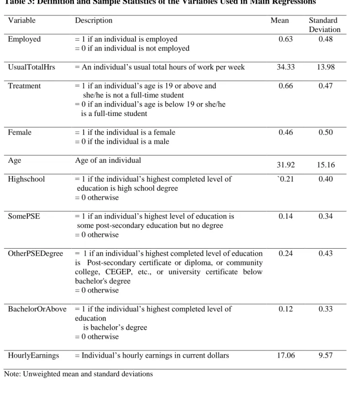
(14) The amount of the benefit depends on family structure. Except for Alberta and Québec, all other provinces have two schemes of benefit- one for single persons and the other for families (i.e., single parents with eligible children and couples with or without children). Alberta’s two schemes are for single persons and couples, while Québec has four schemes- single without eligible children, couples without eligible children, single parents with eligible children and couples with eligible children. The federal government allows provinces and territories to modify the design of the WITB to better harmonize it with provincial and territorial programs, given that such changes improve work incentives for low-income individuals and families, are cost neutral to the federal government, provide for a minimum benefit level for all WITB recipients, and preserve harmonization of the WITB with existing federal programs (Federal Budget, 2007). By January 2015, Alberta, British Columbia, Quebec, and Nunavut had modified the WITB. These modifications include changes in the minimum earnings threshold, phase-in and phase-out rate, maximum benefit amount etc. However, none of these provincial variations is important for my estimation procedure since all these modified programs maintain same qualitative implication for labour supply, and I estimate average effect of the WITB for the whole Canada. To qualify for the WITB benefit, an individual or a family must have working income over a minimum level. For each dollar of working income over the minimum threshold, they receive a certain percentage of it as the WITB (phase-in), until they reach the maximum benefit. Once they reach the maximum benefit, their benefit remains constant (plateau) until their working income reaches another threshold after which the benefit starts decreasing (phase-out) at a certain percentage of each additional dollar. Once the benefit starts decreasing, it continues to decrease until it reaches another threshold where they no longer become eligible for any benefit. These thresholds, phase-in rate and phase-out rates depends on family structure and varies across provinces. Initially the program was smaller. For the federal structure of the WITB, the maximum benefit in 2007 was $500 for single individuals without dependents and $1,000 for couples and single parents. This maximum amount was increased in 2009 to $925 for single individuals without dependents and $1,680 for couples and single parents. The maximum benefit continues to increase each year at the rate of inflation. Figure 1 shows the federal structure of the WITB for a single person in 2013. In the federal structure of the WITB, a single individual requires to exceed the minimum working income threshold of $3,000. Once the working income exceeds this minimum. 5.

(15) threshold, the individual receives 25 cents for each additional dollar (phase-in). Once working income reaches $6,956, the benefit level reaches the maximum benefit of $989. The benefit level then remains unchanged until working income reaches $11,231 (plateau). For each additional dollar of working income exceeding the $11,231 plateau, the benefit reduces by 15 cents (phase-out). Finally, the benefit reduces to zero when working income reaches $17,825.. 4. THEORETICAL BACKGROUND In a standard textbook model of the labour-leisure trade-off, the introduction of the WITB expands the budget set of eligible individuals. The idea can be best illustrated with the help of a diagram. In Figure 2, the vertical axis represents an individual’s total endowment of time. If all time is spent on leisure, the individual has no income. If the individual sacrifices leisure hours to work, he or she receives income. A part of the income goes to government as tax, and the individual can consume the after tax income. The possible combinations of labour and after tax income that the individual can choose defines the budget line EF. For an eligible individual, the WITB expands his or her budget line. Once an individual works enough hours to reach the minimum threshold to receive the WITB, he or she starts receiving an income supplement for each dollar earned beyond the minimum threshold (phase-in). The individual continues getting this supplement until their income reaches the lower limit of the income range where one is eligible to receive the maximum amount of WITB, which happens when the individual works ED hours. For each additional dollar they earn after that, they no longer receive any further credit but continues getting the maximum amount (the plateau). In the diagram, this situation corresponds to the RQ part of the budget line. After that, each additional dollar earnings reduces their credit, and the credit completely phases out when the individual’s earning reaches a certain amount (phase-out). In the diagram, the corresponding labour hour is EA. So, introduction of WITB makes paid work more attractive since all individuals are becoming at least as well off as before. As a result, all individuals who preferred working before the introduction of the WITB will still prefer working, while the additional income from the WITB might become pivotal in some individuals’ decision of participating into paid work. So, from theory, the WITB has no reason to decrease employment, and is likely to increase it. 6.

(16) On the other hand, how the WITB affects an individual already in the labour force depends on the region where the individual remains before the initiation of the program. First, an individual in AB (the phase-in) region faces both income and substitution effects. The credit works as a subsidy to wage, so the opportunity cost of a leisure hour becomes higher for the individual. As a result, the individual gets incentive to reduce leisure hours and increase labour hours. This is the substitution effect. On the other hand, since leisure is generally considered a normal good, the additional income from the WITB incentivize the individual to get more leisure time and work less. This is the income effect. So, for phase-in region, the income and substitution effects work against each other and the effect of hours for individuals in this region is ambiguous from the theory. Second, if the individual is originally in BC (the plateau) region, the WITB only causes an income effect that motivates the individual to increase leisure hours and reduce labour hours. Third, if the individual is originally in CD (the phase-out) region, the additional money from the credit causes a negative income effect on hours of work. Also, the phase-out nature of the credit acts as a disincentive for work. So, the WITB motivates the individuals originally in the phase-out region to reduce hours of work. Thus, on average whether the WITB increases hours of work is ambiguous from the theory. It depends on whether the income effect and the substitution effect dominates in the phase-in region, and the relative number of individuals in these regions.. 5. DATA 5.1. Data Source I use confidential microdata from the Labour Force Survey (LFS). The LFS is a national monthly household survey that represents 98 percent of the Canadian population. Each monthly round of the LFS consists of nearly sixty thousand individuals. The LFS follows a stratified sampling process and the data are collected primarily from phone interviews during the week following the LFS reference week, which is normally the week containing the 15th day of the month. Each selected household is interviewed six months in a row. If a member moves out from a selected household in between this six month periods, he or she is no longer followed. On the other hand, if someone moves in, he or she is surveyed for the remaining months. Since younger people moves much more frequently than older people, exploiting any panel nature of the LFS might face a significant attrition bias. In this study, I combine all monthly surveys from January 2004 to December 2013. 7.

(17) Since individual identifier is not readily available from the LFS microdata, I do not perform any individual-level clustering, rather I consider each observation as independent. Such assumption pose my estimation to the risk of getting underestimated error terms. Therefore, I also run same regressions while clustering the errors on household level or provincial level. In most of the cases, resulting standard errors increases, but not enough to have a large impact on the statistical significance of estimated coefficients. I elaborate these robustness checks in section 7.3.. 5.2. Sample Selection Since I aim to explore the effect of the WITB on employment and hours of work, first I naturally restrict the sample to the working-age population, aged between 15 and 64, inclusive. I also restrict my sample to unattached individuals (i.e., neither married nor in a common-law relationship) to avoid complications arisen from couples’ joint labour supply decision. I further restrict my sample to the individuals who do not have a child below 19 years of age because otherwise a good portion of the treatment group population qualifies for three other of three other programs that might affect their labour supply as well and thus pose a threat to my identification. These programs are the National Child Benefit (NCB), National Child Benefit Supplement (NCBS), and Child Tax Credit. In 2005 and 2006, the NCB amounts was increased by 14 percent and 13 percent respectively. Also in 2009, the NCB threshold was increased by 11.4 percent. Between 2005 and 2006, the maximum income threshold for the NCBS, which is a component of the Canada Child Tax Benefit (CCTB), was lowered twice by 5 percent. In 2007 the Child Tax Credit, which is a non-refundable tax credit of $2000 for the parents and guardians of children under 18 years of age, was introduced. Although families do not require to participate in the workforce to become eligible for these programs, Milligan and Stabile (2007) pointed that in many provinces socials assistance is clawed back at a sharp rate, and as result, these programs influence the decision to enter into paid work. Thus, I will not be able to disentangle the effect of the WITB from these programs, unless I drop the people with young children from my sample.. 5.3. Sample Characteristics In my main sample, 62.68 percent people are employed, who on average work around 34 hours per week. 66.41 percent people of the sample, who represent the treatment group, are 19 years or older,. 8.

(18) and not a full-time student. 46.34 percent people in the sample are female while 54.64 percent are male. Average age of the people in the sample is around 32 years. For 20.67 percent people, high school degree are their highest level of education. 13.52 percent people have some post-secondary education but no diploma, while 23.91 percent have a post-secondary certificate or diploma, or community college degree, CEGEP, etc., or university certificate below bachelor's degree. 12.46 percent people have bachelors or higher degrees. From the LFS, hourly earnings is available for employed employees only, and the average hourly earnings is 17.05 dollar, measured in current terms. In Table-1 I summarize the sample means and standard deviations of the variables used in my main regressions.. 6. EMPIRICAL FRAMEWORK 6.1. The Estimand: What I Estimate The causal effects of the WITB on employment and hours of work could have been best estimated if, in addition to observing the states of employment and hours of work after the program was introduced, we also observe the states of employment and hours of work in otherwise same environment if the WITB were not introduced Fundamental Problem of Causal Inference (Holland, 1986). However, the quasi-experimental nature of the program and the LFS microdata allows me to estimate a particular type of causal effect of the WITB. In this paper, I identify the average treatment effect on the treated (ATET) of the WITB on the intensive and extensive margins of the labour supply. In less technical words, I estimate the average impact of the WITB on eligible single individuals’ employment and hours of work.. 6.2. Difference-in-differences Since its introduction by Ashenfelter and Card (1985), the difference-in-differences is a popular method for empirical evaluation in a quasi-experimental setting. This method can perform causal estimation under an assumption weaker than the OLS conditional exogeneity assumption. The method requires a treatment group and a control group, and at least two periods of panel or repeatedcross sectional data- one before and one after the program was introduced. The difference-indifferences method identifies average treatment effect on the treated (ATET) under the assumption 9.

(19) that, the counterfactual trend of the treatment group would have been parallel to the realized trend of the control group. In other words, this assumption implies that the outcomes may differ in level between the treatment and the control groups, but no other factors than the program to evaluate should affect the outcomes differently in the treatment and control groups. Suppose that Y is the outcome in question. Subscripts T and C indicate treatment and control groups respectively. Subscript 1 indicates observation after the program is introduced while subscript 0 indicates observation before the program was introduced. So, 𝑌̅T, 0 and 𝑌̅T, 1 are the average outcomes of the treatment group before and after the program was introduced respectively, and (𝑌̅T, 1. - 𝑌̅T, 0) is the difference between these average outcomes. This difference indicates how the. average outcome evolved for the case of treatment group. In a similar fashion, 𝑌̅C, 0 and 𝑌̅C, 1 are the average outcomes of the control group before and after the program was introduced respectively, and (𝑌̅C, 1 - 𝑌̅C, 0) is the difference between these average outcomes. This difference indicates how the average outcome evolved for the case of control group. [(𝑌̅T, 1 - ̅𝑌T, 0 ) − (𝑌̅C, 1 - 𝑌̅C, 0)] is the difference in these two differences. This term shows how bigger or smaller is the overtime change in the outcome of the treatment group than the overtime change in the outcome of the control group. Under the assumption that other than the program, all other factors affect both groups equally, this difference-in-differences is the average treatment effect on the treated (ATET). 𝐴TET = (𝑌̅T, 1 - ̅𝑌T, 0 ) − (𝑌̅C, 1 - 𝑌̅C, 0) = (𝑌̅T, 1 - ̅𝑌C, 1 ) − (𝑌̅T, 0 - 𝑌̅C, 0) This ATET is equivalent to the parameter β3 of the following linear regression: Y = β0 + β1 Treatment + β2 Post + β3 Treatment * Post + u. (1). Y is the outcome, β0 is an intercept and u accounts for all other relevant variables not included as regressor. The coefficient on Treatment dummy, β1, represents the average initial difference in the untreated outcome between the treatment and control groups. The coefficient on Post dummy, β2, represents the average difference in the untreated outcome between the observations before and after the program was introduced. The coefficient on the interaction between the Treatment dummy and Post dummy, Treatment * Post, is β3, which is the difference-in-differences parameter and represents how the average difference in outcome between the treatment and control groups changed after the program was introduced. Under the assumption that no other factor other than the 10.

(20) program can affect the outcome differently in treatment and control groups, this β3 identifies the ATET. One can also incorporate control variables in equation (1). In that case, the ATET can is identified under even a further weaker assumption that conditional upon the controls, no other factor other than the program can affect the outcome differently in treatment and control groups. This is the assumption behind my main regressions since the LFS data allows me to control for some relevant variables.. 6.3. Specifying Main Regressions 6.3.1. Variable Definitions Employed and UsualTotalHrs are my outcome variables. Employed is a binary variable that takes 1 if an individual is employed, where UsualTotalHrs is an individual’s usual total hours of work per week. For difference-in-differences design, I generate three variables: Treatment, Post, and Treatment*Post. The variable Treatment is an indicator that shows if an individual in my sample is eligible for the WITB. This indicator takes value 1 if an individual’s age is 19 or above and she/he is not a full-time student, and takes 0 if an individual’s age is below 19 or she/he is a fulltime student. Post is another binary variable, which indicates if an individual is observed after the WITB is introduced. It takes value 1 if an individual is observed in 2007 or later, and takes 0 otherwise. The variable Treatment*Post is an interaction term between Treatment and Post. This interaction term takes 1 when both Treatment and Post takes 1, and takes 0 when any of the Treatment and Post takes 0. Among the control variables, Female indicator takes 1 if the respondent is a female. Age represents an individual’s age in years where Age-squared is the square of age. For capturing the effect of education, I consider non-completion of high school degree is base category, and generate four education dummies: Highschool, SomePSE, OtherPSEDegree, and BachelorOrAbove. The Highschool dummy takes 1 if an individual’s highest level of education is a high school degree, and takes zero otherwise. The SomePSE dummy takes 1 if an individual’s highest level of education is some post-secondary education but not any post-secondary degree, and takes 0 otherwise. The OtherPSEDegree indicator takes 1 if an individual’s highest completed level of education is postsecondary certificate or diploma, or community college, CEGEP, etc., or university certificate 11.

(21) below bachelor's degree, and takes 0 otherwise. The dummy BachelorOrAbove takes 1 if the individual’s highest completed level of education is bachelor’s degree or more, and takes 0 otherwise. To estimate the effect of the WITB on hours of work, I control for HourlyEarnings, hourly earnings of an individual in dollar. However, the LFS has this data for all employed employees including those who receives compensation on a yearly basis. So, while this HourlyEarnings represents wage for the individual and might be exogenous, for others this HourlyEarnings is derived from dividing total income by total hours and thus endogenous. I also use year dummies and province dummies to control for aggregate time effects and province specific factors respectively.. 6.3.2. Effect on Employment My first set of regressions estimate the effect of the WITB on eligible single individuals’ employment. I first estimate linear difference-in-differences models of the following form using OLS: Employed =  + ϒ1 Treatment + ϒ2 Post + ϒ3 Treatment * Post + βZ + u. (2). Then, since Employed, is a binary variable, I also estimate probit models designed with the difference-in-differences techniques: Employed = ( + ϒ1 Treatment + ϒ2 Post + ϒ3 Treatment * Post + βZ + u). (3). Here Employed, Treatment, Post and Treatment * Post are as defined in Section 6.3.1. While for the linear model in equation (2), the coefficient on Treatment * Post, ϒ3, directly represents the ATET, for the probit model showed in equation (3), I instead calculate the Average Marginal Effect of Treatment * Post. In both models, Z is a vector of control variables that includes a female dummy, age, age-squared, education dummies, year dummies, and province dummies. The female dummy is naturally excluded when dealing with the split sample of only males or only females.. 6.3.3. Effect on Hours of Work My second set of regressions estimate the effect of the WITB on eligible single individuals’ hours of work. I estimate linear difference-in-differences models of the following form using OLS: UsualTotalHrs =  + ϒ1 Treatment + ϒ2 Post + ϒ3 Treatment * Post + βZ + u. 12. (4).

(22) Here UsualTotalHrs, Treatment, Post and Treatment * Post are as defined in Section 6.3.1., and the coefficient on Treatment * Post, ϒ3, directly represents the ATET. First, I consider the case of a combined sample of males and females, and use two specifications. In both specifications, the vector of control variables, Z, includes female dummy, age, age-squared, education dummies, year dummies, and province dummies. However, these two specifications differ in terms of controlling for hourly earnings, and also they deal with different samples. The LFS has hours of work data for all employed people covered by the survey. However, since for the self-employed people, it is hard to differentiate earnings and profit, hourly earnings data is available for the employed employees only. Thus, one of these two specifications does not control for hourly earnings and deals with the sample of all employed individuals, and the other specification controls for hourly earnings and deals with the sample of employed employees only. Then I split the sample between males and females, and use the same two specifications except for naturally excluding the female dummy.. 6.4. Potential Endogeneity from Self-selection of the Treatment In the above mentioned regressions, I assume that the decision to enroll as a full-time student and labour supply decisions are independently made. Such assumption is similar to the frequently made assumption in the evaluation of the EITC or the WFTC that whether a women is childless single or a single mother is not influenced by their decision to determine whether to enter into paid work or how many hours to work, but the other way around. If the decision to enroll as a full-time student and labour supply decisions are jointly made, my empirical framework suffers from an endogeneity problem.. 6.5. Incorporating IV Strategy with the Difference-in-Differences Design I present an instrumental variable strategy to encounter this potential endogeneity problem. Unfortunately, I can apply this instrumental variable strategy to only a subset of my samplesindividuals aged 18 and 19 years old.. 6.5.1. The Instruments and the 2SLS Estimation If the decision to enroll as a full-time student is jointly made with the labour supply decisions, the variables Treatment and Treatment * Post become endogenous. To solve this potential endogeneity problem, I consider a sub-sample consist of people of age 18 and 19 years only. I use Age19, which. 13.

(23) is an indicator for 19 years old, as an instrument for Treatment, and Age19*Post as an indicator for Treatment * Post. Using these instruments, I estimate the causal effect of the WITB using two-stage least squares. In the first first-stage regression, I run endogenous regressor Treatment on instruments and exogenous regressors. In the second first-stage regression, I run endogenous regressor Treatment*Post on instruments and exogenous regressors. From these first stage regressions, I find fitted values of Treatment and Treatment*Post, and using the fitted values I run the endogeneity corrected difference-in-differences regressions. This instrumental variable strategy requires precisely coding the individuals based on whether they are 18 or 19 years old. From the LFS, I do cannot access an individual’s exact birth date. Rather what is available is an individual’s age in years in the week before the LFS survey takes place. Since an individuals’ age on 31st December is taken into account while determining his or her WITB eligibility, for the sake of assigning the treatment accurately, I use only December rounds of the LFS for this instrumental variable strategy, while as a robustness check I use the November rounds only.. 6.5.2. Excludability and Relevance Conditions of the Instruments From a labour market perspective, whether an individual of 18 years and an individual of 19 years are no different, once I control for their sex and whether they are a high school dropout. So, I can exclude age from the regressions that estimate the effect of WITB on employment and hours of work. Thus, the exclusion condition of an instrumental variable is likely to hold for my instruments. On the other hand, these instruments are likely to have a strong positive correlation with the potentially endogenous regressors, which I later confirm from the data. So, the relevance condition of an instrumental variable is also satisfied.. 6. 6. Use of Weights The LFS is not a random sample. Some regions are over-sampled in the LFS, while some regions are under-sampled. As a result, an unweighted regression is unlikely to estimate population parameters. In the Labour Force Survey (LFS), the sampling error and part of the error due to household nonresponse are dealt with by attaching an estimation weight called final weight (Statistics Canada, 2008). In all regressions, I use this final weight as the probability weight.. 14.

(24) 7. RESULTS I report my main findings in Section 7.1. In Section 7.2, I report results from instrumental variable strategy applied to a sub-sample of young singles of 18 and 19 years of age. In Section 7.3. I describe robustness checks.. 7.1. Main Findings 7.1.1. Effect of the WITB on Employment I report the results from difference-in-differences regressions in Table 4. First, I take men and women together and run Linear and Probit models using difference-in-differences design. Then, I split the sample between men and women and re-run the regressions. Men and Women Together: The first column of results in Table 4 is from the linear model. The estimated coefficient on Treatment is 0.259, which implies that even without the treatment an individual in the treatment group is 25.9 percentage points more likely to be employed than a similar individual in control group. So, there is a considerable gap between the employment rate of the treatment and control groups, and a simple cross-sectional study with similarly defined treatment would dramatically overstate the true effect of the WITB. The coefficient on the interaction term between Treatment and Post, which is my coefficient on interest, is 0.010. As I describe in Section 6, this coefficient indicates the average treatment effect on the treated (ATET). This coefficient implies the WITB increases the likelihood of an eligible individual to be in paid work by 1.0 percentage points. This result is statistically significant at 1 percent level. Among the control variables, the coefficient on Female is 0.034, which implies that women are 3.4 percentage points more likely to be employed. This might be less surprising than as it seems, since the sample deals with single people with no young children. The coefficients of age and age-squared are positive and negative respectively, which shows diminishing effect of age on the probability of being employed. All education dummies have positive coefficients, implying people within these categories are more likely to be employed than people who did not complete high school degree, the base category. 15.

(25) In the second column of results, I report average marginal effects from the probit model. The estimated coefficient on Treatment is 0.245, which implies that individuals who are in treatment group are 24.5 percentage points more likely to be employed. This effect is close to its linear counterpart and statistically significant at 1 percent level. The estimated coefficient on the interaction term between Treatment and Post is 0.006, which implies the WITB on average increases the likelihood of employment for eligible individuals by 0.6 percentage point, which is a little smaller in magnitude than its linear counterpart and statistically significant at 1 percent level. In case of control variables, the signs, magnitude and statistical significance closely resemble the linear model. Men Only: Next I split the sample by sex. In the third and fourth columns of Table 4, I report difference-indifferences results from the linear and probit models for men. In the linear model, the coefficient on Treatment is 0.298 which implies that even without the treatment an individual in the treatment group is on average 29.8 percentage points more likely to be employed than a similar individual in control group. This effect is around 4 percentage points greater than what I get for the sample of both sexes. The coefficient on the interaction term between Treatment and Post is 0.004, which implies the WITB on average increases the probability of employment among the individuals in the treatment group by 0.4 percentage points, which is statistically significant at 5 percent level and smaller than its counterpart from the combined sample. The effects of the control variables and their statistical significance resemble the case of combined sample. In the probit model, the coefficient on Treatment is 0.272, which implies a man being in treatment group is on average 27.2 percentage point more likely to be employed than a similar individual in the control group. This effect is statistically significant at 1 percent level and greater than the case of combined sample. In contrast to the combined sample case, the estimated coefficient on the interaction term between Treatment and Post is negative. However, this coefficient is not statistically significant and the confidence interval lies very close to zero. Women Only: I report results from the women only sample in the fifth and sixth columns of results in Table 4. In the fifth column, I report results from the linear model. The coefficient on Treatment is 0.21 which implies even without the treatment a woman being in the treatment group is 21 percentage points more likely to be employed. The estimated coefficient on the interaction term between Treatment. 16.

(26) and Post is statistically significant at 1 percent level. This coefficient implies that the WITB on average increases the probability of being employed among treated women by around 2 percentage points. In column six, I report average marginal effects from the probit model for women. The coefficient on Treatment implies a woman in treatment group is on average 20.9 percentage points more likely to be employed than a similar woman in control group. The coefficient on the interaction term between Treatment and Post is 0.016, which implies the WITB on average increase the likelihood of being employed among women in treated group by 1.6 percentage points. The estimated effect of the control variables are statistically significant at 1 percent level. To summarize the effect of the WITB on employment, for the combined sample the WITB increases the probability of participating into paid work by 0.6 percentage point according to the probit model and 1 percentage points according to the linear model. These effects are statistically significant at 1 percent level. When the sample is split between men and women, the effect among treated men is almost zero, and statistically significant at 10 percent and insignificant according to the linear and probit models respectively. However, in case of women, according to both the linear and probit models, the effect is statistically significant at 1 percent level, and greater in size than that of men. From the t-statistics of coefficient heterogeneity, I find that difference in the effect of the WITB is statistically significant. So, the effect on employment that I estimate from the combined sample is mostly driven by women.. 7.1.2. Effect of the WITB on Hours of Work I run linear difference-in-difference regressions to estimate the effect of the WITB on total usual work hours per week. The LFS contains usual total hours per week for all employed people, but hourly earnings for employed employees only. So, I am able to control for hourly earnings for the latter group only. I, thus, first run regressions on all employed people where I do not control for hourly earnings. Then I employ same regressions but control for hourly earnings on the sample of employed employees. I report my findings in Table 5. (Case 1) When Hourly Earnings Is Not Controlled and the Sample Consists of Employed People: The first three columns of Table 5 results from a sample of employed employees, where I control for hourly earnings. Men and Women Together:. 17.

(27) The coefficient on Treatment is 12.97, which indicates even without treatment an individual in treatment group on average works 12.97 hours more than a similar individual in the control group. This effect is statistically significant at 1 percent level. The estimated coefficient on the interaction term between Treatment and Post is 0.38, which implies the WITB increases usual work hours per week by 0.38 hours. The effect is statistically significant at 1 percent level. Among the control variables, the coefficient on the female dummy indicates women on average work 3.46 hours less than similar men. The positive coefficient on age and negative coefficient on age-squared implies diminishing effect of age on hours of work. The positive coefficients on the education dummies indicate individuals having high school or higher degrees work more hours than those who did not complete a high school degree. Men Only: When running the difference-in-differences regression on the sample of employed males, the coefficient on Treatment implies that even without treatment men in the treatment group on average work 13.74 hours more than similar men in the control group. This effect is statistically significant at 1 percent level. The coefficient on the interaction term between Treatment and Post is 0.13, which implies the WITB increases usual work hours per week by 0.13 hours among treated men. The qualitative implications of the coefficient on control variables and their statistical significance resemble the case of combined sample. Women Only: In case of employed females, the coefficient on Treatment implies even without treatment the treated females on average work 12.10 hours more than similar non-treated females. The coefficient on the interaction term between Treatment and Post is 0.63, which implies the WITB increases usual work hours per week by 0.63 hours among treated females. Qualitative implications of the coefficient on control variables and their statistical significance resembles the case of combined sample. (Case 2) When Hourly earnings is Controlled and The Sample Consists of Employed Employees: Table 5 also includes differences-in-differences estimations of the effect of the WITB on the usual total hours per week using a sample of employed employees, where I control for hourly earnings. When Men and Women are Taken Together:. 18.

(28) The coefficient on Treatment is 12.72, which indicates even without treatment an individual in the treatment group on average works 12.72 hours more than a similar individual in the control group. This effect is statistically significant at 1 percent level. The coefficient on the interaction term between Treatment and Post is 0.45, which implies the WITB increases usual work hours per week by 0.45 hours. The effect is statistically significant at 1 percent level. Among the control variables, the coefficient on female dummy indicates women on average works 3.46 hours less than similar men. The positive coefficient on age and negative coefficient on age-squared implies diminishing effect of age on hours of work. The positive coefficients on the education dummies indicate individuals having high school or higher degrees work more hours than those who did not complete high school degree. The coefficient on hourly earnings is positive, as expected. All these coefficients of controls are statistically significant at 1 percent level. Men Only: When run difference-in-differences regression on the sample of employed males, the coefficient on Treatment implies that even without the treatment the treated males on average work 13.36 hours more than similar non-treated males. This effect is statistically significant at 1 percent level and around one hour more than its combined sample counterpart. The estimated coefficient on the interaction term between Treatment and Post is 0.45, which implies the WITB increases usual work hours per week by 0.45 hours among treated males. Qualitative implications of the coefficient on control variables and their statistical significance resembles the case of combined sample. Women Only: In case of employed females, the coefficient on Treatment implies even without the treatment, the treated females on average works 11.94 hours more than similar non-treated females. This effect is smaller than the case of men. The coefficient on the interaction term between Treatment and Post is 0.67, which implies the WITB increases usual work hours per week by 0.67 hours among treated females. This effect is around a half hour greater than the effect on men. The qualitative implications of the coefficient on control variables and their statistical significance resemble the case of combined sample. To summarize the effect on hours of work, I found the WITB on average increased usual hours of work per week by around 23-27 minutes for the combined sample of men and women. For men, this average increase is around 7-15 mines, while for women this average increase is 38-40 minutes. From a test of coefficient heterogeneity I find the higher effect among women is statistically. 19.

(29) significant at 5 percent level. So, the effect on hours of work that I estimate from the combined sample is mostly driven by women.. 7.2. Results When IV Strategy Is Incorporated As discussed in Section 6.4, individuals can self-select the treatment by altering their decision to be a full-time student, which might be jointly determined with their decision to participate in paid work, or how many hours to work. To handle this potential endogeneity problem, I use the instrumental variable strategy described in Section 6.5, which is applicable to only a sub-sample consist of individuals of age 18 and 19 years. I use Age19 and Age19*post as instruments for Treatment and Treatment*Post respectively, and employ 2SLS estimation as described in Section 6.5. In all first stage regressions, I find my instruments strong (correlation coefficient with the endogenous regressors is around 0.5 in most of the cases), and statistically significant.. 7.2.1. Effect of the WITB on Employment In Table 6, I report difference-in-difference regressions of the effect of the WITB on employment on a sample of childless singles aged 18 and 19 years. In the first column I report the OLS coefficients, while in the second column I report the second stage regression coefficients. From the IV regressions. In both of these cases, I control for an indicator for sex and whether an individual is a dropout form high school. According to the OLS estimation, the coefficient on Treatment is 0.254, which, which implies even without treatment an individual in treatment group is 25.4 percentage points more likely to be employed than a similar individual in control group. The coefficient on the interaction term between Treatment and Post is -0.026, which implies that the WITB decreased the probability of getting employed among the treated individuals by 2.6 percentage points. This negative effect is contradictory to the prediction from the theory described in section 4. However, this effect is not statistically significant. In the second column, I report the endogeneity corrected results from the second stage regression of the 2SLS estimation. The coefficient on Treatment is now 0.147, which implies an individual in the treatment group is 0.147 percentage points more likely to be employed than a similar individual in control group. The coefficient on the interaction term between Treatment and Post is -0.028 which implies the WITB on average decreases the probability of participating into paid work by 20.

(30) 2.8 percentage points, which is a little greater effect than the OLS case. However, this negative effect is contradictory to the prediction from the theory, and not statistically significant. In the third column, I also report the OLS reduced form results. In contrary to the first column, here I use Age19 instead of Treatment, and Age19*Post instead of Treatment*Post. The coefficient on Age19 is 0.062, which implies, that even without the treatment, an individual who is 19 years old is 6.2 percentage points more likely to be employed than a similar individual who is 18 years old. The coefficient on the interaction term between Age19 and Post is -0.015, which implies that, after the WITB was introduced, the 19 years old individuals are 1.5 percentage points less likely to become employed than similar individuals who are 18 years old. This effect is smaller than the ATET estimated in the first column. However, this effect is not statistically significant either.. 7.2.2. Effect of the WITB on Hours of Work Same as the main regressions, while looking at the effect of the WITB on hours of work, I use two samples- employed individuals and employed employees, where I can control for hourly earnings for the latter only. (Case 1) When Hourly Earnings is Not Controlled and the Sample Consists of Employed People: In Table 7, I first report OLS results from the sample of employed individuals of age 18-19. The coefficient on Treatment implies that even without the treatment individuals in treatment group on average work 11.77 hours more than similar individuals in the control group. The coefficient on the interaction term between Treatment and Post is -0.39, which implies the WITB reduced usual hours of work per week by 0.39 hours. However, this effect is not statistically significant. In the second column, I report the endogeneity-corrected results from the second stage regression of the 2SLS estimation. The coefficient on Treatment implies that even without the treatment individuals in treatment group works on average 4.92 hours more than similar individuals in the control group. The coefficient on the interaction term between Treatment and Post is -1.06, which implies the WITB reduced usual hours of work per week by 1.06 hours. This effect is smaller than its OLS counterpart, and as in the OLS case, is not statistically significant. In the third column, I also report the OLS reduced form results. The coefficient on Age19 implies that, even without the treatment, individuals who are 19 years old on average work 2.65 hours more than similar individuals who are 18 years old. The coefficient on the interaction term between Treatment and Post is -0.71, which implies that after the introduction of the WITB, 19 years old individuals work 0.71 hours less per week compared to similar individuals who are 18 years old. 21.

(31) This effect is larger than the ATET measured in the first column. However, this effect is not statistically significant either. (Case 2) When Hourly Earnings is Controlled and the Sample Consists of Employed Employees: In the fourth column of Table 7, I report the difference-in-differences regression results using OLS on a sample of employed employees. The coefficient on Treatment is 11.27, which implies that individuals in the treatment group work on average 11.27 hours more than similar individuals in the control group. The coefficient on the interaction term between Treatment and Post is -0.63, which implies the WITB reduced usual hours of work per week by 0.63 hours. This effect is not statistically significant. In the fifth column, I report endogeneity-corrected difference-in-differences regression results using 2SLS. The coefficient on Treatment implies that even without treatment the individuals in treatment group work on average 4.04 hours more than similar individuals in the control group. The coefficient on the interaction term between Treatment and Post is -1.28, which implies the WITB reduced usual hours of work per week 1.28 hours. This effect is greater than its OLS counterpart, and as in the OLS case, is not statistically significant. In the sixth column, I also report the OLS reduced form results. The coefficient on Age19 implies that, even without the treatment, individuals who are 19 years old on average work 2.14 hours more than similar individuals who are 18 years old. The coefficient on the interaction term between Treatment and Post is -0.78, which implies that after the introduction of the WITB, 19 years old individuals work 0.78 hours less per week compared to similar individuals who are 18 years old. This effect is larger than the ATET measured in the first column. However, this effect is not statistically significant either. To summarize the IV findings, among the group of single, childless individuals of age 18 and 19, the endogeneity corrected difference-in-differences coefficients representing the average treatment effect of the WITB on the treated individuals’ employment and usual hours of work per week are negative, small and statistically insignificant. Although this IV design is a solution for the potential endogeneity problem arisen from the self-selection of the treatment, my estimated coefficients of interests are not statistically significant. Also, my IV results cannot be compared with the results obtained from my main sample, since they are limited to the people of age 18 and 19 only.. 22.

(32) 7.3. Robustness Check I perform four robustness checks for the main specifications described in Section 7.1. First, I conduct a placebo test. Using only observations from 2004 to 2006, which are the years before the introduction of the treatment, I estimate regressions in Section 7.1., where I intentionally consider 2004 and 2005 as the pre-treatment years and 2006 as the post-treatment year. Since there was actually no treatment in 2006, if my difference-in-difference design is correct, I should not get any treatment effect for 2006. This anticipation is confirmed by the data since the size of the estimated effects become close to zero and statistically insignificant. Second, in contrast to using heteroskedasticity robust standard error, I cluster the errors at the provincial level. The estimated standard errors increases and most of the estimated effects at the extensive margin no longer remain statistically significant at the 5 percent level but most of the estimated effects the estimated effects at the intensive margin remains statistically significant. Third, I cluster the errors by household. At the extensive margin, according to the linear model, similar to the case without clustering, the estimated effect of the WITB is statistically significant at 1 percent level if both sexes are taken together. However, if the effect is estimated separately in men and women, the effect no longer remains statistically significant at 10 percent, whereas it is statistically significant at 10 percent in the case without clustering. According to the probit models, if both sexes are taken together, statistical significance increases to 10 percent level, whereas it was 1 percent in the case without clustering. However, when the effect is estimated separately in men and women, clustering on household does not cause any important change. At the intensive margin, clustering on household level does not cause any important change if both sexes are taken together, or if only women are considered. However, in the sample of employed men, contrary to its without clustering counterpart, the estimated effect no longer remains statistically significant at 10 percent level. Also, in the sample of male employed employees, statistical significance increases to 10 percent level, whereas it was 1 percent in the case without clustering. I report these results in Table 8 and Table 9. Fourth, I relax my specifications by interacting provincial dummies with year dummies. Such flexible specification, which allows the time differential effect of the provincial variations, does not meaningfully change the size of the estimated effects, and the almost all the effects still remain statistically significant at 5 percent level.. 23.

(33) 8. CONCLUDING REMARKS This paper is the first study to my knowledge that uses actual behavioural data to investigate how the WITB affected the extensive and intensive margins of labour supply. To disentangle the effect of the WITB from the effects of other programs, I restrict my analysis to a sample of working-age, unattached individuals with no children below 19 years living with them. The quasi-experimental structure of the program allows me to construct a treatment and a control group, since eligibility for the program requires individuals be over 19 years of age and not a full-time student. I employed difference-in-differences techniques and used the Labour Force Survey (LFS) confidential microdata. At the extensive margin, using difference-in-differences technique with linear and probit models, I find the WITB increased the probability of being employed by up to around two percentage points. At the intensive margin, using linear difference-in-differences models, I find the WITB increased usual hours of work per week by up to around forty minutes. In both margins, the labour supply response is greater for women, and this difference in response is statistically significant. An in-work tax credit like the WITB is likely to affect labour supply of the following groups most: single mothers, women with young children, and second earners. However, I restricted my analysis to working-age, unattached individuals with no children below 19 years living with them. Given this fraction of population is likely to have a high participation rate in the workforce even before the program introduced, the estimated average increase in their employment probability by up to two percentage points is not negligible. Also, since there are opposing income and substitution effects in case of the effect of this program on the hours of work, and many jobs hardly allow over time, in my opinion, the estimated average increase in usual hours of work per week by up to around forty minutes is sizable. Thus, from these estimates, I think the WITB has been successful in stimulating labor supply, at least within a portion of the population. Now I conclude this paper discussing some points related to the strength and weakness of my estimation, and shedding light on avenues for future research. First, unlike most of the EITC and the WFTC studies, my treatment and control groups are not constructed depending on having children. The positive side of having such treatment and control groups is that my estimation is not contaminated from the effects of many other programs that are contingent on having children. The negative side is that, since most of the individuals in my treatment group are mature individuals while most of the individuals in my control group are young people, my treatment and control. 24.

(34) groups are more likely to be affected differently by factors other than the WITB and thus the underlying counterfactual parallel trend assumption of difference-in-differences might be violated. Future work on the labour market changes focusing on these treatment and control groups could help readers to better decide how much they should rely on the parallel trend assumption. Second, I did not control for macroeconomic variables directly, but rather used time and province dummies to control for aggregate effects. Although such flexible specification helps to avoid assuming adhoc fictional relationship, since the period of my analysis includes recession and recovery periods, explicitly modeling macroeconomic factors in the evaluation of the WITB might be an avenue for future research. Third, the eligibility condition for the WITB depends on whether an individual is a full-time student. If this decision that might be jointly determined with labour supply decisions, my estimation suffers from endogeneity problem. Although I can argue for the exogeneity of the treatment along the lines of the exogenous fertility decision assumption commonly made in the EITC evaluations, I outline an instrumental variable strategy to encounter this potential endogeneity problem. I present an arguably sound instrumental variable strategy but my instrumental variable strategy is applicable to a small subsample consists of only young people, who might not be well aware of tax benefits. Thus, finding instruments that are applicable for a wider population could be another worthwhile initiative for future work.. 25.

No results found