A computationally fast variable importance test for random forests for high-dimensional data

(1)

Silke Janitza, Ender Celik, Anne-Laure Boulesteix

A computationally fast variable importance test for random

forests for high-dimensional data

Technical Report Number 185, 2015 Department of Statistics

University of Munich

(2)

A computationally fast variable importance test

for random forests for high-dimensional data

Silke Janitza

∗

Ender Celik

Anne-Laure Boulesteix

October 22, 2015

Department of Medical Informatics, Biometry and Epidemiology, University of Munich, Marchion-inistr. 15, D-81377 Munich, Germany.

Abstract

Random forests are a commonly used tool for classification with high-dimensional data as well as for ranking candidate predictors based on the so-called variable importance measures. There are different importance measures for ranking predictor variables, the two most com-mon measures are the Gini importance and the permutation importance. The latter has been found to be more reliable than the Gini importance. It is computed from the change in predic-tion accuracy when removing any associapredic-tion between the response and a predictor variable, with large changes indicating that the predictor variable is important. A drawback of those variable importance measures is that there is no natural cutoff that can be used to discriminate between important and non-important variables. Several approaches, for example approaches based on hypothesis testing, have been developed for addressing this problem. The existing testing approaches are permutation-based and require the repeated computation of forests. While for low-dimensional settings those permutation-based approaches might be computa-tionally tractable, for high-dimensional settings typically including thousands of candidate predictors, computing time is enormous. A new computationally fast heuristic procedure of a variable importance test is proposed, that is appropriate for high-dimensional data where many variables do not carry any information. The testing approach is based on a modified version of the permutation variable importance measure, which is inspired by cross-validation procedures. The novel testing approach is tested and compared to the permutation-based test-ing approach of Altmann and colleagues ustest-ing studies on complex high-dimensional binary classification settings. The new approach controlled the type I error and had at least com-parable power at a substantially smaller computation time in our studies. The new variable importance test is implemented in theRpackage vita.

Keywords: Gene selection, Feature selection, Random forests, Variable importance, Variable

selection, Variable importance test.

(3)

1

Introduction

Since its introduction in 2001 random forests have evolved to a popular classification and regression tool which is applied in many different domains. A random forest is a collection of decision trees that are built from a subset of the original data (Breiman; 2001). In contrast to many parametric methods, random forests can deal with nonlinear effects and it is often claimed that interactions are adequately taken into account (see, Boulesteix et al.; 2015, for a recent discussion on this issue). Random forests are fully non-parametric and thus offer a great flexibility. Moreover, they

can even be applied in the statistically challenging setting in which the number of variables,p, is

higher than the number of observations, n. This makes random forests especially attractive for

complex high-dimensional molecular data applications. Fast implementations of random forests are already available (e.g., Wright and Ziegler; 2015; Schwarz et al.; 2010).

A further advantage of random forests is that they also offer so-called variable importance measures which can be used to rank variables according to their predictive abilities. Often, identifying relevant genes is of high interest to gain valuable insights into the functionality and mechanisms that lead to a specific disorder. Moreover, the identification of relevant genes aids in the diagnosis of certain disorders. The random forests method and its implemented importance measures have often been used for the identification of such biomarkers (e.g., Reif et al.; 2009; Wang-Sattler et al.; 2012; Yatsunenko et al.; 2012).

There are two commonly used variable importance measures, the Gini importance and the permutation importance. Several articles have shown that the Gini importance has undesirable properties (Strobl et al.; 2007; Nicodemus and Malley; 2009; Nicodemus; 2011; Boulesteix, Bender, Bermejo and Strobl; 2012). For example variables that offer many cutpoints systematically obtain higher Gini importance scores (Strobl et al.; 2007). Thus the permutation variable importance should be preferred. The permutation variable importance measure – also referred to as the mean decrease in accuracy – reflects the average decrease in accuracy when destroying the association between a variable and the response by permuting the values of the variable. It is clear that predictor variables whose importance score is negative or zero are likely to have no predictive ability. However, for the predictor variables with positive importance score it is difficult to say which importance scores are large enough so that it is unlikely that these have occurred by chance. The variable importance depends on several different factors, including factors related to the data, such as correlations between the data, the signal-to-noise ratio or the total number of variables, and including forest specific factors, such as the choice of the number of randomly drawn candidate predictor variables for each split. Therefore there is no universally applicable threshold that can be used to determine what really high importance scores are.

Often, in practical applications, a certain percentage of the highest ranked variables are se-lected; Reif et al. (2009) for example filtered out the 10% of variables with the highest importance scores and used them for further considerations. However, one should be careful when selecting a pre-specified number of highest ranked variables and considering these as relevant because one would always identify some variables as relevant even in the absence of any associations between the variables and the disorder.

An ad-hoc approach consists in using the absolute value of the smallest observed importance score as a threshold for determining which variables are likely to be relevant, because one can be sure that the smallest observed importance score must have been occurred due purely to chance (Strobl et al.; 2009). However, this approach has several disadvantages, two of them being that

(4)

the threshold depends on one single observed importance score and that it becomes more extreme the more variables there are. It is thus clear that more elaborated approaches are needed.

Testing procedures are a sensible strategy for deciding which variables are likely to be relevant (Saeys et al.; 2012). In a statistical test we aim to draw conclusions about the value of a population parameter through the use of the observed sample. In the context of variable importance it is not clear what this population parameter refers to and if it even exists. Thus the testing approaches that were proposed for random forest’s variable importance measures, should rather be regarded as heuristic methods that enable the selection of variables, instead of real statistical tests in the strict mathematical sense. However, for simplicity and to be consistent with the literature, we will refer to such approaches as statistical tests in this paper, although it should be kept in mind that in the strict mathematical sense these are not statistical tests.

A statistical test based on the supposed normality of a scaled version of the permutation variable importance was proposed by Breiman (2008). However, the procedure of Breiman (2008) has been shown to have alarming statistical properties, and should not be used (Strobl and Zeileis; 2008). During the last years, more and more approaches have been developed that test which variables are related to the outcome (see Hapfelmeier and Ulm; 2013, and references therein). Since the true null distribution of variable importance depends on various factors, it becomes difficult – if not impossible – to theoretically derive the null distribution. This is the reason for the frequent use of permutation strategies in the existing testing approaches (Tang et al.; 2009; Altmann et al.; 2010; Hapfelmeier and Ulm; 2013). However, such procedures are computationally demanding. Very recently Hapfelmeier and Ulm (2013) published a comprehensive comparison study of different permutation-based testing approaches. They conclude that their novel approach has higher statistical power than many of the existing approaches and controls the type I error. Their approach works as follows: For each variable that is tested for its association with the response, a large number of forests (Hapfelmeier and Ulm (2013) used 400 in their studies) has to be computed. Each forest is constructed based on a different permuted version of the variable

and the importance score of the permuted version is computed. The p-value for the variable is

then computed as the fraction of variable importance scores (obtained for the permuted versions), that are greater than the variable importance of the original (i.e., unpermuted) version of the

variable. The computation ofp-values for all variables thus requires computing as many forests

as predictor variables multiplied by the number of permutation runs. This approach has been developed and investigated for the classical low-dimensional setting which typically includes not more than a dozen covariates. It is obvious that with high-dimensional data such permutation-based approaches become very computationally demanding, and might even become practically unfeasible.

In this paper we present a heuristic variable importance test for high-dimensional data that is computationally very fast and particularly suitable for high-dimensional genomic data. This test is based on a slightly modified version of the permutation variable importance measure. Note that the permutation variable importance measure is the method of first choice for an importance measure

since it is almost unbiased (see, e.g., Boulesteix, Janitza, Kruppa and K¨onig; 2012). In contrast

to the existing approaches, our testing procedure is not based on permutations. The idea of this novel testing procedure is to use the information of observed non-positive variable importance scores to reconstruct the null distribution of variable importance. This null distribution is then

used to compute p-values. We show results of several studies that explore if the new testing

(5)

The power of our novel testing approach is also compared to the power of the permutation-based testing approach of Altmann et al. (2010). The approach of Altmann et al. (2010) has often been used since its introduction in 2010 (e.g., Polak et al.; 2015; Prosperi et al.; 2014). It is very computationally demanding, especially for high-dimensional data settings. But compared to the approach of Hapfelmeier and Ulm (2013) it is computationally feasible for high-dimensional data settings. Therefore we only consider the testing approach of Altmann et al. (2010) as a competing method.

This paper is structured as follows: In Section 2 we briefly review the idea of random forests, their integrated permutation variable importance measure and the heuristic testing approach of Altmann et al. (2010). Then we present a heuristic testing idea which is applied to the classical permutation variable importance measure (“naive approach”). As will be shown the testing idea is based on presumptions which are not met by the classical permutation variable importance measure. We therefore present a modified version of the classical permutation variable importance which fulfills the criteria. Subsequently we introduce our novel testing procedure which is based on this modified version of the permutation importance. Moreover, in Section 2 we describe the designs considered in the simulation studies, which are conducted for testing our novel testing approach and for the comparison to the naive approach and the approach of Altmann et al. (2010). Section 3 shows the results of our studies and Section 4 gives a brief summary and discussion of our results.

2

Methods

2.1

Random Forests

Random forests is an ensemble method that combines several classification trees. It can be used for classification and regression tasks as well as for more special analyses such as for survival analysis (Ishwaran et al.; 2008; Hothorn et al.; 2006) and ordinal regression (Hothorn et al.; 2006; Janitza et al.; 2015). In this paper we focus on the use of random forests for classification tasks. Each tree in random forests is built from a bootstrap sample or from a subsample of the original data.

The observations that are not used for the construction of a specific tree are termedout-of-bag

(OOB) observations. At each split in a tree a subset ofmtry predictor variables is drawn from all

candidate predictors and considered for the split. Among those variables, the one that provides the “best” split is selected. There are different variants of random forests, which basically differ in their splitting criteria. The most popular variant is that of Breiman (2001), which implements splits based on node impurity measures, such as the Gini index for classification trees. Another popular variant proposed by Hothorn et al. (2006) is based on hypothesis testing. The variant of Hothorn et al. (2006) has been shown to yield an unbiased split selection, while the classical variant of random forests (Breiman; 2001) tends to favor variables that offer many split points.

For our studies we used the classical random forest variant of Breiman (2001) implemented in

theRpackage randomForest (Liaw and Wiener; 2002). Though this variant implements a biased

split selection, we chose it for implementing our studies because of its computational speed. With respect to computing time, the random forest implementation of Breiman (2001) by far outper-forms the (unbiased) random forest implementation of Hothorn et al. (2006). Since we consider settings with a very large number of covariates and repeatedly fit random forests, the unbiased random forest variant of Hothorn et al. (2006) is not applicable due to its high computational

(6)

effort. However, we tried to avoid affecting our results by the biased split selection by choosing only settings with continuous predictor variables so that we did not expect that a split selection bias would occur in our studies. Moreover, we used subsampling (i.e., sampling from the original data without replacement) instead of bootstrapping in order to avoid possible biases induced by the bootstrap (Strobl et al.; 2007).

2.2

Classical permutation variable importance

Random forests offer variable importance measures which can be used to rank variables according to their predictive abilities. The idea underlying the permutation variable importance measure is to compare the prediction errors made by trees before and after permuting the values of a specific predictor variable. By permuting the values of a predictor variable, we make sure that the variable is not related to the response after the permutation. If the variable was associated with the response before permutation, and if this relation is destroyed by permutation, the discrepancy between the trees’ prediction errors before and after the permutation of the predictor variable will be large. In contrast, if the predictor variable is just noise, a permutation of the variable’s values will not affect the trees’ prediction errors. Usually the prediction error of trees is measured by the misclassification rate for categorical responses. The classical permutation variable impor-tance measure is then computed from the difference in misclassification rates before and after the permutation: V Ij= 1 ntree ntree_X t=1 1 |OOBt| X i∈OOBt {I(yi6= ˆyit∗)−I(yi 6= ˆyit)}, (1)

withI(.) denoting the indicator function,OOBt denoting the set of indices for observations that

are out-of-bag for treet∈ {1, . . . , ntree}, and ˆyitand ˆyit∗ denoting the predictions by thet-th tree

before and after permuting the values of the variableXj, respectively.

In this paper a variable is termed as relevant if the trees’ prediction errors significantly increase after the random permutation, or equivalently, if the variable significantly improves the prediction accuracy. It is important to note that this definition of relevant predictor variables also includes variables that do not have their “own” effect on the response, but are associated with the response due to their correlation with truly influential predictor variables.

From the definition of the variable importance measure, it is clear that negative values or values of zero indicate that the variable does not improve the trees’ predictive abilities, because on average the error rates are similar or even larger when using the original, i.e., unpermuted version of the variable. Thus we infer that the variable is likely to not be relevant. A positive value for the variable importance, in contrast, reflects that the variable at least slightly improves the trees’ predictive abilities since the error rates are smaller on average when using the original version of the variable for deriving tree predictions. However, one cannot infer that a positive value for the variable importance indicates a relevant variable since we do not know if the change in prediction errors is solely due to chance. Testing procedures are required to assess if the change in error rates is significantly larger than zero. If it is the case we can infer that the variable is likely relevant.

(7)

2.3

Permutation-based testing approach of Altmann et al. (2010)

The testing approach of Altmann et al. (2010) has originally been proposed as heuristic for correct-ing biased importance measures, such as the Gini importance measure. However, it is applicable to all kinds of importance measures of random forests. Besides its ability to correct biased

im-portance measures, it outputsp-values which are computed from importance scores. This feature

enables the user to select relevant variables based on thep-values.

In the first step of the method of Altmann et al. (2010), the variable importance scores are obtained for all variables. Any arbitrary importance measure may be used for computing the importance scores – it may even be biased. In the second step, importance scores for settings in which the variable is not associated with the response are computed. Altmann et al. (2010) generate these settings by randomly permuting the response variable to break any associations between the response variable and all predictor variables. The data generated in this way is then used to construct a new random forest and to compute the importance scores for the predictor variables. The importance scores can be regarded as realizations drawn from the unknown null distribution. The procedure, which involves the steps of randomly permuting the response vector,

constructing a random forest and computing the importance scores, is repeatedS times. For each

variable there areSimportance scores that can be regarded as realizations from the unknown null

distribution. Finally, in the last step of the method of Altmann et al. (2010), theS importance

scores are used to compute thep-value for the variable. One possibility for deriving thep-value

consists in computing the fraction of S importance scores that are greater than the original

importance score. This approach is referred to as thenon-parametricapproach in this paper since

we do not make any assumptions on the distribution of importance scores of unrelated predictor variables. Alternatively, one can assume a parametric distribution such as the Gaussian, Log-normal or Gamma-distribution for the importance scores of unrelated predictor variables. The parameters for the respective distribution are replaced by their maximum likelihood estimates,

which are computed based on theSimportance scores of the considered variable. Having defined a

specific distribution for the variable’s null importance, thep-value is computed as the probability

of observing an importance score that is higher than the original importance score, given this

distribution. We refer to this approach asparametric approach.

2.4

Naive testing approach

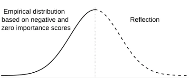
From its definition, the classical permutation variable importance is expected to randomly vary around the value zero if variables are not associated with the response. In this paper we investigate a new heuristic approach which consists in approximating the null distribution based on the ob-served non-positive importance scores. More precisely, we reconstruct the variable importance null distribution by mirroring the empirical distribution of the observed negative and zero importance

scores on they-axis. This results in a distribution which is symmetric around zero (see Figure

1). Let M1 = {V Ij|V Ij < 0;j = 1, . . . , p} denote the observed negative variable importance

scores, andM2={V Ij|V Ij= 0;j = 1, . . . , p}is the set of importance scores which are zero, with

p denoting the number of candidate predictors. We define the hypothetical importance scores

M3 ={−V Ij|V Ij <0;j = 1, . . . , p} =−M1, which arise from multiplying the negative

impor-tance scores by₋1. The null distribution ˆF0is computed as the empirical cumulative distribution

(8)

Variable importance 0

Empirical distribution based on negative and zero importance scores

Reflection

Figure 1: Reconstruction of the null distribution based on variables that are likely non-relevant (i.e., with negative or zero importance scores). The negative part of the null distribution (solid line) is approximated based on the observed negative and zero importance scores. The positive

part (dashed line) is obtained from reflection about they-axis.

Based on ˆF0 ap-value for variableXj is derived as

pj= 1−Fˆ0(V Ij).

It is clear that this testing approach is not suitable for all types of data. The data must contain a relatively large number of variables without any effect so that the approximation of the null distribution is precise enough. A high number of variables without any effect is typically present with genetic data, such as microarray or SNP data, so that our testing approach is primarily of practical relevance to high-dimensional genomic data settings.

2.5

Novel permutation variable importance

The novel variable importance measure is not based on the out-of-bag observations but uses a similar strategy, which is inspired by the cross-validation procedure. In a nutshell the idea is as

follows: We first split the data intok sets of equal size. We then constructk forests, where the

l-th forest is constructed based on observations that are not part of the l-th set. For each forest

we then use observations for variable importance computation that were not used for constructing the forest.

Let Sl contain the indices of observations from the l-th set, and|Sl| denotes the cardinality

of Sl. For categorical response the fold-specific variable importance for predictor variable Xj is

defined by V I_jCV(l)= 1 ntree ntree_X t=1 1 |Sl| X i∈Sl {I(yi6= ˆyit∗)−I(yi6= ˆyit)}, (2)

withntree denoting the number of trees in a forest, I(.) denoting the indicator function and ˆyit

and ˆy∗

it denoting the predictions by the t-th tree before and after permuting the values of Xj,

respectively. Note that the predictions ˆyit and ˆy∗it, t= 1, . . . , ntree, are obtained from the forest,

which is constructed based on observations_{1,2, . . . , n_}\Sl, and thus does not use the observations

i∈Sl in tree construction.

Thecross-validated variable importance for predictor variableXj is then defined by

V IjCV = 1 k k X l=1 V IjCV(l). (3)

(9)

The most simple version of cross-validation results for k= 2, so that each of the two sets is once used for creating the forest and once for deriving importance scores. In general, this method is also known as 2-fold validation or the hold-out method. To differentiate it from

cross-validation withk≥3, from now on we will refer to it as the hold-out method. The corresponding

hold-out variable importancefor predictor variableXj is given by

V IjHO= 1 2 2 X l=1 V I_jCV(l), (4)

and directly results from settingkto 2 in Eq. (3). Thus it is a special case of the cross-validated

importance measure defined in Eq. (3).

2.6

New testing approach

The new testing approach solely differs from the naive testing approach in the fact that it uses the hold-out variable importance (Eq. (4)) instead of the classical out-of-bag-based importance (Eq. (1)). The hold-out importance measure is preferred over the classical importance measure in the new testing approach because it has desirable properties as will be shown in this paper.

Based on the hold-out variable importance, thep-values are derived in exactly the same

man-ner as for the naive approach. The basic steps of our novel testing approach are sketched in the following.

A novel variable importance test for high-dimensional data

Step 1 The data is randomly partitioned into two sets of equal size. Each set is used to create a

random forest. The two forests are used to compute the hold-out variable importanceV IHO

j

(see Eq. (4)) for variablesXj, j= 1, . . . , p.

Step 2 The null distribution for the hold-out variable importance is approximated based on the

observed non-positive importance scores. For this purpose we define the sets

M1={V IjHO|V IjHO<0;j= 1, . . . , p}(i.e., all negative importance scores),

M2={V IjHO|V IjHO= 0;j= 1, . . . , p}(i.e., all importance scores of zero) and

M3 ={−V IjHO|V IjHO <0;j = 1, . . . , p} =−M1 (i.e., all negative importance scores

multiplied by−1),

and consider the empirical cumulative distribution function ˆF0 ofM =M1∪M2∪M3.

Step 3 Thep-value corresponding to the variable importance of predictor variable Xj is computed

as

pj= 1−Fˆ0(V IjHO).

Note that in this paper we use the hold-out version of the classical permutation variable importance which uses the difference in error rates before and after randomly permuting the values of the considered variable. Our proposed testing procedure is very general in the sense that hold-out versions of different permutation-based variable importance measures might be used, such as the conditional permutation importance of Strobl et al. (2008), the AUC-based importance of

(10)

Janitza et al. (2013), or the importance measures for ordinal responses considered in Janitza et al. (2015).

It is important to note that if one wants to use a different measure, say, the conditional importance of Strobl et al. (2008), the hold-out version of this measure should be computed, that is, the variable importance should be computed using the splitting procedure described in 2.5.

The new testing approach is implemented in theRpackage vita, which is based on theRpackage

randomForest (Liaw and Wiener; 2002). Currently, only the hold-out version of the classical

variable importance measure is implemented. TheRpackage vita also contains an implementation

of the testing approach of Altmann et al. (2010).

2.7

Simulation studies

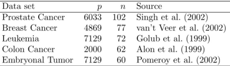
Since our new testing approach is suitable for high-dimensional genomic data, we only consider settings with large numbers of predictor variables and high signal-to-noise ratios. There is common consensus in the literature that it is very difficult – if not impossible – to simulate realistic complex data structures which capture all the patterns and sources of variability that are generated by a real biological system. Therefore we based our studies on five high-dimensional genomic data sets from real world applications (see Table 1 for an overview). These data sets were often used by various authors for binary classification purposes (e.g., D´ıaz-Uriarte and De Andres; 2006; Dettling and

B¨uhlmann; 2003; Tan and Gilbert; 2003). A brief description of the data sets is given in Appendix

A. Note that no pre-selection of data sets based on the results was done, instead we report the results of all data sets that we analyzed, as has been recommended by Boulesteix (2015).

Data set p n Source

Prostate Cancer 6033 102 Singh et al. (2002)

Breast Cancer 4869 77 van’t Veer et al. (2002)

Leukemia 7129 72 Golub et al. (1999)

Colon Cancer 2000 62 Alon et al. (1999)

Embryonal Tumor 7129 60 Pomeroy et al. (2002)

Table 1: Overview over high-dimensional genomic data sets used for our investigations. p: number

of predictor variables;n: number of observations in the considered data set.

To study the properties of our test, we need to know which of the variables are truly relevant and which are not. In other words, we have to know the truth, which we can never know from real world data. Therefore in our studies we used the design matrix of the real world data sets, but the response vector was generated anew according to a specified relation. Three different studies were performed. Table 2 gives an overview of the three studies.

Predictor variables Correlations between

with effect predictor variables

Study I no yes

Study II yes yes

Study III yes no

Table 2: Overview of performed studies which differ in the inclusion of predictor variables with effect and in the presence of correlations between predictor variables.

In the first study (Study I) none of the predictor variables of a data set has an effect and there are correlations between predictor variables. In the second and third studies (Study II, III)

(11)

some of the predictor variables have an effect on the response. While Study II includes correlated variables, in Study III all predictor variables are independent of each other.

We tested our novel testing procedure and the naive testing procedure using Studies I, II and III. To obtain stable results we performed the computations for 500 repetitions of each study. Due to computational reasons, we performed only 200 repetitions of each study for the approach of Altmann et al. (2010). We used the permutation importance defined in Eq. (1) for computing

p-values according to the approach of Altmann et al. (2010). This enables a fair comparison of

our novel approach, which is based on the permutation variable importance measure, and the

approach of Altmann et al. (2010). We always computed p-values for both approaches

(non-parametric and (non-parametric). Altmann et al. (2010) point out that a Kolmogorov-Smirnov test might be used to choose the most appropriate distribution for the parametric approach. In our studies we adhere to Algorithm 1 (outlined in the Supplement to Altmann et al.; 2010), which uses a Gaussian distribution with mean and variance estimated by the arithmetic mean and sample

variance, respectively. The parameter S should be chosen so that it is large enough. For the

parametric approach the recommendation of Altmann et al. (2010) is a valueS between 50 and

100. No recommendations were given for the non-parametric method. We always used a large

valueS= 500 in the studies to exclude the possibility that the performance of Altmann’s approach

may be related to a suboptimal choice of parameters. In the following we describe each study in more detail.

2.7.1 Study I

The first study reflects scenarios where all predictor variables are pure noise. We used the original design matrix and the original response vector of the real data applications. To destroy associations between the response vector and the design matrix we permuted the elements of the response vector. In this modified data, associations between predictor variables and the response are only due to chance. Note that the design matrix was not modified and correlations between predictor variables were preserved.

2.7.2 Study II

In our second study we simulated a scenario in which 100 variables have an effect on the response and the other variables have no effect. We again used the original design matrix reflecting realistic correlation patterns, but generated a new response vector. This allows for a complex data scenario, but at the same time we have the information which of the variables are relevant.

The binary response Y for an observation with covariate vector x> _{= (}_x

1, x2, . . . , xp) was

generated from a logistic regression model with success probability

P(Y = 1_|x) = exp(x1β1+x2β2+. . .+xpβp)

1 + exp(x1β1+x2β2+. . .+xpβp)

,

withpdenoting the total number of predictor variables in the considered data set. The coefficients

β1, β2, . . . , βp were chosen as follows: First we randomly drewj1, j2, . . . , j100 without replacement

from the set _{1,2, . . . , p_} to define which of the variables have an effect on the response and

should therefore be selected by a variable importance testing procedure. The corresponding

co-efficientsβj1, βj2, . . . , βj100 were subsequently drawn from the set {−3,−2,−1,−0.5, 0.5,1,2,3},

(12)

zero.

Although standardization is not necessary for the application of random forests in general, we standardized the design matrix in order to make effects comparable across variables of different scales.

2.7.3 Study III

This study includes only uncorrelated predictor variables. We used the design matrix of the real data sets and permuted the values within each variable independently to create uncorrelated variables. As with Study II, 100 variables were supposed to have an effect on the response. The approach for deciding which variables have an effect and for generating the response is exactly the same as described for Study II.

2.7.4 Parameter settings

We performed analyses under different parameter settings to see if the choice of parameters affects the results. All studies (Studies I, II, III) were performed

• for two different values for the parametermtry: mtry =√pandmtry =p₅, withpdenoting

the number of predictor variables.

• for two different numbers of predictor variables. We used either a very large number of

candidate predictors, namely that from the original design matrices (see Table 1), or a

subset of p = 100 predictor variables randomly drawn from the original design matrices.

In the studies with large predictor numbers 100 variables had an effect, and in the studies

with a subset ofp= 100 predictor variables only 20 variables had an effect (only relevant to

Study II and III).

• for two different sets that both determine the effects of relevant predictor variables (only

relevant to Study II and III). One set was chosen as _{−3,₋2,₋1,₋0.5, 0.5,1,2,3_}. A

second effect set with smaller effects was also investigated: {−1,−0.8,−0.6, −0.4,−0.2,

0.2,0.4,0.6,0.8,1_}. Since results were very similar for the two different sets, only those for

the effect set{−3,−2,−1,−0.5, 0.5,1,2,3} are shown.

The number of trees in the random forest was always set to 5000. We used subsamples of size

d0.632n_eto construct trees, withndenoting the number of total observations (Strobl et al.; 2007).

All other parameters not mentioned here were set to the default values so that trees were grown to

maximal depth. The codes implemented in our studies can be obtained from the websitehttp://

www.ibe.med.uni-muenchen.de/organisation/mitarbeiter/070_drittmittel/janitza/index. html.

2.7.5 Evaluation criteria

One important aspect that was investigated in the studies is the statistical power of the testing approaches. The statistical power is generally defined as the probability of rejecting the null hypothesis, given that the null hypothesis is false. In this paper we define the null hypothesis that the trees’ prediction accuracy does not worsen when permuting the values of a predictor variable. If the null hypothesis is rejected (i.e., prediction accuracy worsens), there is evidence that the variable is relevant. The statistical power of the testing approaches was explored by

(13)

computing the fraction of variables with p-value below α = 0.05 of those that have an effect. Note that in Studies II and III there are predictor variables with different effect strengths; the

absolute effect strengths are 0.5,1,2,3, or 0.2,0.4,0.6,0.8,1 in the alternative setting. For power

considerations we computed the proportion of variables withp-value belowα= 0.05 within each

subset of variables with the same absolute effect.

The second important aspect concerns the validity of the testing approaches. The type I error of a test is defined as the probability of rejecting the null hypothesis, given that the null hypothesis

is true. A test is valid if its type I error does not exceed the significance levelα. In our studies we

investigated if the testing procedures control the type I error by computing the fraction of variables

withp-value belowα= 0.05 among those variables that are not relevant. For this purpose we had

to know which variables are not relevant. In Study I none of the variables has an effect and thus none is relevant. In Study III exactly those variables whose regression coefficient is zero are not relevant. In Study II, however, due to the correlation between the variables, it is difficult to assess which variables are not relevant: Predictor variables that do not have an “own” effect (i.e., those with coefficient of zero) but are correlated with variables that have an effect, might significantly improve the trees’ predictive abilities. Therefore in Study II, the regression coefficients cannot be used to judge which variables are not relevant, because variables with coefficients of zero can also be relevant. Thus only Study I and III can be used for investigating the type I error.

In addition to type I error and power investigations, we inspected two further related issues. The first issue concerns the assumption of the presented testing procedure that under the null hypothesis the variable importance distribution is symmetric around zero. We empirically assessed if this is the case for the variable importance measures introduced in Sections 2.2 and 2.5 by plotting the distribution of variable importance scores observed in Study I, where none of the variables is relevant. If we observe an asymmetric distribution or a distribution which is shifted

along thex-axis, we expect the testing procedure to have a systematically too high or too low

type I error.

The second issue concerns the discrimination between relevant and non-relevant variables by their importance scores. A testing procedure will have low statistical power if it is based on a variable importance measure that does not discriminate well between relevant and non-relevant variables. Thus we inspected the discriminative ability to see if the novel hold-out variable impor-tance may be used in a testing procedure. We considered the classical permutation imporimpor-tance as “gold standard” and compared its discriminative ability to that of the hold-out importance. For these investigations we used Study III because, in contrast to Study II, we know which variables are relevant and which are not. The area under the curve was used as a measure for

discrimi-native ability. Let the predictor variable indices B =_{1, . . . , p_} be partitioned into the disjoint

setsB=B0∪B1, whereB0represents the non-relevant variables andB1 represents the relevant

variables. The area under the curve is defined by

AU C= 1 |B0| |B1| X j∈B0 X k∈B1 I(V Ij < V Ik) + 0.5I(V Ij=V Ik) (5)

where_|Bl|denotes the cardinality of Bl with l ∈ {0,1}, and I(·) denotes the indicator function

(see, e.g., Pepe; 2004). Note that the area under the curve is often used for evaluating the ability of a method (which may be for example a diagnostic test or a prediction model) to correctly discrim-inate between observations with binary outcomes (often diseased versus healthy). In our studies,

(14)

as the units to be predicted (as relevant or non-relevant variables) rather than the observations

i= 1, . . . , n. The area under the curve here corresponds to an estimate of the probability that a randomly drawn relevant variable has a higher importance score than a randomly drawn non-relevant variable. An AUC value of 1 means that each of these non-relevant variables receives a higher importance score than any non-relevant variable, thus indicating perfect discrimination by the im-portance measure. An AUC value of 0.5 means that a randomly drawn relevant variable receives a higher importance score than a randomly drawn non-relevant variable in only half of the cases, indicating no discriminative ability by the importance measure.

3

Results

3.1

Properties of the classical and novel permutation importance

3.1.1 Null distribution

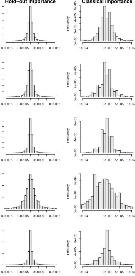
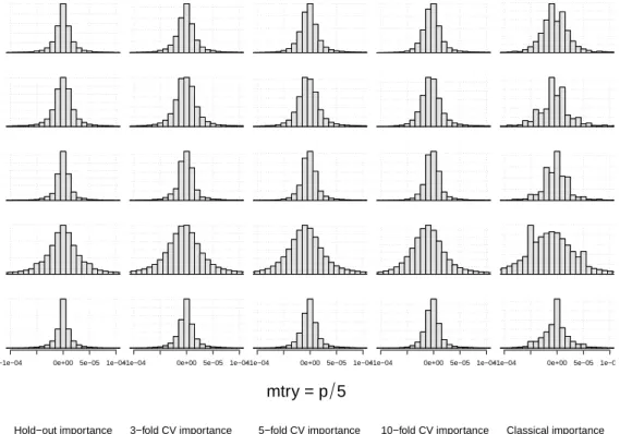
Figure 2 shows the null variable importance distributions for the novel hold-out variable impor-tance (left panel) and the classical variable imporimpor-tance (right panel) for the settings with large

predictor space andmtryset to√p. Results are very similar formtry=p₅ and are shown in Figure

B.1 in the appendix.

The null distribution of the hold-out variable importance seems to be symmetric around zero, and thus seems to satisfy the presumption of a symmetric null distribution. In contrast to that, the null distribution of the classical variable importance is not totally symmetric. In the studies

withp= 100 this asymmetry is much more apparent (Figure B.9): All distributions are clearly

positively skewed showing that a large fraction of variables have small negative importance scores, while smaller fractions of variables have large positive importance scores. The null distribution of

the cross-validated variable importance looks very similar fork≥3 (see Figures B.1, B.9). In

con-trast, the null distribution of the fold-specific variable importance is nearly symmetric around zero (results not shown). This seems to be contradictory since the cross-validated variable importance is the average of fold-specific variable importances. Further inspection of the simulation results

reveals that this effect is possibly due to the overlap of forests. Fork_≥3 the same observations

are used for creating the forests of several folds. For example, if we had three sets,S1, S2, S3, the

first forest is constructed usingS2 and S3, the second forest is constructed using S1 andS3, and

the third forest is based onS1 andS2. Each pair of forests have some part of the observations in

common. For example, the first and the second forests are both based on observations from set

S3. The variables have similar predictive abilities for the sets S2∪S3 (on which the first forest

is trained) andS1∪S3 (on which the second forest is trained). If high values for a variable Xj

speak in favor of class 1 in the subsetS2∪S3, then in the subsetS1∪S3high values forXj will

also speak in favor of class 1 – even if there is, in reality, no association betweenXj and the class

membership. Even in settings without any associations, the two forests then often select the same

predictor variables for a split. Thus fork_≥3 one of the same few variables will always obtain high

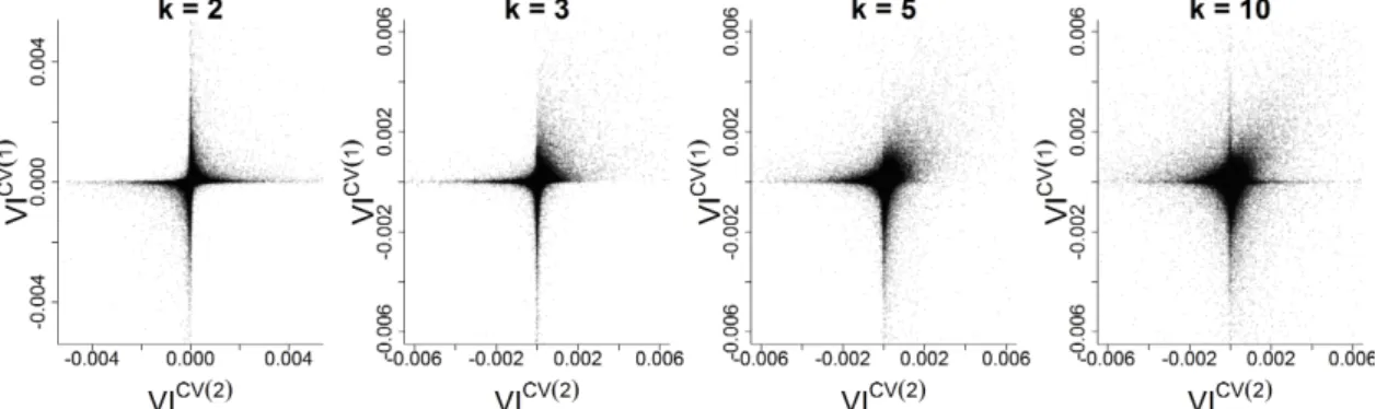
specific importance scores as can also be seen from empirical studies. In Figure 3 the fold-specific variable importance scores for the first two folds (for the Colon Cancer data) are plotted

against each other for different values of k. The fold-specific variable importance computed for

500 repetitions of Study I (no relevant variables) withmtry set to p₅ are shown. Results formtry

=√pare shown in Figure B.2. Similar results are obtained for the other data sets and when using

(15)

Hold−out importance

unlist(sapply(studyI_cv2_smallmtry_prostate, function(z) z$cv_varim))

Frequency −0.00015 −0.00005 0.00005 0.00015 0e+00 4e+05 8e+05 Prostate Cancer

Classical importance

unlist(studyI_classical_smallmtry_prostate) Frequency

−1e−04 0e+00 5e−05 1e−04

0e+00

2e+05

4e+05

6e+05

unlist(sapply(studyI_cv2_smallmtry_breast, function(z) z$cv_varim))

Frequency −0.00015 −0.00005 0.00005 0.00015 0e+00 2e+05 4e+05 6e+05 Breast Cancer unlist(studyI_classical_smallmtry_breast) Frequency

−1e−04 0e+00 5e−05 1e−04

0e+00

2e+05

4e+05

unlist(sapply(studyI_cv2_smallmtry_leukemia, function(z) z$cv_varim))

Frequency −0.00015 −0.00005 0.00005 0.00015 0 400000 1000000 Leuk emia unlist(studyI_classical_smallmtry_leukemia) Frequency

−1e−04 0e+00 5e−05 1e−04

0e+00

4e+05

8e+05

unlist(sapply(studyI_cv2_smallmtry_colon, function(z) z$cv_varim))

Frequency −0.00015 −0.00005 0.00005 0.00015 0 50000 150000 Colon Cancer unlist(studyI_classical_smallmtry_colon) Frequency

−1e−04 0e+00 5e−05 1e−04

0e+00 4e+04 8e+04 Frequency −0.00015 −0.00005 0.00005 0.00015 0 500000 1500000 Embr y onal T umor Frequency

−1e−04 0e+00 5e−05 1e−04

0e+00

4e+05

8e+05

Figure 2: Variable importance null distribution when using the classical permutation variable importance measure and the novel hold-out permutation variable importance measure and setting

mtryto √p(default value). Distributions are shown for all variables and 500 repetitions (Study

(16)

clearly observe the phenomenon just described: There are some variables which have large positive fold-specific variable importance scores for both folds resulting in a large cross-validated variable importance score. In contrast, there are not as many variables with negative fold-specific variable importances for both folds. From that it is clear that the cross-validated variable importance has a skewed null distribution.

Figure 3: Fold-specific variable importance for the first fold plotted against fold-specific variable

importance for the second fold for Study I (mtry = p₅) of the Colon Cancer data with k = 2,

k= 3,k= 5 andk= 10.

We expect that similar mechanisms occur with the classical permutation variable importance, which is based on the out-of-bag observations, as the classical permutation variable importance

is similar to the cross-validated variable importance in whichk is set to the sample sizen. But

more research is needed to fully understand the behavior of the classical permutation variable importance.

The hold-out variable importance, in contrast, is not affected in the same manner. Here the

data is partitioned into the setsS1andS2. Each set – and correspondingly each observation within

the set – is used for the construction of one forest. The first forest usesS2 and the second forest

usesS1, resulting in two forests which are completely independent of each other. The selection of

variables for a split in the second forest is thus independent of which variables have been selected

in the first forest. Therefore the mechanisms described fork _≥3 do not apply for k = 2. This

is also supported by the empirical results in Figures 3 and B.2 (first plot) where we observe an equal amount of variables with negative fold-specific variable importance scores for both folds as variables with positive fold-specific importance scores for both folds. Although, we note a substantially higher number of variables with both negative or positive fold-specific importance scores than variables with one negative and one positive fold-specific importance score. This might be explained by the fact that the variable importance for the first forest is computed using

observations from setS1, that have been used for the construction of the second forest, and vice

versa. A positive correlation might therefore be expected between the fold-specific importance scores. However, this has no effect on the symmetry of the null distribution of the hold-out variable importance.

To conclude, we have empirically shown that the hold-out variable importance has a symmetric null distribution, while the classical importance and the cross-validated variable importance do not have a symmetric distribution. From our studies we would expect that our novel testing approach controls the type I error exactly, while the naive testing approach does not.

(17)

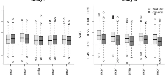
● ● ● ● ● ● ● ● ● ● ● ● ● ● ● ● ● ● ● ● ● ● ● ● ● ● ● ● ● ● ● ● ● ● ● 0.45 0.50 0.55 0.60 0.65 Study II A UC

Prostate Cancer Breast Cancer

Leuk emia Colon Cancer Embr y onal T umor ● ● ● ● ● ● ● ● ● ● ● ● ● ● ● ● ● ● ● ● ● ● ● ● ● ● ● ● ● ● ● ● ● ● ● ● ● ● ● ● ● ● ● ● ● 0.45 0.50 0.55 0.60 0.65 Study III A UC

Leuk emia Colon Cancer Embr y onal T umor hold−out classical

Figure 4: Discriminative ability of the novel hold-out permutation variable importance measure and the classical permutation variable importance measure. Discriminative ability is measured by

the area under the curve for Studies II and III (mtryalways set to√p). Values of 0.5 indicate no

discriminative ability (horizontal dotted line).

3.1.2 Discriminative ability

Figure 4 shows the discriminative ability of the classical and the holdout variable importance for

Study II (left) and Study III (right). Results are shown when using the defaultmtry value. The

discriminative ability is measured in terms of the area under the curve (cf. Section 2.7.5). Our novel hold-out variable importance measure and the classical variable importance measure have very similar discrimination ability. For Study III the performance of the hold-out importance measure is slightly better than the performance of the classical permutation importance measure.

The results with mtry = p₅ are very similar (Figure B.3), and a slightly better performance of

the hold-out importance measure can be observed in both, Study II and III. The results for the

predictor space reduced top= 100 are in line with these findings and are shown in Figures B.12

and B.13. We therefore consider the novel hold-out variable importance measure a good measure

to reflect the relevance of variables. The cross-validated variable importances withk _≥3 have

similar discriminative ability, too (results not shown). As with the classical variable importance measure, when computing the hold-out and cross-validated importance each observation is used for tree construction and for variable importance computation. In contrast to that, the fold-specific variable importance, defined in Eq. (3) uses one part of the observations only for tree construction and the other part for variable importance computation. By building an average of fold-specific importances we make sure that all information is used for tree construction and for variable importance computation.

To summarize, we have seen from our studies that the hold-out importance does not have a worse discriminative ability than the classical variable importance measure and thus might be used as reasonable alternative to the classical importance. The hold-out importance, in addition, is symmetric around zero for variables not associated with the response – a criterion that is not

(18)

● ● ● ● ● ● ● ● ● ● ● ● ● ● ● ● ● ● ● ● ● ● ● ● ● ● ● ● ● ● ● ● ● ● ● ● ● ● ● ● ● ● ● ● ● ● ● ● ● ● ● ● ● ● ●

Leuk emia Colon Cancer Embr y onal T umor 0.00 0.05 0.10 0.15 mtry = p T ype I error ● ● ● ● ● ● ● ● ● ● ● ● ● ● ● ● ● ● ● ● ● ● ● ● ● ● ● ● ● ● ● ● ● ● ● ● ● ● ● ● ● ● ● ● ● ● ● ● ● ● ● ● ●

Leuk emia Colon Cancer Embr y onal T umor 0.00 0.05 0.10 0.15 mtry = p/5 New Approach ● ● ● ● ● ● ● ● ● ● ● ● ● ● ● ● ● ● ● ● ● ● ● ● ● ● ● ● ● ● ● ● ● ● ● ● ● _● ● ● ● ● ● ● ● ● ● ● ● ● ● ● ● ● ● ● ● ● ● ● ● ● ● ● ● ● ● ● ● ● ● ● ● ● ● ● ● ● ● ● ● ● ● ● ● ● ● ● ● ● ● ● ● ● ● ● ● ● ● ● ● ● ● ● ● ● ● ● ● ● ● ● ● ● ● ● ● ● ● ● ● ● ● ● ● ● ● ● ● ● ● ● ● ● ● ● ● ● ● ● ● ● ● ● ● ● ● ● ● ● ● ● ● ● ● ● ● ● ● ● ● ● ● ● ● ● ● ● ● ● ● ● ● ● ● ● ● ● ●

Leuk emia Colon Cancer Embr y onal T umor 0.00 0.05 0.10 0.15 mtry = p T ype I error ● ● ● ● ● ● ● ● ● ● ● ● ● ● ● ● ● ● ● ● ● ● ● ● ● ● ● ● ● ● ● ● ● ● ● ● ● ● ● ● ● ● ● ● ● ● ● ● ● ● ● ● ● ● ● ● ● ● ● ● ● ● ● ● ● ● ● ● ● ● ● ● ● ● ● ● ● ● ● ● ● ● ● ● ● ● ● ● ● ● ● ● ● ● ● ● ● ● ● ● ● ● ● ● ● ● ● ● ● ● ● ● ● ● ● ● ● ● ● ● ● ● ● ● ● ● ● ● ● ● ● ● ● ● ●

Leuk emia Colon Cancer Embr y onal T umor 0.00 0.05 0.10 0.15 mtry = p/5 Naive Approach ● ● ● ● ● ● ● ● ● ● ● ● ● ● ● ● ● ● ● ● ● ● ● ● ●

Leuk emia Colon Cancer Embr y onal T umor 0.00 0.05 0.10 0.15 mtry = p T ype I error ● ● ● ● ● ●● ● ● ● ● ● ● ● ●

Leuk emia Colon Cancer Embr y onal T umor 0.00 0.05 0.10 0.15 mtry = p/5 Altmann (non−param.) ● ● ● ● ● ● ● ● ● ● ● ● ● ● ● ● ● ● ● ● ● ● ● ● ● ● ● ● ●

Leuk emia Colon Cancer Embr y onal T umor 0.00 0.05 0.10 0.15 mtry = p T ype I error ● ● ● ● ● ● ●_● ● ● ● ● ● ● ● ● ●

Leuk emia Colon Cancer Embr y onal T umor 0.00 0.05 0.10 0.15 mtry = p/5 Altmann (param.)

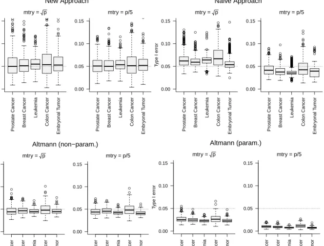
Figure 5: Type I error in Study I for the new testing approach (which uses the hold-out tion variable importance measure), the naive testing approach (which uses the classical permuta-tion variable importance measure) and the approach of Altmann et al. (2010) (non-parametric and

parametric). Hypothesis tests were performed at significance level α= 0.05 (dashed horizontal

line).

fulfilled for the classical and the cross-validated variable importance. This motivates the use of this novel measure in our proposed testing procedure.

3.2

Type I error

The type I errors of all approaches are investigated using Study I and are depicted in Figure 5.

The type I errors of our novel testing procedure are always close to the significance levelα= 0.05,

indicating that the test does not systematically reject the null hypothesis too often or too rare.

Our studies with a subset of p = 100 give similar results (Figure B.10). These findings are in

line with the results in Section 3.1.1 where it was shown that the null distribution of the hold-out variable importance is nearly symmetric around zero.

The results for the naive approach are also in line with the findings from Section 3.1.1. As expected, the type I error of the naive approach is systematically different from 0.05. More

(19)

precisely, in the studies with large predictor numbers the naive approach always gives slightly too

large type I errors if mtry is set to the default value, and too small type I errors if mtry is p₅

(Figure 5). In the studies with a smaller predictor number (p= 100), the type I errors are always

close to 0.1 for both large and smallmtry values (Figure B.10). Therefore the naive approach

should only be used with caution.

The non-parametric approach of Altmann et al. (2010) always gives type I errors close to 0.05

for both the studies with large and smaller (p = 100) predictor numbers. The type I error for

the parametric approach of Altmann et al. (2010) is always considerably smaller than 0.05 in the studies with large predictor numbers, indicating that the parametric approach is too conservative

in settings with large predictor numbers. In our studies withp= 100, in contrast, the type I error

is much closer to 0.05. The variability in type I errors was smaller for the approach of Altmann et al. (2010) than for the novel and the naive testing procedures. In settings with the predictor

space reduced top= 100 the variability increased for all testing approaches.

3.3

Statistical power

3.3.1 Study III

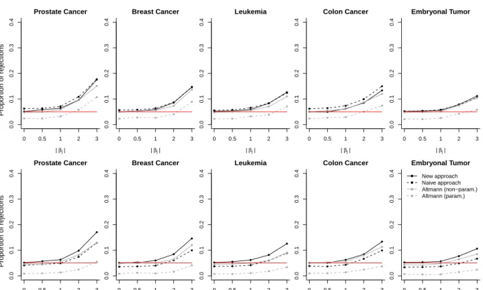
Figure 6 shows the proportion of variables withp-value below 0.05 averaged over 500 (200 for the

approach of Altmann et al. (2010), resp.) repetitions of Study III when the full predictor space is used. The proportions are computed among variables with the same absolute effect size of 0.5,

1, 2 and 3, respectively. In addition, the proportion of variables withp-value below 0.05 among

variables without effect (i.e., those variables Xj for which βj = 0) are shown. For all testing

procedures the proportion of variables withp-value below 0.05 increases with increasing absolute

effect size. Variables with larger effects are more easily identified than variables with small effects. The parametric approach of Altmann et al. (2010) consistently has the smallest power. The non-parametric approach of Altmann et al. (2010) and the new and the naive testing approaches have similar performance. However, the novel approach has slightly higher statistical power than the

non-parametric approach of Altmann et al. (2010), especially in settings withmtry=p₅. Formtry

=√pthe naive approach has a slightly higher number of variables with p-value below 0.05 than

the other two approaches for both, non-relevant (i.e.,βj= 0) and relevant (i.e.,βj 6= 0) variables.

In contrast, formtry= p₅ the naive approach has fewer variables withp-value below 0.05.

The results are in line with the results in Section 3.2, where it was shown that the type I error is smallest for the non-parametric approach of Altmann et al. (2010), and is higher (lower) for

the naive approach than for the novel approach ifmtry was set to the default value,√p(a large

value, p₅). To conclude, the novel testing approach has the best performance in the settings with

large numbers of predictor variables because it consistently has the highest power while preserving the type I error. However, the statistical power of all testing procedures was low. In our studies

with a subset ofp = 100 predictor variables, we observed much higher statistical power for all

approaches (Figure 7). The naive approach does not preserve the type I error in the settings with reduced predictor space. This can be seen when inspecting the proportion of rejections among

predictor variablesXj with βj = 0 in Figure 7. The same can be seen from the results of Study

I (Figure B.10). The novel testing approach has similar – and on average even slightly higher – statistical power than the non-parametric and parametric approaches of Altmann et al. (2010).

Note that the results presented so far are averaged over all repetitions of Study III. Thus there is no information on the variability in the selected number of variables with effect. Further

(20)

Study III – full predictor space ● ● ● ● ● 0.0 0.1 0.2 0.3 0.4 Prostate Cancer | βj| ● ● ● ● ● ● ● ● ● ● ● ● ● ● ● 0 0.5 1 2 3 ● ● ● ● ● 0.0 0.1 0.2 0.3 0.4 Breast Cancer | βj| ● ● ● ● ● ● ● ● ● ● ● ● ● ● ● 0 0.5 1 2 3 ● ● ● ● ● 0.0 0.1 0.2 0.3 0.4 Leukemia | βj| ● ● ● ● ● ● ● ● ● ● ● ● ● ● ● 0 0.5 1 2 3 ● ● ● ● ● 0.0 0.1 0.2 0.3 0.4 Colon Cancer | βj| ● ● ● ● ● ● ● ● ● ● ● ● ● ● ● 0 0.5 1 2 3 ● ● ● ● ● 0.0 0.1 0.2 0.3 0.4 Embryonal Tumor | βj| ● ● ● ● ● ● ● ● ● ● ● ● ● ● ● 0 0.5 1 2 3 Propor tion of rejections mtr y = p ● ● ● ● ● 0.0 0.1 0.2 0.3 0.4 Prostate Cancer | βj| ● ● ● ● ● ● ● ● ● ● ● ● ● ● ● 0 0.5 1 2 3 ● ● ● ● ● 0.0 0.1 0.2 0.3 0.4 Breast Cancer | βj| ● ● ● ● ● ● ● ● ● ● ● ● ● ● ● 0 0.5 1 2 3 ● ● ● ● ● 0.0 0.1 0.2 0.3 0.4 Leukemia | βj| ● ● ● ● ● ● ● ● ● ● ● ● ● ● ● 0 0.5 1 2 3 ● ● ● ● ● 0.0 0.1 0.2 0.3 0.4 Colon Cancer | βj| ● ● ● ● ● ● ● ● ● ● ● ● ● ● ● 0 0.5 1 2 3 ● ● ● ● ● 0.0 0.1 0.2 0.3 0.4 Embryonal Tumor | βj| ● ● ● ● ● ● ● ● ● ● ● ● ● ● ● 0 0.5 1 2 3 ● ● ● ● New approach Naive approach Altmann (non−param.) Altmann (param.) Propor tion of rejections mtr y = p/5

Figure 6: Proportion of rejected null hypothesis among predictor variables Xj with specified

absolute effect size_|βj| ∈ {0,0.5,1,2,3}. The mean proportions over 500 (200 for the approach of

Altmann et al. (2010), resp.) repetitions of Study III are shown when using our novel approach,

the naive approach and the approach of Altmann et al. (2010), withmtryset to√p(upper panel)

(21)

Study III – reduced predictor space ● ● ● ● ● 0.0 0.2 0.4 0.6 0.8 Prostate Cancer | βj| ● ● ● ● ● ● ● ● ● ● ● ● ● ● ● 0 0.5 1 2 3 ● ● ● ● ● 0.0 0.2 0.4 0.6 0.8 Breast Cancer | βj| ● ● ● ● ● ● ● ● ● ● ● ● ● ● ● 0 0.5 1 2 3 ● ● ● ● ● 0.0 0.2 0.4 0.6 0.8 Leukemia | βj| ● ● ● ● ● ● ● ● ● ● ● ● ● ● ● 0 0.5 1 2 3 ● ● ● ● ● 0.0 0.2 0.4 0.6 0.8 Colon Cancer | βj| ● ● ● ● ● ● ● ● ● ● ● ● ● ● ● 0 0.5 1 2 3 ● ● ● ● ● 0.0 0.2 0.4 0.6 0.8 Embryonal Tumor | βj| ● ● ● ● ● ● ● ● ● ● ● ● ● ● ● 0 0.5 1 2 3 Propor tion of rejections mtr y = 100 ● ● ● ● ● 0.0 0.2 0.4 0.6 0.8 Prostate Cancer | βj| ● ● ● ● ● ● ● ● ● ● ● ● ● ● ● 0 0.5 1 2 3 ● ● ● ● ● 0.0 0.2 0.4 0.6 0.8 Breast Cancer | βj| ● ● ● ● ● ● ● ● ● ● ● ● ● ● ● 0 0.5 1 2 3 ● ● ● ● ● 0.0 0.2 0.4 0.6 0.8 Leukemia | βj| ● ● ● ● ● ● ● ● ● ● ● ● ● ● ● 0 0.5 1 2 3 ● ● ● ● ● 0.0 0.2 0.4 0.6 0.8 Colon Cancer | βj| ● ● ● ● ● ● ● ● ● ● ● ● ● ● ● 0 0.5 1 2 3 ● ● ● ● ● 0.0 0.2 0.4 0.6 0.8 Embryonal Tumor | βj| ● ● ● ● ● ● ● ● ● ● ● ● ● ● ● 0 0.5 1 2 3 ● ● ● ● New approach Naive approach Altmann (non−param.) Altmann (param.) Propor tion of rejections mtr y = 100/5

and p₅ (lower panel). The red dashed line represents the 5% significance level.

inspection reveals, however, that the variabilities for the naive approach, the novel approach and the non-parametric approach of Altmann et al. (2010) are similar (see Figures B.4 - B.18 and Figures B.14 - B.18). The variability for the parametric approach of Altmann et al. (2010), in contrast, is smaller, which is due to the fact that the approach is very conservative and selects only few variables.

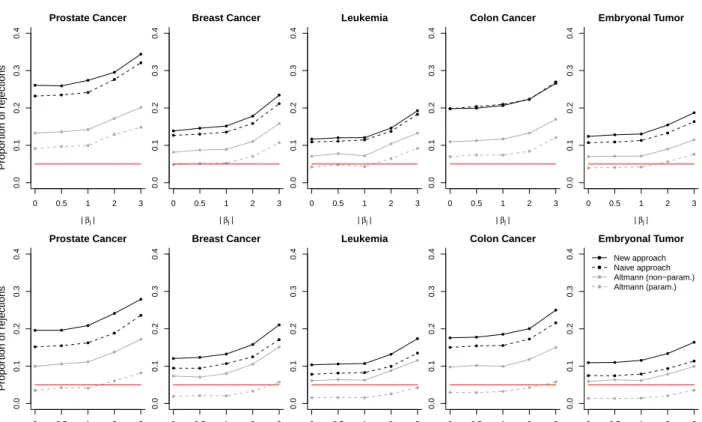
3.3.2 Study II

The results for Study II are shown in Figure 8. The proportion of variables withp-value below

0.05 is largest when using the novel testing approach. Thereafter, the proportion decreases bit by bit for the naive testing approach, the non-parametric approach of Altmann et al. (2010) and the parametric approach of Altmann et al. (2010). The approaches of Altmann et al. (2010) identify far less variables as significant than the naive and the novel testing procedures. With the

parametric approach, the proportion of variables withp-value below 0.05 is very low, especially if

mtryis set to√p. It is even lower than 0.05, indicating that the parametric approach of Altmann

et al. (2010) is too conservative. This is not the case for the non-parametric approach of Altmann et al. (2010).

In many settings the proportion of identified variablesXj withβj= 0 is very large and greatly

(22)

Study II – full predictor space ● ● ● ● ● 0.0 0.1 0.2 0.3 0.4 Prostate Cancer | βj| ● ● ● ● ● ● ● ● ● ● ● ● ● ● ● 0 0.5 1 2 3 ● ● ● ● ● 0.0 0.1 0.2 0.3 0.4 Breast Cancer | βj| ● ● ● ● ● ● ● ● ● ● ● ● ● ● ● 0 0.5 1 2 3 ● ● ● ● ● 0.0 0.1 0.2 0.3 0.4 Leukemia | βj| ● ● ● ● ● ● ● ● ● ● ● ● ● ● ● 0 0.5 1 2 3 ● ● ● ● ● 0.0 0.1 0.2 0.3 0.4 Colon Cancer | βj| ● ● ● ● ● ● ● ● ● ● ● ● ● ● ● 0 0.5 1 2 3 ● ● ● ● ● 0.0 0.1 0.2 0.3 0.4 Embryonal Tumor | βj| ● ● ● ● ● ● ● ● ● ● ● ● ● ● ● 0 0.5 1 2 3 Propor tion of rejections mtr y = p ● ● ● ● ● 0.0 0.1 0.2 0.3 0.4 Prostate Cancer | βj| ● ● ● ● ● ● ● ● ● ● ● ● ● ● ● 0 0.5 1 2 3 ● ● ● ● ● 0.0 0.1 0.2 0.3 0.4 Breast Cancer | βj| ● ● ● ● ● ● ● ● ● ● ● ● ● ● ● 0 0.5 1 2 3 ● ● ● ● ● 0.0 0.1 0.2 0.3 0.4 Leukemia | βj| ● ● ● ● ● ● ● ● ● ● ● ● ● ● ● 0 0.5 1 2 3 ● ● ● ● ● 0.0 0.1 0.2 0.3 0.4 Colon Cancer | βj| ● ● ● ● ● ● ● ● ● ● ● ● ● ● ● 0 0.5 1 2 3 ● ● ● ● ● 0.0 0.1 0.2 0.3 0.4 Embryonal Tumor | βj| ● ● ● ● ● ● ● ● ● ● ● ● ● ● ● 0 0.5 1 2 3 ● ● ● ● New approach Naive approach Altmann (non−param.) Altmann (param.) Propor tion of rejections mtr y = p/5

(23)

of the naive and the novel testing approach, variables which do not have an “own” effect, but are correlated to variables with effect, may be considered as relevant as long as they improve the trees’ prediction accuracy. Therefore, even variables that do not have a direct influence are very often identified by the two procedures – but still not as often as variables with direct influence. In contrast to that, it is not clear if the approach of Altmann et al. (2010) is also supposed to select variables that do not have a direct influence but correlate with variables that have an effect. Therefore in settings with correlated predictor variables it is not possible to evaluate which testing approach has better performance.

Note that we expect that, when based on the conditional importance of Strobl et al. (2008), the testing procedures would not as often select variables that are only associated with the response through their correlation to truly influential variables.

4

Discussion

During the last years, several approaches have been developed for hypothesis testing based on random forest’s variable importance (see Hapfelmeier and Ulm; 2013, and references therein). The existing approaches are computationally demanding and require the repeated computation of forests. In this paper we presented a fast implementation of a variable importance test that tests if a predictor variable significantly improves the forest’s predictive ability. In all our studies the novel testing procedure preserved the type I error and successfully identified at least as many relevant predictor variables as the testing approach of Altmann et al. (2010). However, our studies were restricted to classification tasks. Further studies are needed to assess if the novel variable importance test can also be applied to settings with numeric response.

Our testing procedure is based on a slightly modified version of the permutation variable impor-tance, whose null distribution was shown to be symmetric around zero. The classical permutation variable importance, in contrast, has a skewed null distribution and thus seems inappropriate for the application of our testing procedure. In our studies the testing approach based on the classical permutation importance worked quite well for settings with huge predictor numbers, but

did not preserve the type I error in settings with fewer (p= 100) predictor variables. Thus it

should be used with caution. We therefore strongly recommend the use of our testing procedure, which is based on a modified version of the permutation variable importance. This approach has consistently been shown to precisely preserve the type I error in our studies.

Our testing procedure focuses on the identification of predictor variables which significantly improve the forest’s predictive ability. The permutation variable importance measure, by its defi-nition, reflects the improvement in predictive ability if a variable is used for making the prediction.

Thus there is a monotone relationship between the value of the variable importance and the p

-value derived from our testing approach: predictor variables with higher importance scores obtain

smallerp-values. This must not necessarily be the case with permutation-based approaches. This

is obvious as Altmann et al. (2010) state that their approach corrects for the bias in the Gini impor-tance measure which ranks, for example, variables with many categories higher than variables with

fewer categories. In this case a re-sorting of variables occurs when computingp-values from the

Gini importance based on the proposed permutation procedure. If using a parametric distribution for the variable importance of unrelated variables, the permutation-based heuristic approach of Altmann et al. (2010) was very conservative in our studies and had much smaller statistical power

(24)

distributional assumptions, the testing approach of Altmann et al. (2010) showed almost the same statistical power as the novel approach. This suggests that the poor performance is related to the assumed parametric distribution for the importance scores of unrelated variables. In our studies we used the normal distribution for modeling the variable importance distribution of unrelated variables. Studies indicate that the assumption of a normal distribution is not reasonable due to the skewness of the distribution of null importance scores (data not shown). Researchers who apply the approach of Altmann et al. (2010) to high-dimensional data should therefore consider alternative distributions or approximate the null distribution in a non-parametric way.

Overall, the statistical power of all testing procedures was low in our studies with huge predictor numbers. The power of the variable importance measure to discriminate between relevant and non-relevant variables was poor, too. The approach of Altmann et al. (2010), which showed high power in other studies (Molinaro et al.; 2011; Hapfelmeier and Ulm; 2013), also had very low statistical power in our studies. This discrepancy is likely related to the fact that the existing studies included only a few variables, while our studies are based on several thousands of variables. Molinaro et al. (2011) for example focused on candidate-gene studies and considered only a few dozens of the features. When repeating our studies with a subset of 100 variables the statistical power substantially increased, and the variable importance discriminated much better between relevant and non-relevant variables. This suggests that the issue of detecting relevant features by variable importance measures is much more difficult for genome-wide association studies, including hundreds of thousands to millions of features, than for candidate-gene studies, that include only a few hundreds of features.

The novel testing approach is, however, not applicable to any high-dimensional data set. We expect that it may perform poorly if only a few non-positive importance scores are observed. If there are only a few variables with negative importance score or importance score of zero, the approximation of the variable importance null distribution might be too imprecise and might lead

to inaccurate p-values. In the most extreme setting (100 predictor variables in total and

corre-lations between predictor variables), we observed on average about 70 non-positive importance scores (for the Prostate Cancer data even only 40). However, our approach still worked surpris-ingly well. Nevertheless, in settings (i) with small predictor numbers (below 200), or (ii) with very strong correlations between predictor variables, or (iii) with high expected signal-to-noise ratio, we recommend that users look closely at the number of non-positive importance scores. If this number is small, we recommend that users be careful when using our testing approach because

it is not clear if a small number of non-positive importance scores is sufficient to derivep-values.

In such cases one should consider the computationally mo