An ACO algorithm for image compression
Cristian MartinezUniversity of Buenos Aires, Department of Computer Science Buenos Aires, Argentina, C1428EGA
E-mail: [email protected] ∗
October 29, 2006
Abstract
This paper is an application of Ant Colony Metaheuristic (ACO) to the problem of image fractal compression using IFS. An ACO hybrid algorithm is proposed for image fractal compression and the results obtained are shown. According to the tests carried out, the proposed algorithm offers images with similar quality to that obtained with a deterministic method, in about 34% less time. Keywords: Algorithms, Image Compression, Fractals, Metaheuristics
1
Introduction
For over 15 years, data compression has had relevance due to the increasing volume of personal and professional information (documents, videos, audio, images) that we use everyday. Data compres-sion software is constantly used to store or transmit information with methods that try to reduce redundant information in data file content and thus, to minimize their physical space.
Image fractal compression is among data compression methods. Defines in [11] as an image that can be completely determined by a mathematical algorithm in its thinnest texture and detail, it can then be inferred that fractal compression consists in obtaining an approximation of a real im-age by means of a set of mathematical transformations applied to certain blocks in the imim-age. A restriction on these methods is the high computational cost of image compression.
An analogy with the real ants’ behavior was presented as a new paradigm called Ant Colony Op-timization (ACO). The main features of ACO are the fast search of good solutions, parallel work and use of heuristic information, among others. Several problems have been solved using ACO: TSP, Knapsack, Cutting Stock, Graph Coloring, Job Shop, etc.
This paper proposes an ACO hybrid algorithm for image fractal compression, a problem still un-solved with ACO. In section 2, we describe some theoretical aspects of both fractal compression
and ACO. In section 3, the proposed algorithm and its variations with regard to ACO algorithms is detailed. In section 4, we show results from different tests, using varying parameter values in the proposed algorithm and comparing them to those in a deterministic one. Finally, in section 5, we suggest some aspects to bear in mind in ACO algorithm implementation based on our experience as well as possible improvements to the proposed one.
2
Fractal Compression and Ant Colony
2.1 Fractal Compression
Storing an image, for example, that of a fern in the form of pixel collection, takes up a lot of memory space - about 256 Kb. for an image of 256*256 pixels- if good resolution is required. Nevertheless, it is possible to store a collection of numbers that defines certain transformations capable of generating the fern image, but occupying 4 Kb in memory at the most. If a collection of transformations is capable of generating this for a given image, then the image can be represented in a compact way. Fractal compression describes the scheme to obtain such collection. For more details, see [7].
Suppose that we have an image I that we want to compress. We are looking for a collection of transformationsw1, w2, . . . , wn such thatW =Swi and I =|W |, i.e.
I =W(I) =
n
[
i=1
wi(I) (1)
To achieve this, image I must be broken up into blocks so that the original image is obtained when applying transformations. However, there are images that are not made up of blocks that might be easily transformed to obtain I. But an approximation I0 =|W | where the distance d(I, I’) is the smallest possible to be obtained, i.e. what is needed is to minimize the distance between original image blocks and the transformed blocks, i.e.:
M in d(I\(Ri×I), wi(I)) ∀i= 1. . . n (2)
Thus, domain blocksDi andwi transformations have to be found in order to be as close as possible
to an image blockRi (also called region) after applying a transformation to a domain block
Some definitions are given below:
• A transformation w in the n-dimensional real space Rn is a function Rn → Rn. An affine
transformation w:Rn→Rn can be written:
w(x) =Ax+b= a11 a12 . . . a1n a21 a22 . . . a2n . . . . . . . . . . an1 an2 . . . ann x1 x2 . . . xn + b1 b2 . . . bn (3)
Where A, an n-order matrix in Rn×n is called deformation matrix1 of w and vector b in Rn,
is called the traslation vector of w.
• An affine transformation w, is contractive ifkAk<1. If there is 0≤s≤1, so thatkAk< s, s being the contraction factor for the transformation w.
• Let Rn be the vectorial space with a metric d (also called distance function), An Iterated
Function System(IFS) in this space is a set of finite contractive transformations, W =
{w1, w2, . . . wm}. The contraction factor s is defined as the maximum of the contraction
factors in the transformations s = max{k w1 k,k w2 k, . . . ,k wm k}. An IFS defines its
associated transformation on the space of compact subsetsD(Rn) by W(I) =Sw
i(I) for all I ∈D(Rn).
• Given an IFS {w1, w2, . . . wm} there is a unique invariant set I so that I =Smi=1wi(I). I is the attractor of w.
• Given a metric d on n-dimensional space Rn, two sets A, B ∈ Rn, the distance between A
and B can be expressed as:
d(A, B) =max{supx∈A{infy∈Bd(x, y)}, supy∈B{infx∈Ad(x, y)}} (4)
This distance function is called Hausdorff metric of d.
• To know how to approximate an IFS attractor to an image, we use the Collage Theorem. Let W = {w1, w2, . . . , wm} be an IFS with contraction factor s, W : D(Rn) → D(Rn) its
associated transformation andA ∈D(Rn) the attractor of W. Thend(L, A)≤ d(L,W(L)) 1−s for
all L ∈ D(Rn). Therefore, the problem of searching an attractor A close to an image I is
equivalent to minimizing the distanced(I,Smi=1wi(I)). 2.2 Fractal Compression Deterministic Algorithm
This algorithm was proposed by Barnsley [1]. It divides the image into a grid of non-overlapping range blocks R ={Ri} and domain blocks D ={Di} in which partial overlapping can exist. For each range block Ri, the algorithm performs an exhaustive search over domain blocks, until a
domain block Dj is found so that the distance d= (Ri, wijk(Dj)) is minimal. Then it saves the
coordinates of Dj and the type of transformation applied. The algorithm is shown in Figure 1.
A characteristic of fractal compression is that the decompression resolution is independent of image size, so that the chosen size for decompression can be different from the size of the original image, without changing the resolution.
2.3 ACO
Ant colonies are distributive systems that form highly structured social organizations allowing them to perform complex tasks that in certain cases, exceed the individual capacities of a single agent ([2]), as in the case of food search. Basically, ants go out of the nest to look for food leaving a trace on the ground, called pheromone. In case the path chosen by an ant is shorter (in terms of time or some other measurement) than that of the rest of the ants, it would be able to deposit the food
Procedure Exhaustive(#img, #dom, #transf, R, D) list=[]
For i=0 to #img-1 list[i]=[]
min=∞
For j=0 to #dom-1 For k=0 to #transf-1
dist=distance(R[i],w(k,D[j])) if dist<min then
min=dist, dj=j, wi=k list[i]=[dj,wi]
Returnlist
Figure 1: Exhaustive algorithm
in the nest and return to look for more, thus increasing the pheromone on its path, causing other ants to follow the same path as a result of the high level of pheromone on the ground.
ACO algorithms used for solving optimization problems were developed based on the observation of the ant behavior described above. One of the most best-known ACO algorithms, is Ant System(AS). It was created in 1992 by Marco Dorigo and used to solve the TSP, based exactly on the fact that ants find the shortest path to go from the nest to the food source.
2.3.1 AS-ACO
Some details of AS-ACO algorithm that adapt actual ant behavior to minimal cost graph are shown below associating a variable τij called the artificial pheromone trace to every edge(i,j) of graph
G=(V, E). As already mentioned, ants follow the pheromone trace. The amount of pheromone deposited on each edge is proportional to the utility achieved.
Every ant constructs a step-wise solution to the problem. At each node, the ant uses the stored local information to decide the node to reach next.
When an ant k is in node i it uses the pheromone traceτij left on edges and heuristic information,
to choose j as the next node, according to the random proportional rule:
pkij = τα ijη β ij P l∈N ki τ α ilη β il if j∈ Nk i 0 if j /∈Nk i (5) beingNk
i the ant k neighborhood, in node i.
The node i neighborhood comprises all the nodes connected directly to it in the graph G=(V, E), except its predecessor to avoid returning to previously visited nodes.
Applying decision rule at each node, ant k will eventually reach the final node. Once ant k has completed its path, it deposits an amount of pheromone on the edges visited given by the following equation:
Thus, when the other ants are in node i, they will be more likely to choose node j as their next one due to higher concentration of the pheromone. An important aspect is the value that ∆τk takes.
In general, the amount of pheromone deposited is a decreasing function of path length.
Pheromone evaporation can be understood as a mechanism that allows rapid convergence of the ants towards a sub-optimum path (see [4]). In fact, decreasing pheromone favors the exploration of different paths during the search process and avoids the stagnation in local-optimum. In actual ant colonies, evaporation takes place but does not play an important role in shorter path search. The evaporation leaves behind bad decisions, and allows a continuous improvement in achieved solutions. Pheromone evaporation is applied using the following equation:
τij = (1−ρ)τij (7)
for all edges (i,j) from graph G andρ∈(0,1] a parameter of the algorithm. A general framework for the Ant Colony can be:
Procedure Ant Colony() Initialize data()
While not terminate Construct solution() Apply localsearch() Update pheromone()
Figure 2: AS-ACO Algorithm
3
Algorithmic Details
This section explains how ACO metaheuristic was adapted to image compression problems, detailing aspects related specifically to compression.
3.1 Pheromone
The success of an ACO algorithm depends, among other variables, on pheromone trace definition. This depends on the problem to be solved. For example, in the TSP solved in [3], the pheromone deposited on edge (i, j) denotes the benefits of going to city j, from city i. In the Bin Packing problem solved in [10], the pheromone deposited on edge (i, j) reflects the benefit of having items i and j in the same bin. In our work, the pheromone deposited on edge (i, j) refers to associating range block i and domain block j. The pheromone matrix is rectangular (not symmetrical) where the rows indicates range blocks (image blocks) and the columns domain blocks (blocks to transform). 3.2 Heuristic Information
The possibility of using heuristic information to direct probabilistic construction of solutions by the ants is important because it allows considering problem specific knowledge. This knowledge
can be available a priori (static problems) or at run time (dynamic problems). In static problems, the heuristic information is calculated in every run of the algorithm. Examples are the inverse of distance between cities i and j used in the TSP problem of [5] and the size of item j used in the Bin Packing Problem of [10]. The static heuristic has the advantage of being computed at every iteration of the algorithm together with the pheromone information. In the case of dynamic problems, the heuristic information depends on building partial solutions and must be calculated at each step taken by the ants.
Bear in mind that the use of heuristic information is important for an ACO algorithm and that its importance decreases if local search algorithms are used. Depending on the problem to be solved, the definition of the heuristic information will be more or less complex. In section 4, the quality of the solutions obtained by the algorithm using heuristic information and local search is analyzed. In our work several alternatives of heuristic information were tested. Using the inverse of the error obtained when using the domain block j for approximating domain block i, was found to be the best one. This heuristics has to be obtained dynamically in contrast to other problems solved with ACO, where the heuristic information is static(TSP, Bin Packing, Snapsack, Job Shop, etc); the reason for this being that the error information to approximate domain blocks is not available before the optimization process and, therefore, the exhaustive exploration of the solution space is important. Further details about other options are given in section 5.
3.3 Problem Solving
As indicated previously, ants construct feasible solutions using heuristic information and pheromone. Every ant constructs its path choosing one domain block j for every range block i. The probability that an ant k chooses one domain block j for the range block i, is given by following equation:
pkij = τα ijη β ij P l∈N ki τ α ilη β il if q < e−2×antsk J otherwise (8) where:
• ηij = err1ij and errij is the error incurred in choosing block j as being close to block i. • q is a uniform random variable [0,1). In contrast to [4], where Ant Colony System algorithm
(ACS) described uses a fixed parameter q0 that serves as threshold for choosing between a probability calculation or selecting a node in a deterministic way. In this paper we use one Simulated Annealing (SA) characteristic consisting in the selection of poor solutions using an exponential expression. In addition, it is necessary to mention that the ants we used perform different kinds of work. Good and bad ants were basically used for the construction of solutions. Expression 8, allows the choice of ”bad” blocks at the beginning of the search process. We use this option for the exploration of new solution spaces. Our local optimum scape mechanism is based on the Simulated Annealing algorithm used to solve an Assignment Problem in ([12]).
The construction of solutions thus consists in choosing a domain block j for every range block i of the image, according to the above equation.
3.4 Pheromone Update
Once all ants have constructed their paths, the pheromone level is updated by evaporation followed on the deposit of new pheromone value as indicated next:
τij =τij+ ∆τijsuper (9)
Where ∆τijsuper = 1/Csuper, and Csuper is an objective function value obtained by a ”super” ant.
The adopted criterion is similar to MAX-MIN ([4]), where a selected ant is the one that deposits pheromone in every iteration. The ACO MAX-MIN algorithm is easy to implement and it yields good results. Nevertheless, a path for a ”super” ant was generated at each iteration in this paper. This path is obtained from the best domain block and an associated transformation for each range block, which was found by the other ants. That is to say, the ants perform cooperative work so that only one ant deposits pheromone in a chosen path generated by the best selections of the ant colony.
3.5 Objective Function
In order for the proposed algorithm to achieve good solutions, an objective function that measures the quality of the solutions must be used. In [3], the objective function was the minimal cost of vehicle routing, in [5] the total minimal distance for visiting all cities, in [10] an average of bin usage. Here a similar expression for fitness as the one used in [13] was applied. It basically measures the distance between image blocks (range) and domain blocks.
The expression to minimize is: M in #imgX−1 i=0 X (x,y)∈ri [(ri(x, y)−di(x, y))−(¯ri−d¯i)]2 (10) where:
• ri(x, y) is the pixel (x,y) of range block i
• di(x, y) is the transformated pixel (x,y) of domain block i used for transforming range block ri
• r¯i is the average (in rgb) of range block i
• d¯i is the average (in rgb) of domain block i used for transforming range blockri • #domis the number of domain blocks of image
3.6 Local Search and ACO
When local search is used, ACO algorithms improve their performance. We can mention [3], where 2-OPT heuristic is applied for improvement of solutions in the routing problem and [10] that uses the Martello and Toth dominance Criterion, among others.
The reason why ACO algorithms coupled with local search algorithms provide good solutions, is that they are complementary. An ACO algorithm generally achieves intermediate quality solutions, whereas local search algorithms search in the solution neighborhood, trying to improve the solution quality further.
As regards local search algorithms, the crossover operator proposed in the genetic algorithm of [13] and a local search algorithm used in [9] can be mentioned. Nevertheless, using the above mentioned algorithms implies a high computational cost. A better alternative can be obtained by a modification of Jacquin’s algorithm [8] consisting in performing the computation prior to problem solving through the block classifications.
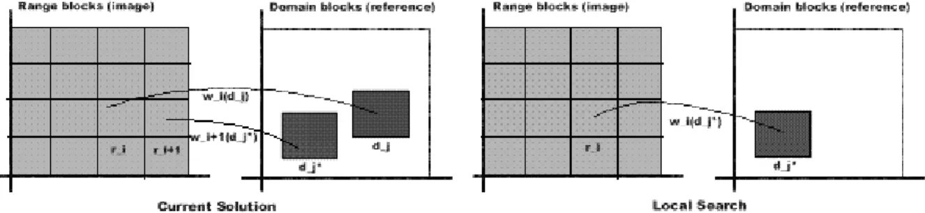
Here two local search algorithms are used.
Algorithm 1: based on the possibility of having similar blocks in images forming a region (e.g., in an tree image, surely there are zones where a group of leaves are very similar among them), given an image blockri and a domain blockdj, the algorithm compares the latter with neighboring
blocks ofri.
Figure 3, illustrates the operation of Algorithm 1.
Figure 3: Local Search Algorithm
Algorithm 2: in order to improve the quality of solutions and explore new domain blocks, for any image range block whose error in approximation is higher than the average known for the best solution so far, the algorithm assigns a random domain block even not used.
4
Computational Results
The results of some tests are commented in this section. First, the parameters of the ACO algorithm proposed will be defined and then their results will be compared with the deterministic algorithm proposed in [11]. Then the results obtained by the proposed algorithm both with and without local search will be analyzed. The experiments were done on several test images -landscapes, human faces, animals, etc.- with similar results in terms of quality and time to those reported here2. 4.1 Parameters
The parameters that will be defined correspond to our ACO algorithm:
• Number of ants: indicates the ants that will construct solutions for each iteration. According to([4]), 10 is a reasonable value. Nevertheless, other values will be considered.
• β: defines the importance of using heuristic information in contrast to pheromone information. In [4], 2 is the recommended value, in [10] 2 and 5 were used, whereas 10 and 5 were used in [5]. According to our tests, this parameter is not as relevant as the others.
• α: defines the importance of the pheromone trace. The value recommended in [4] and [10] is 1, whereas in [5] 0.1 was used. Also, it presents the same characteristic as that of β in relevancy.
• ρ: is the evaporation factor used for the control of pheromone level deposited on paths. Values close to 1 are recommended ([6], [2]).
• Stop criterion: is the number of times that the ants as a whole construct new solutions. There are others alternatives to stop execution of these algorithms, e.g. difference between two consecutive solutions, cpu time, stagnation of solutions, closeness to ideal solution, among other ones.
• Factor S: is used to obtain an initial solution. It is obtained from the sum of the product between a factor s and the difference of averages between range and domain blocks used. For the performed tests, using factors between [7,15] is recommended.
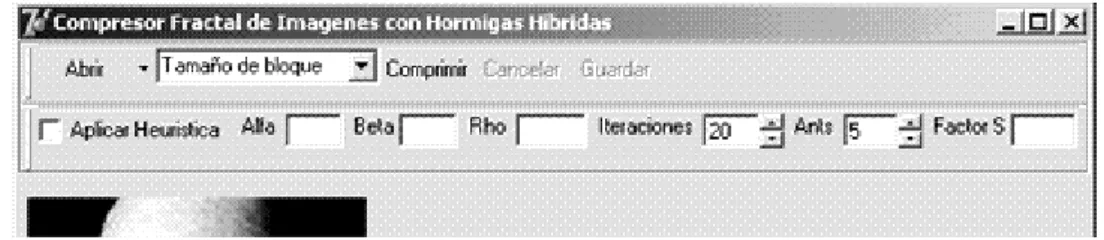
• Block size (pixels): indicates domain and range blocks size. Smaller size implies a better approximation. Based on our test results, where we evaluate time and quality, the value used is 8x8.
In Figure 5, the compressor interface is shown.
Procedure ACO Fractal(#iters,#ants,α, β, ρ, range list, domain list) Initialize data(pheromone matrix, error matrix, best solution, best obj) For i=0 to #iters-1
ant list=Construct solution(pheromone matrix,error matrix,#ants,#img,α, β) best path=Generate best path(#img,#ants, ant list, range list)
curr solution=Local search(best path, domain list,range list) Update pheromone(best solution,pheromone matrix)
curr obj=Objective(curr solution, domain list, range list) if curr obj<best obj
best obj=curr obj, best solution=best obj
Returnbest solution, best obj
Using heuristic information and pheromone, the ants build their paths in parallel. Nevertheless, the quality of solution depends on the ant position in the construction of solutions.
Procedure Construct solution(pheromone matrix,error matrix,#ants,#img,α, β) ant list=[]
For img=0 to #img-1 For k=0 to #ants-1
ifµ(0,1]< e−2#antsk
ant list[k][img]=proportional rule(img,pheromone matrix,error matrix,α, β) else
ant list[k][img]=best domain(img, pheromone matrix,error matrix,α, β)
Returnant list
Generating the best path for the ”super” ant means selecting the best domain blocks achieved by the ants.
Procedure Generate best path(#img,#ants, ant list, range list) best path=[]
For img=0 to #img-1
min error=∞, best aprox=[] For k=0 to #ants-1
curr error=error(range list[img],ant list[k][img]) if curr error<min error
min error=curr error, best aprox=ant list[k][img] best path[img]=best aprox
Returnbest path
Update pheromone consists of evaporation and deposit. Only the ”super” ant performs updates.
Procedure Update pheromone(best solution,pheromone matrix) Evaporate pheromone(pheromone matrix)
Deposite pheromone(best solution,pheromone matrix)
Figure 5: Compressor interface 4.2 Results
All tests were done in a Celeron PC 750 MHz with 256 Mb Ram, under a Windows 2000 Server. The application was developed with Delphi 6/7.
The following four tables show the results obtained (run time and objective function value obtained) for the proposed algorithm and their percentage with respect to a deterministic algorithm.
The results obtained by the deterministic algorithm are:
Objective function value:49965453 , Run time: 402 secs.
Table 1: Comparison of deterministic algorithm and ACO, using different values ofρ. Fixed Parameters
α= 1, β= 2, Iterations=45, Ants=10, Factor S=10.
ρ Time (secs) Prop. (%) Obj ∆ (%)
0.2 195 48.5 6196285 24
0.5 195 48.5 6182589 23.7
0.7 192 47.8 6178530 23.7
0.85 203 50.5 6490655 29.9
Table 1: ACO results, using different values for evaporation factor
According to Table 1, the best results correspond to evaporation factors between 0.5 and 0.7, i.e., good results with a computational time near to 50% of that used by the deterministic algorithm and objective function value within 24%.
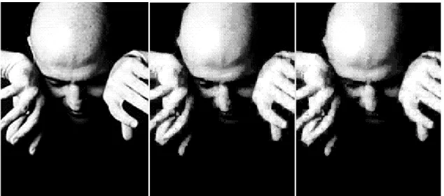
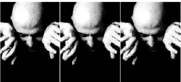
Figure 6 shows the original image, deterministic compression and our best result so far.
Table 2: Comparison of deterministic algorithm (Value: 4996545, Time: 402 secs) and ACO, using different values ofα, β.
Fixed Parameters
ρ= 0.7, Iterations=45, Ants=10, Factor S=10.
According to Table 2, the best results are obtained with α= 0.5, improving (21.9 %) with respect to Table 1. However, the execution time is higher.
Figure 6: Original image, deterministic and heuristic compression α β Time(secs) Prop. (%) Obj ∆ (%)
1 2 192 47.8 6178530 23.7 1 3.5 203 50.5 6298933 26.1 1 5 205 51 6747003 35 0.5 2 205 51 6310030 26.3 0.5 3.5 207 51.5 6090193 21.9 0.5 5 208 51.7 6211330 24.3
Table 2: ACO results, using different values for ants and iterations
Table 3: Comparison of deterministic algorithm (Value: 4996545, Time: 402 secs) and ACO, using different values for ants and iterations.
Fixed Parameters
α= 1, β= 2, ρ= 0.7, Factor S=10.
Ants Iters. Time(secs) Prop. (%) Obj ∆ (%)
10 35 161 40 6627192 32.6 10 45 192 47.8 6178530 23.7 10 55 290 72.1 6002001 20.1 15 35 217 54 6281371 25.7 5 45 139 34.5 6274252 25.6 5 55 170 42.3 6171194 23.5
According to the results obtained in Table 3, we can say that:
• Using 10 ants and 55 iterations, i.e., more iterations than the best solution obtained up to Table 2, a better solution is obtained but at the price of higher execution time (72.1 % of necessary time to obtain the deterministic value).
• Using more ants than the best solution of table 2 and fewer iterations (15 ants and 35 iterations) the results obtained do not improve over those achieved before.
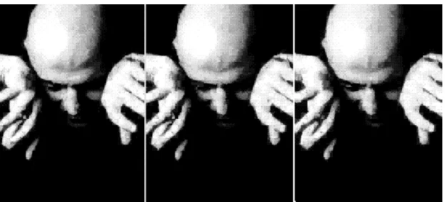
• Better execution times and quality in solutions than the best solution up to Table 2 were obtained, and they correspond to results of the last row (42.3 % of deterministic time and a variation of 23.5 % respect to the deterministic algorithm). However, there is a solution with less computation time and acceptable quality (previous to last row) shown in Figure 7.
Figure 7: Deterministic image and results of Table 1 and Table 3
As observed in Figure 7, the quality obtained with 5 ants and 45 iterations are ”acceptable” with a computational time equal to 34.5 % of the deterministic algorithm and a variation from the deterministic value of 25.6 %.
Table 4: Comparison of deterministic algorithm (Value: 4996545, Time: 402 secs) and ACO, using different values of ants and iterations, without local search algorithms.
Fixed Parameters
α= 1, β= 2, ρ= 0.7, Factor S=10.
Ants Iters. Time(secs) Prop. (%) Obj ∆ (%)
5 55 132 32.8 8984190 79.8
10 45 175 43.5 8179007 63.7
10 55 213 53 7838685 56.9
Table 4: ACO results, using different values for ants and iterations, without local search From Table 4, the best result without applying local search is higher than twice the best solution with local search (23.5 %). Also, the execution time is slightly shorter.
Figure 8 shows the deterministic result and best solutions with and without local search.
5
Conclusions
The proposal of [13] to solve the fractal compression was done using a simple objective function. The reported results shows a variation of 65 % with respect to optimal value with a computational time of 330 minutes.
In our work and in accordance with the tests performed, it is possible to obtain good-quality images with execution times close to 34 % of the deterministic time, with a variation of objective value of 25.6%. The execution time and compressed image quality allow us to state that ACO metaheuristic can be applied successfully to the fractal image compression problem. Also, our algorithm is another possible alternative for image compression.
To achieve good results, it was necessary to consider the following factors:
• Number of ants: in accordance with [4], the use of 10 (or n ants where n is in this case the number of domain blocks) is recommended. In our case, we used the first one. Bear in mind that each ant stores its path and this affects the available memory. For this reason, it is not advisable to use too many ants.
• Iterations: they depend on the problem. They are intimately related to the number of ants, and also to the number of ants that deposit pheromone. At the first stages, ”acceptable” results must be allowed as the algorithm improves the initial solution proposed. That is to say, with few iterations low-quality results are obtained.
• Evaporation factor (ρ): [6] uses 0.5 to solve the TSP problem. In this work, good results were obtained with values close to 0.7. The important thing to consider with this parameter is the fact that values near to 1 force to the exploration of new spaces of solutions while values close to 0 explore the environment of the current solution.
• Initial solution: in [2], [4] and [6] the initial pheromone applied at each edge(i, j) is done using a function that relates the number of ants with an initial solution. These works do not precise the distance this gives to the desired solution. It is important that this situation be taken into account. In this paper it is shown that the initial solution must be at most between 1.7 and 2.5 times the best value. Higher values cause a slow descent towards good solutions, while lower values can cause unfeasible solutions. Ant Colony does not need initial solutions of high quality, but it does requires them not to be too far.
• Local search: in [4] mentions the importance of the heuristic information even though it does not apply local search to the TSP problem. In this work, we mostly consider the use of local search algorithms to avoid stagnation and to ensure fast convergence to reasonable solutions. When local search was not used, the solutions obtained were far from the expected results (twice the best obtained using local search). Although this difference can be reduced, the price to pay is a bigger number of iterations causing higher execution times that not necessarily ensure reasonable solutions.
• Heuristic Information: in [3] (like most ACO proposals) considers the inverse of the distance between pairs (i, j) as heuristic information. On the other hand, [10] considers the size of items j as heuristic information. In our case, the following three alternatives were considered, being the third one the one that yielded better results:
– Difference of mean value: this alternative did not yield good results, because it was affected by extreme values. In our tests, reconstructed images had the same tonality in the whole image.
– Frequencies(i, j): it consists of saving the number of times that domain block j was used to compare with range block i. This option did not work, because it is possible that the ants choose bad domain blocks(major error) and cause the others to follow the same path and thus increase the frequency of use.
– Error of selection(i, j): as indicated previously, it is the error caused by choosing domain block j to compare with range block i. Thus, the frequencies are not considered. Also, the information is variable, not fixed as in the the majority of problems solved with ACO. Basically, the selection error is equivalent to the cost of selection.
Finally, there are several possible strategies that can be applied to improve results:
• Categorization of blocks: in [8] this is done to solve the problem in deterministic manner. Nevertheless, the time of block categorization before solving the problem must be considered. Through the categorization of blocks it is possible to obtain compressed images that are more similar to the original ones and have better compression ratios.
• Local search: to improve paths obtained by the ants using other local search algorithms.
• Cooperative work: In our work, all ants collaborate to obtain a better path. However, several types of ants can be defined each performing different tasks and collaborating to ensure better solutions.
Acknowledgments
To Irene Loiseau and Silvia Ryan for their comments and suggestionss, which helped to improve the quality of this work.
References
[1] Barnsley, M., Fractal Image Compression, A.K. Peters, 1993, pp. 89-116.
[2] Bonabeau, E., Dorigo, M. and Theraulaz,G.,Swarm Intelligence, Oxford, 1999, pp. 32-77. [3] Bullnheimer B., Hartl, R. and Strauss, C., “Applying the Ant System to the Vehicle
Rout-ing Problem”,The Second Metaheuristic International Conference, Sophia-Antipolis, France, 1997.
[4] Dorigo, M. and Stutzle, T., Ant Colony Optimization, MIT, 2004, pp. 12-117.
[5] Dorigo, M. and Gambardella, L., “Ant Colonies for the Travelling Salesman Problem”, BioSys-tems, 1997, V43, pp. 73-81.
[6] Dorigo, M., Di Caro, G. and Gambardella, L., “Ant Algorithms for Discrete Optimiza-tion”,Technical Report IRIDIA, 1998, V10.
[7] Fisher, Y., “Fractal Image Compression”, Siggraph, Course Notes, 1992.
[8] Jacquin, F., “Image Coding Based on a Fractal Theory of Iterated Contractive Image Trans-formations”,IEEE Transactions on Signal Processing, 1991, V1, pp. 18-30.
[9] Hamzaoui, R., Saupe, D. and Hiller, M., “Fast Code Enhacement with Local Search for Fractal Compression ”,Proceedings IEEE International Conference on Image Processing, 2000. [10] Levine, J. and Ducatelle, F., “Ant Colony optimization and local search for the bin packing
and cutting stock problems”, Journal of the Operational Research Society, Special Issue on Local Search, 2004, V55, N7, pp. 705-716.
[11] Lu, N., Fractal Image Compression, Academic Press, 1997, pp. 2-82.
[12] Ryan, S., Martinez, C. and Ryan, G., “Problema de Asignaci´on de Aulas en la Universidad Nacional de Salta”,Sobrapo , Minas Gerais, Brasil, 2004.
[13] Vences, L. and Rudomin, I., “Genetic Algorithms for the Fractal Image and Image Sequence Compression”,Visual 97, DF, Mexico, 1997.