Optimal Auxiliary Variable Assisted Two-Phase Sampling Designs.

MASTER’S THESIS

Department of Mathematical Sciences

Division of Mathematical Statistics

CHALMERS UNIVERSITY OF TECHNOLOGY

UNIVERSITY OF GOTHENBURG

Optimal Auxiliary Variable Assisted

Two-Phase Sampling Designs

Department of Mathematical Sciences

Division of Mathematical Statistics

Chalmers University of Technology and University of Gothenburg

SE – 412 96 Gothenburg, Sweden

Optimal Auxiliary Variable Assisted Two-Phase Sampling

Designs

Two-phase sampling is a procedure in which sampling and data collection is conducted in two phases, aiming at achieving increased precision in estimation at reduced cost. The first phase typically involves sampling a large number of elements and collecting data on variables that are easy to measure. In the second phase, a subset is sampled for which all variables of interest are observed. Utilization of the information provided by the data observed in the first phase may increase precision in estimation by optimal selection of sampling design the second phase.

This thesis deals with two-phase sampling when a random sample following some gen-eral parametric statistical model is drawn in the first phase, followed by subsampling with unequal probabilities in the second phase. The method of maximum pseudo-likelihood estimation, yielding consistent estimators under general two-phase sampling procedures, is presented. The design influence on the variance of the maximum pseudo-likelihood estimator is studied. Optimal subsampling designs under various optimality criteria are derived analytically and numerically using auxiliary variables observed in the first sam-pling phase.

Keywords: Anticipated variance; Auxiliary information in design; Maximum pseudo-likelihood estimation; Optimal designs; Poisson sampling; Two-phase sampling.

I would like to thank my supervisors, Vera Lisovskaja and Olle Nerman, for guidance during this project. I am especially grateful to Vera for sharing thoughts and ideas from your manuscripts, on which much of the material in this thesis is based.

1 Introduction 1 1.1 Background . . . 2 1.2 Purpose . . . 2 1.3 Scope . . . 3 1.4 Outline . . . 3 2 Theoretical Background 5 2.1 A General Two-Phase Sampling Framework . . . 5

2.2 Two Approaches to Statistical Inference . . . 7

2.2.1 Maximum Likelihood . . . 7

2.2.2 Survey Sampling . . . 13

2.3 Maximum Pseudo-Likelihood . . . 17

2.3.1 Topics in Related Research . . . 24

2.4 Optimal Designs . . . 26

3 Optimal Sampling Schemes under Poisson Sampling 31 3.1 The Variance of the PLE under Poisson Sampling . . . 32

3.1.1 The Total Variance . . . 32

3.1.2 The Anticipated Variance . . . 34

3.2 Optimal Two-Phase Sampling Designs . . . 37

3.2.1 L-Optimal Sampling Schemes . . . 37

3.2.2 D and E-optimal Sampling Schemes . . . 39

3.3 Some Modifications . . . 40

3.3.1 Adjusted Conditional Poisson Sampling . . . 40

3.3.2 Stratified Sampling . . . 41

3.3.3 Post-Stratification . . . 42

4 Examples 44 4.1 The Normal Distribution . . . 44

4.2 Logistic Regression . . . 53

4.2.1 A Single Continuous Explanatory Variable . . . 55

4.2.2 Auxiliary Information with Proper Design Model . . . 59

4.2.3 Auxiliary Information with Improper Design Model . . . 63

4.2.4 When the Outcome is Unknown . . . 65

5 Conclusion 66 Appendices 69 A The Variance of the Maximum Pseudo-Likelihood Estimator 69 A.1 Derivation of the Asymptotic Conditional Variance . . . 69

A.2 On the Contributions to the Realized Variance . . . 70

P Infinite target population.

S1 First phase sample, random sample from P. Elements denoted byk,l etc.

S2 Second phase sample, probability sample from S1.

Ik Sample inclusion indicator variable,Ik= 1 if k∈S2 and 0 else.

πk First order inclusion probability, πk=P(k∈S2) =P(Ik = 1).

πkl Second order inclusion probability,πkl=P(k,l∈S2) =P(Ik= 1, Il= 1).

N,|S1| Size of first phase sample.

n,|S2| (Expected) size of second phase sample. Y Outcome, response variable.

X Explanatory variable.

Z Auxiliary variable.

Yk,Xk ,Zk Study variables corresponding to element k.

y, ˜X , ˜Z Realizations of study variables.

yk,xk ,zk Realized study variables corresponding to element k.

f(yk|xk;θ) Model of interest.

θ= (θ1, . . . , θp) Parameter of interest.

f(yk,xk|zk;φ) Design model.

S(θ) =∇_θ`(θ;y,X˜) Score, gradient of log-likelihood function. ˆ

θM L Maximum likelihood estimator (MLE).

Σ_θˆ Asymptotic variance-covariance matrix of MLE. I(θ) Fisher information matrix.

`π(θ;y,X˜) Pseudo log-likelihood function. ˆ

θπ Maximum pseudo-likelihood estimator (PLE).

Sπ(θ) =∇θ`π(θ;y,X˜) π-expanded score, gradient of pseudo log-likelihood function.

e

1

Introduction

In many areas of research, data collection and statistical analysis play a central role in the acquisition of new knowledge. However, collection of data is often associated with some cost, and in studies involving human subjects possibly also with discomfort and potential harm. There are often also statistical demands on the analysis, namely that the characteristics or parameters of interest should be estimated with sufficient precision. Efficient use of data is thus tractable for economical, ethical and statistical reasons. The precision in estimation depend on the number of observations available for analysis as well as on the study design, i.e. the conditions under which the study is conducted in combination with the methods used for sample selection.

A special situation arise when some information about the elements or subjects avail-able for study is accessible prior to sampling. Incorporation of such information in design and analysis of a study can improve the precision in estimation substantially. In practice, such information is seldom available prior to study but rather obtained through a first sampling phase, collecting data of variables that are easily measured for a large number of subjects. A sampling procedure in which sampling and data collection is performed in two phases is called two-phase sampling, and could be used to meet the statistical and economical demands encountered in empirical research.

While two-phase sampling provides an opportunity to select elements that are be-lieved to contribute with much information to the analysis, it also introduces a number of challenges. It is important to use methods of estimation that properly account for the sampling procedure, and to understand how the selection of elements influence the precision in estimation of the parameters of interest. The former is necessary in order to obtain valid inferences, the latter in order to be able to use the data available in an efficient way.

1.1

Background

Two-phase sampling as a tool to achieve increased precision in estimation in studies with economical limitations was proposed by Neyman [34] within the context of survey sampling. It is a procedure in which sampling is conducted in two phases, the first involving a large sample and collection of information that is easily obtained, the second involving a smaller sample in which the variables of interest are observed. The idea is that use of easy accessible data could aid in the collection of data from more expensive sources.

The variables observed in the first phase that are called auxiliary variables. These are not necessarily of particular interest themselves, but can be used in design and analysis of a study to increase precision in estimation. It is assumed that the variables of interest are associated with a high cost, making it unfeasible to observe these for all elements in the first phase and profitable to collect other information for a large number of elements in the first phase. The high cost could for example be due to need for interviews be carried out or measurements to be made by trained staff in order to assess or measure the variables of interest. It is also assumed that the auxiliary variables are related to the variables of interest.

The use of auxiliary variables in design, estimation and analysis is well studied within the field of survey sampling, see for example S¨arndal et al. [45]. It is however less fre-quently encountered among practitioners in other statistical disciplines. The use of two-phase sampling in case-control studies has been suggested by Walker [47] and White [48], and in clinical trials by Frangakis and Baker [15]. Another possible area of application is to naturalistic driving studies, such as the recently conducted European Field Oper-ational Test (EuroFOT) study [1]. This study combines data from different sources, in-cluding video sequences continuously filmed in the drivers cabin as well as automatically measured data, such as speed, acceleration, steering wheel actions and GPS coordinates. The access to automatically generated data could possibly be used for efficient selection of video sequences for annotation and analysis.

Optimal subsampling designs using auxiliary information have previously been stud-ied in the literature, see for example Jinn et al. [27], Reilly and Pepe [38,39] and Frangakis and Baker [15]. Much of the previous work in the area is however limited in the classes of estimators and models considered.

1.2

Purpose

The aim of this thesis is to derive optimal subsampling designs for a general class of esti-mators and statistical models, using auxiliary information obtained in the first sampling phase to optimize the sampling design in the second phase.

1.3

Scope

The work is restricted to the use of auxiliary information in the design stage, using the method of maximum pseudo-likelihood for estimation. The pseudo-likelihood is closely related to the classical likelihood, with some modifications for use under general sampling designs. In its classical form, it does not incorporate auxiliary information in estimation. This thesis deals with two-phase sampling when a random sample following some general parametric model is drawn in the first phase, followed by Poisson sampling in the second phase. Poisson sampling is a sampling design in which elements are sampled independently of each other, possibly with unequal probabilities. Total independence in sampling of elements leads to important simplifications of the optimization problem, while the use of unequal probabilities allows for construction of flexible designs.

Some minor excursions from the above delimitation are made, introducing other designs or auxiliary information in estimation post hoc. Adjusted conditional Poisson designs and stratified sampling, as well as the use of auxiliary information in estimation by sampling weight adjustment, are mentioned.

1.4

Outline

This thesis is divided into five chapters, including the current one. Chapter 2 gives a general formulation of the two-phase sampling procedure and presents the framework for the situations considered in the thesis. The essentials in maximum likelihood estimation and survey sampling are described, and the method of maximum pseudo-likelihood esti-mation is presented. Some topics in optimal design theory are also covered. The aim is to present the most important topics and results in some generality without being too technical. Focus is thus on ideas and results rather than on proofs. References to some specific results are given in the text as presented, while references covering broader topics are given at the end of each paragraph under the sectionPerspective and Sources. This section also contains some historical remarks and comments on the material. Examples illustrating the theory and techniques presented is the thesis are given under the section

Illustrative Examples. Many of these concern the normal distribution. It is chosen due to its familiar form and well known properties, which enables for focus to be on the new topics. Many of the examples are also related and it might be necessary to return to previous examples for details left out.

The main results of this thesis is presented are Chapter 3, investigating the use of auxiliary information for selection of subsampling design. This chapter is restricted to certain classes of sampling designs, for which optimal sampling schemes are derived with respect to various optimality criteria. Some post hoc adjustments of design and methods for estimation are discussed.

The performance of the subsampling designs derived in Chapter 3 are illustrated by a number of examples in Chapter 4. These include estimation of parameters of the normal distribution and in logistic regression models, with various amount of information available in the design stage. Rather simple models are considered in order to ease

interpretation and understanding.

In the last chapter, limitations and practical implications of the work is discussed. Some of the theoretical material is presented in Appendix.

2

Theoretical Background

The main ideas about two-phase sampling are presented and the framework for the situ-ations considered in the thesis is described. The main principles of maximum likelihood estimation and survey sampling are described. Estimation under two-phase sampling, using the method of maximum pseudo-likelihood, is presented. Some topics in optimal design theory needed for comparison, evaluation and optimization of two-phase sampling design are discussed.

2.1

A General Two-Phase Sampling Framework

Consider a situation in which sampling from an infinite population P is conducted in two phases. In the first phase, a random sampleS1 ={e1,e2, e3, . . . , eN}of N elements is drawn from the target population. To simplify notation, letkrepresent element ekin

S1. Associated with each element is a number or random variables, namely an outcome

or response variableYk, explanatory variablesXk and auxiliary variablesZk. Statistical independence of the triplets (Yk,Xk,Zk) between elements is assumed. Let Y be the vector with elements Yk and denote by X and Z the matrices with rows Xk and Zk respectively. The role of the explanatory variables are to describe the outcome through some statistical model on which inference about the target population is based. The role of the auxiliary variables are to provide information about the response and/or the explanatory variables before these are observed, which can be used in the planning of design. It is not required thatZ is disjoint from (Y,X).

Conditional on the explanatory variables, Yk are assumed to be independent and follow some distribution law with density f(yk|xk;θ), where θ = (θ1, . . . , θp) is the

parameter of interest. The aim is to estimate θ, or possibly a subset or specific linear combination of its elements. As an example one may think of logistic regression, in whichf(yk|xk;θ) is the probability mass function of aBernoulli(pk) distributed random variable with pk = 1/(1 +e−x

T

coefficients θ=β= (β0, β1, . . . , βp) or possibly a subset or linear combination of those.

One might also be interested in the simpler situation without explanatory variables. It is then assumed that allYk are independent and identically distributed with some density

f(y;θ).

The realizations of (Y,X,Z), generated from the underlying population when draw-ing S1, are denoted byy, ˜X and ˜Z, respectively. The k-th element of y is denoted by

yk, which is the realized value of the response variable for element k in S1. Similarly,

the rows in the matrices ˜X and ˜Z corresponding to element k are denoted by xk and

zk, respectively. If measurement of some components in (y,X˜) is associated with a high cost, the need for a second sampling phase is introduced by infeasibility of observing all of (y,X˜) for all elements in S1. It is thus not possible to estimate θ from the first

sample, since the outcome or some of the explanatory variables are unknown. A second sampling phase is thus conducted.

The second phase sample, with sample size or expected sample size n, is denoted by S2. The method of sampling can be such that elements are sampled with unequal

probabilities. It turns out that the precision in estimation depend on the method of sampling, and it is desirable to find a sampling design that yields a high precision. This can be achieved by use of the auxiliary variables in the planning of design, since these introduce knowledge about (y,X˜) between the two phases of sampling. This requires some prior knowledge about the relationship between auxiliary variables and outcome and explanatory variables.

It is assumed in this thesis that a model for (Yk,Xk) conditional onZk, described by some density functionf(yk,xk|zk;φ) with parameter vectorφ, is known to some extent prior to study. This model will be referred to as the design model and its parameter as the design parameter, and the use of this model will be restricted to determination of the sampling procedure in the second phase. The design model need not be completely known and must in practice often be guessed. However, a good agreement between guessed and true model is desirable for the methods described in this thesis to be used successfully. In the case of a continuous variable Yk and no explanatory variables, the design model forYkconditional onZk could for example be a linear regression model, so thatYk|Zk ∼ N(Z_kTβ, σε). If the parameterφ= (β1, . . . , βr, σε) is known to some extent prior to study and Zk explains some of the variation in Yk, knowledge about zk gives information about the distribution ofYk. Such information can be of great importance in the choice of subsampling design in the second phase.

Once the subsampleS2is drawn, the realizations (yk,xk) are observed for the sampled elements. Estimation of θ can then be carried out from the sampled elements in the second phase sample. However, the distribution of Yk given Xk in the sample might differ from the underlying population distribution, since S2 is not necessarily a simple

random sample. The sampling procedure must be properly taken into account in the analyses in order to obtain valid inference aboutθ. One alternative is to use the method of maximum pseudo-likelihood, which is introduced in Section 2.3.

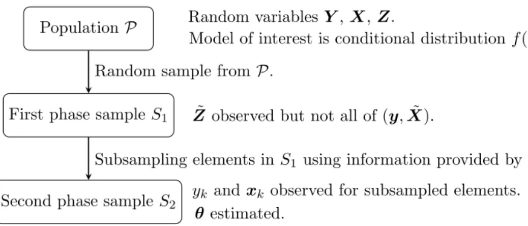
A flowchart presenting the two-phase sampling procedure is presented in Figure 2.1. The key feature in two-phase sampling is that some information about the elements in

S1is available between the two sampling phases by observation of the auxiliary variables.

Efficient use of the auxiliary information in the planning of subsampling design might improve precision in estimation.

PopulationP

First phase sample S1

Second phase sampleS2

Random sample from P.

Subsampling elements inS1 using information provided by ˜Z.

Random variablesY,X,Z.

Model of interest is conditional distributionf(y|x;θ).

˜

Z observed but not all of (y,X˜).

yk and xk observed for subsampled elements.

θ estimated.

Figure 2.1: Flowchart describing the two-phase sampling procedure.

2.2

Two Approaches to Statistical Inference

Two random processes are involved in the two-phase sampling procedure considered in this thesis. In the first phase, randomness is introduced by the distribution of (Y,X) in the underlying population, which is described by some statistical model. In the second phase, randomness is introduced by subsampling of elements inS1. This random

process is fully described by the sample selection procedure. An inference procedure that properly accounts for both sources of randomness is required and will be introduced in Chapter 2.3. Before that, two different types of inference procedures, dealing with the two random processes separately, will be discussed.

2.2.1 Maximum Likelihood

Consider a random sampleS1 of N elements from an infinite population P. Associated

with each sampled element is some variables (yk,xk), generated from some population model for which inference is to be made. Conditional on the explanatory variables, the response variables Yk are assumed to be independent and to have density f(yk|xk;θ), where θ is the parameter of interest. Estimation of θ is often carried out using the method of maximum likelihood, which now will be described.

The Maximum Likelihood Estimator

The maximum likelihood estimator (MLE) of θ, denoted by ˆθM L, is defined by ˆ

θM L:= argmax θ

where the likelihood L(θ;y,X˜) is the joint density of Y given X seen as a function of

θ. Due to independence, the likelihood function can be written as

L(θ;y,X˜) = Y k∈S1

f(yk|xk;θ) .

In place of the likelihood, it is often more convenient to work with thelog-likelihood

`(θ;y,X˜) := logL(θ;y,X˜) = X k∈S1

logf(yk|xk;θ), (2.2.1) which has the same argmax as the likelihood. The argumentk∈S1 under the sum will

be omitted from now on, simply writing sum overk.

The solution to (2.2.1) is found by solving the estimating equation ∇θ`(θ;y,X˜) =0, where ∇<sub>θ</sub>`(θ;y,X˜) = ∂`(θ;y,X˜) ∂θ1 , . . . ,∂`(θ;y,X˜) ∂θp !

is the gradient of the log-likelihood. It is often also called thescore and will be denoted by S(θ) to simplify notation. Strictly speaking, finding the global maximum of (2.2.1) requires all critical points of the log-likelihood to be considered and the boundary of the parameter space to be investigated, following standard procedures in multivariate calculus. The examples presented in this thesis will however only be concerned with finding the solutions to the estimating equation (2.2.1), leaving the additional steps to the reader for verification that a global maximum is found.

Asymptotic Properties of the MLE

The asymptotic distribution of a maximum likelihood estimator is multivariate normal

with _√

N( ˆθM L−θ)∼

a N(0,Γ) , using the notation ”∼

a” for the asymptotic distribution of a random variable. The variance-covariance matrix Γ called the asymptotic variance of the normalized MLE. The MLE is asymptotically unbiased, which we write

E( ˆθM L) =

a θ ⇔ E( ˆθM L)→θ asN → ∞, using the notation ”=

a” for equalities that hold in the limit. Furthermore, the bias of the MLE is relatively small compared to the standard error. This implies that the MLE is approximately unbiased for large samples and the bias can be neglected. Also, the MLE converge in distribution to the constant θ asN tends to infinity, and we say that the MLE is consistent. That is, the distribution of ˆθM L is tightly concentrated

around θ for large samples, so that the MLE with high certainty will be within an arbitrary small neighborhood of the true parameter if N is large enough. The MLE is alsoasymptotically efficient, which roughly speaking is to say that the MLE has minimal asymptotic variance.

Note that unbiasedness and normality of MLE is guaranteed only in the limit as the sample size tend to infinity. However, for finite samples it is reasonable to think of asymptotic equalities as large sample approximations and of to use asymptotic distribu-tions as large sample approximadistribu-tions of the sample distribution of an estimator.

The Fisher Information and the Variance of the MLE

The asymptotic distribution of the MLE can also be written as ˆ

θM L ∼

a N θ,Σθˆ

.

The variance-covariance matrix Σ_θˆ of the MLE is the inverse of the so called Fisher

information I(θ): I(θ) = EY|X " X k ∇_θlogf(Yk|xk;θ)∇Tθ logf(Yk|xk;θ) # = EY|X[−∂θS(θ)] , (2.2.2)

where∂θS(θ) =∇θ∇Tθ`(θ;y,X˜) is the Hessian of the log-likelihood. The Fisher infor-mation will also be referred to as the information matrix. The elements of (2.2.2) are given by I(θ)_(i,j)=X k E_Yk|Xk ∂logf(Yk|xk;θ) ∂θi ∂logf(θ;Yk,xk) ∂θj =X k EYk|Xk −∂ 2_logf(Y k|xk;θ) ∂θi∂θj .

Typically, the Fisher information depends on the values of the explanatory variables ˜X

as well as on the parameterθ. However, ifYkare independent and identically distributed and there are no explanatory variables, the information matrix simplifies to

I(θ)(i,j)=NEY ∂logf(Y;θ) ∂θi ∂logf(Y;θ) ∂θj =NEY −∂ 2_logf(Y;θ) ∂θi∂θj . (2.2.3)

The variance-covariance matrix can be estimated by the inverse of the estimated information matrix, which provides a simple connection between the score of and the variance of the MLE. Sinceθis unknown, the information matrix must be estimated. One possibility is simply to plug in the estimate ˆθM L instead ofθ in the Fisher information

I(θ). This estimator is referred to as theexpected information. Another commonly used estimator is

ˆ

I( ˆθM L) =−∂θS( ˆθM L) , which is called the observed information. It has elements

ˆ I( ˆθM L)(i,j)=− X k ∂2logf(yk|xk; ˆθM L) ∂θi∂θj .

Ignoring the randomness of ˆθM L, the first estimator I( ˆθM L) is the expectation of the observed information. In practice, the observed information is often preferred before the expected information [14].

Perspective and Sources

Much of the early contributions to the development of the theory of maximum likelihood estimation is due to R. A. Fisher. The main topics in maximum likelihood theory are covered by most standard textbooks in statistics, see for example Casella and Berger [9]. The asymptotic results presented in this section are quite general and holds for most standard distributions. Necessary conditions for these to hold essentially has to do with the support and differentiability of f(y|x;θ), see Casella and Berger [9] or Serfling [42] for more details on these technical conditions.

Illustrative Examples

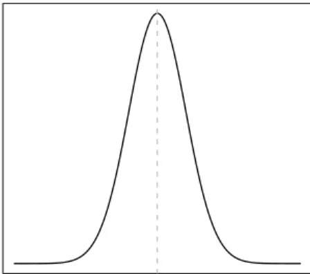
Example 2.2.1 (The Likelihood Function) Suppose that Yk are independent and

identically distributed with Yk ∼ N(µ, σ), k = 1, . . . , N, where σ is known. Given

the observed data y= (y1, . . . , yN) the likelihood is a function ofµ:

L(µ;y) =Y k f(yk;µ) = Y k 1 √ 2πσ2e −1 2 (_yk−µ)2 σ2 = 1 (2πσ2₎N/2e −1 2 P k(yk−µ)2 σ2 ,

which is illustrated in Figure 2.2. The maximum likelihood estimator µˆM L of µ is

cho-sen so that L(µ;y) is maximized, i.e., µˆM L is the point along the x-axis for which the

µ

Lik

elihood

Figure 2.2: The likelihood as function ofµfor a sample from aN(µ, σ)-distribution, where

σis known. The MLE is the point along the x-axis for which the maximum along the y-axis is reached, indicated by the grey line in the figure.

Example 2.2.2 (Estimating Parameters of the Normal Distribution) Suppose that

Yk are independent and identically distributed with Yk ∼ N(µ, σ), k = 1, . . . , N, where

both µ and σ are unknown. The maximum of L(µ, σ;y) is found by maximizing the log-likelihood `(µ, σ;y) =−N 2 log(2πσ 2₎₋ 1 2 P k(yk−µ)2 σ2 .

The partial derivatives of the log-likelihood are

∂`(µ, σ;y) ∂µ = X k yk−µ σ2 , ∂`(µ, σ;y) ∂σ =− N σ + X k (yk−µ)2 σ3 .

Solving S(µ, σ) =0 gives the maximum likelihood estimators forµ and σ as

ˆ µM L = P kyk N , ˆ σM L= r P k(yk−µˆM L)2 N .

The second order partial derivatives of logf(Y;µ, σ) are given by

∂2logf(Y;µ, σ)

∂µ2 =−

1

∂2logf(Y;µ, σ) ∂σ2 =−3 (Y −µ)2 σ4 + 1 σ2 , ∂2logf(Y;µ, σ) ∂µ∂σ =−2 Y −µ σ3 .

According to (2.2.3), the Fisher information is thus

I(θ) =N EY 1 σ2 2 Y−µ σ3 2Y_σ−3µ 3 (Y−µ)2 σ4 −_σ12 ! = N σ2 0 0 2_σN2 ! .

The information matrix has inverse

Σθ= σ2 N 0 0 ₂σ_N2 ! ,

which is the asymptotic or approximate variance-covariance matrix of(ˆµM L,σˆM L). Note

that the asymptotic distribution of the sample mean is µˆM L∼

a N(µ, σ

2_{/N), which}

coin-cide with the sample distribution of µˆM L for finite samples. Note also that (ˆµM L,σˆM L)

are asymptotically independent, which also holds for finite samples. Finally, the variance-covariance matrix of (ˆµM L,σˆM L) can be estimated by

ˆ Σ_θˆ= ˆ σ2 M L N 0 0 ˆσ 2 M L 2N ! .

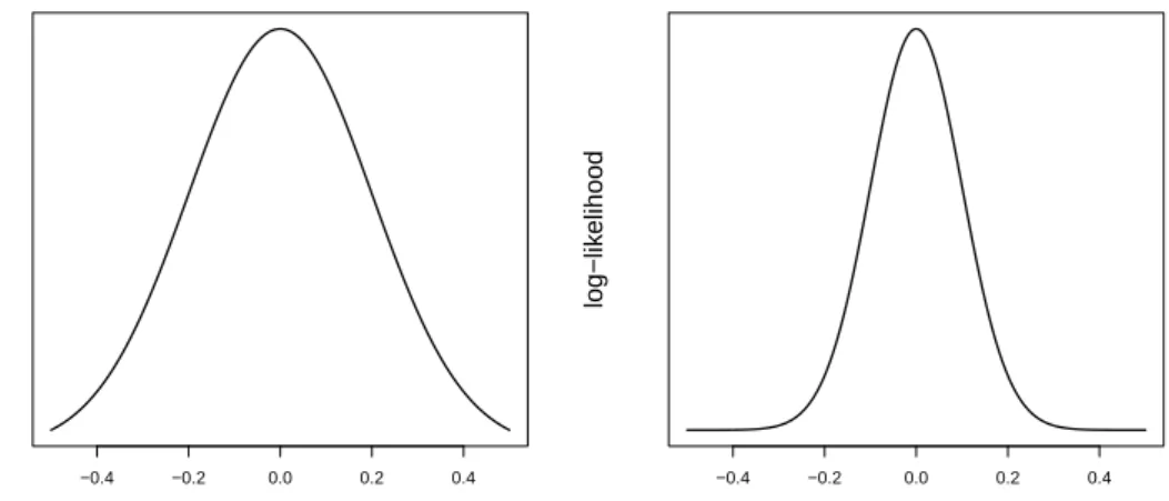
Example 2.2.3 (The Fisher Information) A simple example illustrating the con-nection between the second order derivatives of the log-likelihood and the variance of an estimator is now given.

Consider two simple random samples from a normal population with known vari-ance, the first sample being of size 25 and the second of size 100. The corresponding log-likelihoods are shown in Figure 2.3. The smaller sample has a blunt peak around the estimated value. There are thus many points that are almost equally likely given the observed data. If another sample is drawn, another value close to the current peak will probably be the most likely value. A blunt peak thus corresponds to a large variance. In terms of derivatives of the log-likelihood, this is the same as to have a small negative sec-ond derivative atθˆM L. The larger sample has peaked log-likelihood around the estimated

value and a large second derivative of the log-likelihood atθˆM L, corresponding to a small

set of estimates which are likely under the observed data and thus small variance of the estimator.

The information the sample contains about µ is summarized by the Fisher informa-tion number, which is

I(µ) =NEY ∂2logf(Y;µ) ∂µ2 = N σ2 .

The second sample has four times larger sample size and thus contain four times as much information about µ as the first sample, resulting in a variance reduction in µˆM L by a

factor 4. This example shows that increasing the sample size is one way to achieve larger information and smaller variance. It will later be shown how increased information and reduced variance can be achieved also by choice of design.

−0.4 −0.2 0.0 0.2 0.4 µ log−lik elihood −0.4 −0.2 0.0 0.2 0.4 µ log−lik elihood

Figure 2.3: The log-likelihood as function of µfor a sample from a N(µ, σ)-distribution, where σ is known. To the left: N = 25. The log-likelihood has a blunt peak around the maximum, corresponding to low information and high variance. To the right: N = 100. The log-likelihood has a tight peak around the maximum, corresponding to high information and low variance.

2.2.2 Survey Sampling

Suppose now that S1 is a fixed finite population of N elements. Associated with each

element is a non-random but unknown quantityyk. In this setting, interest could be in estimation of some characteristic of the finite population, such as the total or mean of

yk, or a ratio of two variables. By complete enumeration of all elements inS1, the actual

value of the population characteristic could be obtained. This is however often infeasible for practical and economical reasons, so a sample S2 has to be selected from which the

characteristic of interest can be estimated. Let us consider the totalt of the variableyk inS1, given by

t= X k∈S1

yk . (2.2.4) In this section, various designs for sampling from a finite population will first be dis-cussed and estimation of the total (2.2.4) will then be addressed. Even though other characteristics could be of interest, estimation of totals will be of particular interest in this thesis and other finite population characteristics will not be considered.

Sampling Designs

When drawing a sample from S1, each element in the finite population can either be

included inS2 or not, and we introduce the indicator functions

Ik=    1, ifk∈S2 0, ifk /∈S2

for the random inclusion of an element in the sampleS2. Letπk=P(k∈S2) =P(Ik= 1) be the probability that element kis included in S2, andπkl =P(k,l ∈S2) =P(Ik= 1, Il= 1) be the probability that elementkandlare both included inS2. πkand πklare referred to as the first order and second order inclusion probabilities, respectively. The inclusion probabilities are typically determined using information about the elements in the population provided by auxiliary variables known for all elements in S1.

Let I = (I1, . . . , IN) be the random vector of sample inclusion indicator functions and π = (π1, . . . , πN) be the vector of inclusion probabilities corresponding toI. Note that the indicator variables are Bernoulli(πk)-distributed random variables, possibly dependent, with

E(Ik) =πk, Var(Ik) =πk(1−πk), Cov(Ik, Il) =πkl−πkπl .

The sample selection procedure is called sampling design orsampling scheme. Of par-ticular importance are probability sampling designs. These are designs in which each element has a known and strictly positive probability of inclusion, i.e. πk > 0 for all

k∈S1.

Many different probability sampling designs are available for sampling of elements from finite populations, of which only a few will be mentioned and considered in this thesis. Broadly speaking, sampling designs can be classified as sampling with replace-ment in contrast to sampling without replacereplace-ment, as fixed size sampling in contrast to random size sampling, and as sampling with equal probabilities in contrast to sampling with unequal probabilities. Sampling without replacement is in general more efficient than sampling with replacement. Fixed size sampling designs are in general more effi-cient than sampling designs with random size. Sampling with unequal probabilities is in general more efficient that sampling with equal probabilities, if additional information is available for selection of inclusion probabilities.

Perhaps the most well known sampling design is simple random sampling, in which

n elements are selected at random with equal probabilities. A closely related sampling procedure is Bernoulli sampling, in which all Ik are independent and identically dis-tributed with πk = π. In contrast to simple random sampling, the sample size under Bernoulli sampling is random and follows aBinomial(N, π) distribution, and has expec-tation equal toN π. Independent inclusion of elements makes sampling from a Bernoulli design easy. It can be thought of as flipping of a biased coinN times, including element

A generalization of Bernoulli sampling is Poisson sampling, in which Ik are inde-pendent but not necessarily identically distributed, so that Ik∼Bernoulli(πk) withπk possible unequal. In this case the sample size is also random with expectation

E X k Ik ! =X k πk .

The random sample size follow a Poisson-Binomial distribution, which for smallπk and largeN can be approximated by a Poisson distribution, according to the Poisson limit theorem. Thinking of this in the coin flipping setting, each element has its own biased coin. Such a design is useful if one believe that some elements provide ’more information’ about the characteristic of interest than others. Another sampling procedure that makes use of this fact is stratified sampling. With this procedure, elements are grouped into disjoint groups, calledstrata, according to a covariate that explains some of the variability in y. A simple random sample is then selected from each strata. Since the covariate explains some of the variability in the variable of interest, variation will be smaller within strata than in the entire population, so that the characteristic of interest can be estimated with high precision within strata. By pooling the estimates across strata, increased precision in estimation oft can be achieved. In particular, a large gain can be achieved by choosing sampling fractions within strata so that more elements are sampled from strata with high variability iny.

The Horvitz-Thompson Estimator

Let us now consider estimation of the total (2.2.4) from a probability sample S2. A

commonly used estimator of the population total (2.2.4) is the so called π-expanded estimator, orHorvitz-Thompson estimator [24], which is

ˆ tπ = X k∈S1 Ik πk yk= X k∈S2 yk πk .

The distribution of ˆtπ over iterated sampling from S1, i.e under the distribution law of I = (I1, . . . , IN), is called the sampling distribution of ˆtπ. Note that the expectation of ˆ

tπ under the sampling distribution is E(ˆtπ) = X k E(Ik) πk yk= X k yk=t ,

provided that πk > 0 for all k ∈ S1, and we say that ˆtπ is design unbiased for t. The variance of the π-estimator is

Var(ˆtπ) = X k,l Cov Ik πk yk, Il πl yl =X k 1−πk πk y_k2+X k6=l πkl−πkπl πkπl ykyl . (2.2.5)

In similarity with estimation oft, the variance of ˆtπ can be estimated byπ-expansion as d Var(ˆtπ) = X k Ik πk 1−πk πk y_k2+X k6=l IkIl πkπl πkl−πkπl πkπl ykyl .

The above variance estimator is design unbiased provided that πkl>0 for all k,l∈S1.

The intuition behind π-expanded estimators is the following. Since fewer elements are included in S2 than in S1, expansion is needed in order to reach the total of yk in S1. As an easy example one can think of Bernoulli sampling withπk = 1/10. Since approximately 10% of the population is sampled, the total inS1will be approximately ten

times the total in the sample, and an expansion with a factor 1/πk= 10 is appropriate. In a general sampling scheme with unequal inclusion probabilities, the factor 1/πk can be thought of as the number of elements in S1 represented by element k. An element

with a high inclusion probability thus represents a small number of elements, while an element with a small inclusion probability represents a large number of elements, and the contribution of each element to the estimated total is inflated accordingly.

The use of a probability sampling design is crucial for design unbiasedness and it is easy to come up with examples with π-estimators being biased when πk = 0 for some

k. For example, think of a situation where every element withyk below the mean of yk inS1 is sampled with zero probability - this will always lead to overestimation the true

total of tinS1.

Note that inference about finite population characteristics is free of model assump-tions on the study variables, and that the statistical properties of an estimator is com-pletely determined by the design. Inference about finite population characteristics is consequently called design based, in contrast to the model based inference discussed in the previous section.

Perspective and Sources

Sample estimators for finite population characteristics rarely are unique, and optimal estimators in terms of efficiency does in general not exist [18]. It is often possible to apply more efficient estimators than the Horvitz-Thompson estimator, in particular when auxiliary information about the population is available. By incorporation of such information in estimation, substantial gain in precision can be achieved. See S¨arndal et al. [45] for a presentation of such methods, as well as for more details on the material presented in this section.

Even for inference about finite populations, the asymptotic properties of estimators could be of interest. Design based central limit theorems have been established, showing asymptotic normality and consistency oftπ and similar estimators. Important contribu-tions to the study of asymptotic properties of design based estimators have been made by H´ajek and Ros´en, among others, and the main results are covered by Fuller [17] Chapter 1.3. Since the target population is finite, any statement about the limiting be-havior of an estimator involves sequences of simultaneously increasing populations and samples, and the asymptotic properties depend on the construction of these sequences.

The requirements for convergence of sample estimators are quite technical, involving the existence of moments of the study variables and conditions on the limiting behavior of the inclusion probabilities.

Having introduced the survey sampling viewpoint on statistics, a word of clarification regarding the two-phase sampling procedure considered in this thesis might be in place. Two-phase sampling is most commonly encountered in the context of survey sampling, where the target population is a finite population. This is however quite different from the situations considered in this thesis, where the first sample is a random sample form an infinite population. The survey sampling viewpoint is to think of the study variables as fixed constants through both phases of sampling, while the viewpoint in this thesis is to think of the study variables as generated by some random process in the first phase and as constants in the second phase.

2.3

Maximum Pseudo-Likelihood

Let us now return to the two-phase sampling situation described Chapter 2.1, considering random sampling from some population model in the first phase followed by subsampling with unequal probabilities in the second phase. In contrast to the situation considered in Section 2.2.1, the conditional distribution of Yk given Xk inS2 might differ from the

underlying population distribution, sinceS2 is not necessarily a simple random sample.

Classical maximum likelihood methods can thus not be applied. However, if the log-likelihood in S1 were known, maximum likelihood could have been used to estimate θ.

Now, thinking of the first phase sampleS1as a finite population, the log-likelihood (2.2.1)

can be thought of as a finite population characteristic. Inspired the methods presented in section 2.2.2, a two-step procedure for estimation ofθ can be proposed as follows. In the first step, the log-likelihood in S1 is estimated from the observed data in S2 using

π-expansion. The second step uses classical maximum-likelihood methods to estimateθ

from the estimated log-likelihood, rather than from the log-likelihood as it appears in

S2. Doing so, the possible non-representativeness ofS2 as a sample from P is adjusted

for in the estimation procedure. This is the idea behind maximum pseudo-likelihood estimation.

The Maximum Pseudo-Likelihood Estimator

Given the observed data (yk,xk), k∈S2, obtained by any probability sampling design,

we introduce the π-expanded log-likelihood orpseudo log-likelihood as

`π(θ;y,X˜) := X k∈S1 Ik πk logf(θ;yk,xk) = X k∈S2 logf(θ;yk,xk) πk .

With maximum pseudo-likelihood estimation, themaximum pseudo-likelihood estimator

(PLE) ˆθπ chosen to be the point satisfying ˆ

θπ := argmax θ

Denote bySπ(θ) theπ-expanded score, that is the gradient of the pseudo log-likelihood. The PLE can be found by solving the estimating equation

Sπ(θ) =0 .

As for the classical MLE, a more thorough investigation of the critical points of the log-likelihood and the boundary of the parameter space than indicated above might be needed, following standard procedures in multivariate calculus.

Asymptotic Properties of the PLE

IfS2 is a probability sample, we have that

EI( ˆθπ|Y,X) = a

ˆ

θM L(Y,X) , (2.3.1) which means that the PLE is asymptotically design unbiased for the MLE conditional on the first phase sample. As the subscript indicates, expectation is taken with respect to the distribution law of I. The limiting procedure is such that |S1| = N → ∞,

|S2|= n → ∞ and n/N → h ∈ [0,1), implying also that (N −n) → ∞. That is, the

sample sizes in both phases tend to infinity, theS1grows faster thanS2but the sampling

fraction might be non-negligible.

The interpretation of (2.3.1) is as follows. ˆθM L = ˆθM L(Y,X) is a random function of (Y,X), but once the first phase sample is drawn it is determined by the realizations (y,X˜) and is no longer random. One can thus think of ˆθM L as a population parameter inS1, which is unknown since (y,X˜) are not fully observed. A subsample S2 is drawn

and ˆθM L(y,X˜) is estimated by ˆθπ = ˆθπ(y,X˜,I), which conditional on S1 is a random

function solely of I. The asymptotic equality (2.3.1) states that the mean of the PLE under iterated subsampling is approximately equal to the MLE inS1 for large samples.

One can thus think of the PLE as an estimator of the MLE, which in turn is an estimator of the population parameter. As a consequence, we have that

E( ˆθπ) = EY|X h EI( ˆθπ)|Y,X i = a EY|X( ˆθM L) =a θ ,

using the law of iterated expectation. This is to say that the PLE is an asymptotically unbiased estimator of the parameter of interest. The expectation is taken with respect to the joint distribution of (Y,X,I).

Another way to present this result is through the expression ˆ

θπ−θ= ( ˆθπ−θˆM L) + ( ˆθM L−θ) , (2.3.2) where the expectation of both terms on the right hand side are null in the limit. This follows from asymptotic unbiasedness of the PLE as an estimator of the MLE conditional onS1, and by asymptotic unbiasedness of the MLE for the population parameter. Under

some technical conditions, the bias is relatively small compared to the standard error of the estimator, and can thus be neglected for large samples. It also holds that ˆθπ is a consistent estimator of θunder the distribution of I and Y|X jointly, and that the two terms in (2.3.2) are asymptotically independent [41].

Asymptotic Normality and Variance of the PLE

Under general assumptions, the asymptotic distribution of the PLE is multivariate nor-mal with ˆ θπ ∼ a N θ,Σe_θˆ .

The variance-covariance matrixΣe_θˆ can be found using the law of total variance:

Var( ˆθπ) = VarY|X h EI( ˆθπ|Y,X) i + EY|X h VarI( ˆθπ|Y,X) i = a VarY|X[ ˆθM L(Y,X)] + EY|X h VarI( ˆθπ|Y,X) i . (2.3.3)

Using the asymptotic independence of the two terms in (2.3.2), the same result can be found directly as

Var( ˆθπ−θ) =

a Var( ˆθπ− ˆ

θM L) + Var( ˆθM L−θ) . (2.3.4) Formulas (2.3.4) and (2.3.3) show that the variance of the PLE can be decomposed into two parts, which one can think of as the variance in the first phase plus the variance in the second phase. Var( ˆθM L−θ) = VarY|X

h

ˆ

θM L(Y,X)

i

= I(θ)−1 is the variance of the MLE between first phase samples and Var( ˆθπ −θˆM L) = EY|X

h

VarI( ˆθπ|Y,X)

i

is the expectation of the conditional variance of the PLE within first phase samples. These components will be referred to as thefirst phase variance and thesecond phase variance.

Conditional on S1, the variance of the PLE around the MLE can be written as

VarI[ ˆθπ|Y,X] = a I(θ)

−1_Var

I(Sπ(θ))I(θ)−1 , (2.3.5) which is called theconditional variance. Is is obtained by a first order Taylor approxima-tion of the score [7]. A derivaapproxima-tion of the formula is given in Appendix A.1 and a simple illustration of the linearization technique is given in Example 2.3.2. The second phase variance is the expectation of the conditional variance. Putting the variance formulas together, the total variance of the PLE can be written as

Var( ˆθπ) = a I(θ)

−1_+I(θ)−1_E

Y|X(VarI[Sπ(θ)])I(θ)−1 (2.3.6)

The Design Influence on the Variance of the PLE

Let us now turn our attention to the middle term of the conditional variance (2.3.5), that is VarI(Sπ(θ)). First, we introduce the notation

s(_ki)= ∂logf(yk|xk;θ)

∂θi

,

The π-expanded score can then be written as Sπ(θ) = X k Ik πk sk .

Similar to the variance of the Horvitz-Thompson estimator (2.2.5), the design variance of Sπ(θ) has elements VarI[Sπ(θ)](i,j) = X k,l CovIk,Il Ik πk s(_ki),Il πl s(_lj) =X k 1−πk πk s(_ki)s(_kj)+X k6=l πkl−πkπl πkπl s(_ki)s(_lj) ,

in which the influence of the design on the variance of the PLE is made evident. The entire matrix can be written as

VarI[Sπ(θ)] = X k 1−πk πk sksTk + X k6=l πkl−πkπl πkπl sksTl . (2.3.7) Variance Estimation

In order to estimate the variance of the PLE, both terms in (2.3.6) must be estimated. This can be done byπ-expansion of their observed analogues evaluated at ˆθπ, that is

d Var( ˆθM L−θ) = ˆIπ( ˆθπ)−1=−∂Sπ( ˆθπ)−1 , (2.3.8) and d Var( ˆθπ−θˆM L) = ˆIπ( ˆθπ)−1   X k Ik πk 1−πk πk ˆ sksˆTk + X k6=l IkIl πkπl πkl−πkπl πkπl ˆ sksˆTl  Iˆπ( ˆθπ) −1 _, (2.3.9) where ˆsk =∇θlogf(yk|xk; ˆθπ). The estimator (2.3.8) is a π-expanded estimator of the observed Fisher information, and has elements

ˆ Iπ( ˆθπ)(i,j)=− X k Ik πk ∂2logf(yk|xk; ˆθπ) ∂θi∂θj .

The sum of the estimators (2.3.8) and (2.3.9) yield a consistent estimator of ˜Σ_θˆprovided

thatπkl>0 for allk,l∈S1, under some additional technical conditions. It is also possible

to estimate the variance of the PLE with resampling methods, such as the jackknife and bootstrap [17, 43].

Perspective and Sources

Among sampling statisticians, model based inference using pseudo-likelihood and simi-lar methods is often referred to as superpopulation modeling [21], in contrast to design based finite population modeling. Dealing with finite populations, the superpopulation viewpoint is to think of the finite population as generated from a hypothetical infinite population through some random process, and the aim of analysis is to describe the underlying random process rather than the finite population itself. The modeling con-sidered in this thesis is however not really the same as superpopulation modeling in its classical meaning, since S1 truly is a random sample.

The notion of maximum pseudo-likelihood in the context of survey sampling was introduced by Skinner [44], but the method was already present in the literature by then. Conditions under which the PLE is is consistent and asymptotically normal has been established for regression models by Fuller [16], for generalized linear models by Binder [7], for logistic regression models and proportional hazards models by Chambless and Boyle [12], and for estimators defined as solutions to estimating functions by Godambe and Thompson [19]. The subject has been treated in some more generality by Rubin and Bleuer-Kratina [41], showing consistency and asymptotic normality of estimators defined as solutions to estimating equations, such as the PLE. The asymptotic results rely on convergence of the sample estimators under the design law and of the model statistics under the model law, both converging in distribution to a normally distributed random variable. In brief, these conditions concern the existence of moments of the study variables, the continuity and differentiability of the function defining the estimating equation and some conditions pertaining to the design. In particular, the design should be such that a design based central limit theorem holds, for which the use of probability sampling is a minimum requirement.

Procedures for pseudo-likelihood estimation are available in the R package ’sur-vey’ [2, 32] and in the SAS survey procedures [25]. These software provide procedures for parameter estimation and variance estimation for most standard parametric distri-butions and models, including generalized linear models. Other software often allow for specification of element weights as an additional argument to classical maximum likelihood estimation procedures, and the PLE can then be obtained by supplying the inverse sampling probabilities 1/πk as element weights. Most such procedures are how-ever not developed for the survey sampling or two-phase sampling setting, and uses variance formulas that do not take the design and sampling procedure into account. As a consequence, the variances tend to be underestimated [5].

Much of the material presented in this section is covered by Fuller [17], Chapters 1.3, 3.3, 4 and 6. An overview of the topic is also given by Chambers and Skinner [10].

Illustrative Examples

Example 2.3.1 (The Normal Distribution) Consider a simple random sample S1

ofYk ∼N(µ, σ)with unobserved realizationsyk,k= 1, . . . , N. A subsampleS2 for which

π-expanded log-likelihood is `π(µ, σ;y) = X k Ik πk −log(2π) 2 − logσ2 2 − 1 2 (yk−µ)2 σ2 ,

with partial derivatives

∂`π(µ, σ;y) ∂µ = X k Ik πk yk−µ σ2 , ∂`π(µ, σ;y) ∂σ = X k Ik πk (yk−µ)2 σ3 − 1 σ .

The pseudo log-likelihood attains its maximum at

ˆ µπ = P k Ik πkyk P k Ik πk , ˆ σπ = v u u t P k Ik πk(yk−µˆπ) 2 P k Ik πk .

The asymptotic variance-covariance matrix of θˆπ = (ˆµπ,ˆσπ) is given by

Var( ˆθπ) = a I(θ) −1_+I(θ)−1_E Y   X k 1−πk πk sksTk + X k6=l πkl−πkπl πkπl sksTl  I(θ)−1 ,

where I(θ)−1 is given in Example 2.2.2, and

sk= Yk−µ σ2 , (Yk−µ)2 σ3 − 1 σ .

Estimation of Var( ˆθπ) can be carried out as described by (2.3.8) and (2.3.9).

Note that the maximum pseudo-likelihood estimators in the example above are of the same form as the classical maximum likelihood estimators, but with π-expansions of the term in the numerator and with the ’pseudo-sample size’ P

k Ik

πk in the denominator. Note in particular that(ˆµπ,σˆπ) = (ˆµM L,σˆM L) if S2 is a Bernoulli sample.

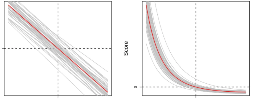
Example 2.3.2 (Variance by Linearization) A common method for deriving approx-imate variance formulas for non-linear functions of random variables is by linearization, sometimes called the δ-method. This is also the method used to derive the formula for the conditional variance (2.3.5). We illustrate this method by a simple example.

Figure 2.4 illustrates the π-expanded score as a function of µ(left) and σ (right) for a sample from a normal distribution with one known parameter. Consider first the figure to the left where the score is a function of µ and σ is assumed to be known. The thick red line is the score as function of µ in S1. If the study variable was observed for all

elements in S1, the MLE of µwould have been the point along the x-axis where the line

intersects the y-axis, in this caseµˆM L= 0. The grey lines are theπ-expanded scores for

as function of µ for 50 random subsamples from S1. For each subsample, the PLE is

the point at which the corresponding grey line intersect the y-axis. Note that the PLE varies around the MLE. The variance of the PLE around the MLE is the variance of the intersections of the grey lines with the y-axis. This is the unknown variance that we want to approximate and estimate. Note that the score is a linear function of µ, so we can write

Score(ˆµπ) =Score(ˆµM L) +b(ˆµπ−µˆM L)⇔Score(ˆµM L) =−b(ˆµπ−µˆM L) ,

since the PLE is defined to satisfy Score(ˆµπ) = 0. Taking variances on both sides, we obtain

Var [Score(ˆµM L)] =b2Var(ˆµπ−µˆM L)⇔Var(ˆµπ−µˆM L) = Var[Score(ˆµM L)]/b2 .

If we evaluate this formula at µ instead of µˆM L and insert b = I(µ), we obtain the

formula for the conditional variance given in (2.3.5).

A similar argument can also be used for the variance of σˆπ. However, the score is

not a linear function of σ so the equalities must be replaced by approximations. For samples large enough it holds thatσˆπ will be close toσ, where a linear approximation is

reasonable. µ Score 0 0 σ Score 1 0

Figure 2.4: The score as function of µ(left) and σ(right) for a sample from a N(µ, σ )-distribution illustrated a thick red line. The grey lines represent theπ-expanded scores in 50 random subsamples.

Example 2.3.3 (The Total Variance) Consider Yk ∼(µ, σ) where σ is known. The

decomposition ofVar(ˆµπ)into variance between plus variance within first phase samples

to N using simple random sampling in the second phase. When a small fraction of S1 is

subsampled almost all variance is due to sampling of elements. This variance component decreases as the sampling fraction increases and vanishes as n→N.

0.0 0.2 0.4 0.6 0.8 1.0 n/N Sim ulated V ar iance 0 Total Variance Variance Between S1 Variance Within S1

Figure 2.5: Simulated variance of ˆµπdecomposed as variance within and variance between

first phase samples based on 104 _{simulations. N = 10}3 _{observations were generated from a}

N(µ,σ)-distribution in the first phase, followed by subsampling ofnelements in the second phase. The two variance components and the total variance are plotted against the ratio

n/N.

2.3.1 Topics in Related Research

The crucial step in maximum pseudo-likelihood estimation is to obtain an unbiased estimator of the total of an estimating equation as it would have appeared in the first phase sample. This is obtained by π-expansion of the log-likelihood. This is however not the unique nor necessarily the optimal option for unbiased estimation of the log-likelihood, according to the discussion following Section 2.2.2. The PLE is in that sense not unique, and no best estimator of pseudo-likelihood type exists. Also, approximately unbiased and consistent estimators can be obtained by π-expansion of other estimating equations than the likelihood equations [44].

Criticism has been directed towards the method of maximum pseudo-likelihood for for two reasons. First, it discards the data observed in the first phase, which if incorporated in the inference procedure could lead to more efficient estimators. Second, inclusion of the sample weights 1/πk in the estimating equation often lead to large variability of the estimator. Some alternative methods for estimation and methods for improvement of the PLE have been proposed, of which a few now will be discussed.

Even though being quite similar to the MLE, the PLE does not possess all the desirable properties of maximum likelihood estimators, such as efficiency. The PLE is in general less efficient than the MLE, when the latter is valid. It is thus important to

address the question of when and why classical maximum likelihood methods cannot be applied in two-phase sampling. The notion informative and non-informative sampling designs are central concepts when dealing with this question. A sampling design is said to be non-informative if the conditional distribution of the response variable given the explanatory variables does not depend on the sampling mechanism. That is, the distribution of Y given X should be the same in S2 as in the underlying population.

Non-informative sampling implies that the sampling design is ignorable conditional on

X, and maximum likelihood inference can be carried out based onf(y|x) using the data observed in the second phase. This is related to the missing data principles of Rubin [40] and Little and Rubin [31]. If the sampling mechanism is determined by some known auxiliary variables Z, non-informative sampling can be achieved by including these as explanatory variables. However, the following three situations have been mentioned in the literature when this is not possible or suitable; when the variables used for selection of design are unavailable, when there are a large number of variables involved in the selection of design or when inclusion of these variables as explanatory variables lead to complex models, and in outcome-based designs. The latter two are relevant for the situations considered in this thesis. See Pfefferman [36,37] for a more thorough discussion about these topics.

Two main alternatives to the pseudo-likelihood under informative sampling have been proposed in the literature. Breckling et al. [8] propose a full maximum likelihood ap-proach, formulating the estimation problem as a problem of estimation under incomplete data. It is closely related to the EM-algorithm, both being based on the same missing information principle of Orchard and Woodbury [35]. In two-phase sampling, complete data is available for all elements inS2, while only the auxiliary variables are observed for

the other elements in S1. The full maximum likelihood approach makes more efficient

use of data than the pseudo-likelihood by incorporation of the auxiliary variables in es-timation. However, the full likelihood can be very complicated and might be sensitive to the model specification, involving the relations between outcome, explanatory variables and auxiliary variables.

The other proposed method is called sample likelihood and is due to Krieger and Pfeffermann et al. [30, 37]. They introduce the sample likelihood as the conditional distribution of the observed study variables given the auxiliary variables for all elements in S1. A connection between the sample likelihood and the likelihood in S1 is then

found using Bayes rule. In similarity with the full maximum likelihood, it is a model based approach to analysis and uses the first phase data more efficient than the pseudo-likelihood. It can also be extended to a Bayesian setting with prior distributions on the parameters. An overview of the methods of full maximum likelihood and sample likelihood are given by Chambers and Skinner [10] and Chambers et al. [11]. Some other methods are also discussed by Pfefferman [36].

Some improvements of pseudo-likelihood have also been proposed, addressing the variability of the PLE by modification of the sampling weights in the estimating equation. The simplest modification is to replace the sampling weights 1/πk in the estimating equation with another set of weights wk, such that known totals in S1 are estimated

correctly. This is called calibration weighting, and is well studied in the literature for sample estimators, see e.g. S¨arndal et al. [45]. Modifications of the sampling weights in the pseudo-likelihood by functions of the auxiliary variables has been proposed by Magee [33] and Kim and Skinner [28], among others.

Given the discussion above, argumentation for the use of PLE is in place. One of the major drawbacks of this method is the inefficient use of data, incorporating no in-formation about about auxiliary variables in estimation. This is however also one of the major advantages of the PLE, since the validity of the inference procedure does not rely on certain assumptions made on the auxiliary variables. The inclusion of the sam-pling weights in the estimating equation thus simultaneously protects against informative sampling and against misspecification of the often rather complex models including Z. In addition, it can quite easily be adopted to almost any kind of model and inference problem. The pseudo-likelihood might therefore be preferred due to its simplicity and general validity.

While most of the work reviewed above deals with improvement of estimators through the use of auxiliary variables in estimation, increased efficiency can also be achieved by incorporation of such information in the design. This has not been given much attention in this thesis so far, but is in fact a common feature in sampling statistics. Optimal subsampling designs in two-phase sampling has previously been addressed in the literature [15,17,27,38,39]. Much of the previous work in the area is however limited in the classes of estimators and models considered, and there is a need to address this issue in more generality. This issue will be the topic of Chapter 3.

2.4

Optimal Designs

The possibility to achieve increased precision in estimation by efficient subsampling of elements was mentioned in the previous section. In order to address this issue, a general framework for comparison of designs is needed. If estimation of a single parameter is of interest and a number of suitable designs are possible, the design giving the most precise estimate, i.e that yielding smallest variance, is often preferred. However, the notion of having ’smallest variance’ does not really have a meaning for multidimensional parameters, since the variance is not a scalar but given by a variance-covariance matrix. Still, one would like to summarize the size of the variances and covariances of all or a subset of the parameters jointly in a single number. Trying to measure the size of the variance-covariance matrix, a number ofoptimality criteria have been proposed. A few of these will now be presented and motivated geometrically.

Confidence Regions

Consider an approximately unbiased and asymptotically normal estimator ˆθ of the p -dimensional parameter θ, such as the MLE or PLE. The random variable W, defined by

W = (θ−θˆ)TΣ−_ˆ1

θ (θ− ˆ

is approximately distributed according to aχ2_p-distribution. Letχ2_p(α) denote the 1−α -percentile of theχ2_p distribution. Consider the set of pointsxsatisfying

(x−θˆ)TΣ−_ˆ1

θ (x− ˆ

θ)≤χ2_p(1−α) . (2.4.1) The set of points satisfying the above inequality defines an ellipsoid in p-dimensional space, which is called the 1−α confidence ellipsoid or 1−α confidence region forθ. It is a multivariate extension of the one-dimensional confidence interval. The confidence level or coverage probability 1−α is the approximate probability that the confidence region cover the true parameterθ. Forα sufficiently small, the confidence ellipsoid of ˆθ

will coverθ with large probability. If, in addition, the size of the confidence ellipsoid is small, ˆθ will be within a small neighborhood of θ with high probability. The precision of ˆθ is thus related to the size and shape of the confidence ellipsoid, which is what the different optimality criteria that soon will be described try to address.

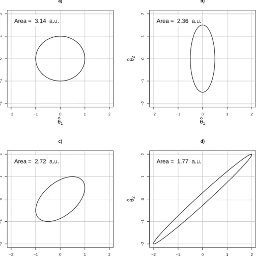
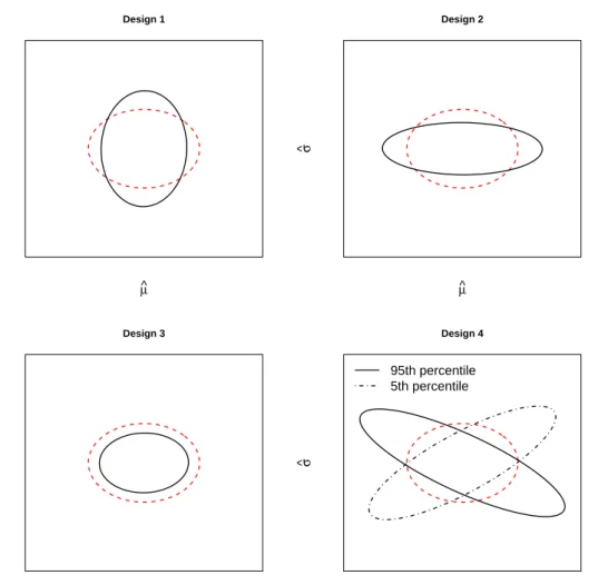
To illustrate this, the 1 −α confidence regions for a two-dimensional parameter

θ= (θ1, θ2) in four different designs are shown in Figure 2.6. Ellipses with axes parallel

to the coordinate axes correspond to designs in which ˆθ1 and ˆθ2 independent. A tilted

ellipse correspond to a design in which the estimators are correlated. The projection of an ellipse on one the coordinate axis gives us the 1−α confidence interval for the corresponding parameter. If θ1 is to be estimated with high precision, design b) is

optimal, while a) and c) are optimal with respect to the precision inθ2. The confidence

ellipsoid with minimal area is obtained with design d), but this design has the largest marginal variances along both axes. The average variance, which is proportional to the average length of the projections of the ellipses to the coordinate axes, is equal for designs a)-c) and twice as large with d). The design that minimizes the variance along the direction with maximal variance, seen as the maximal distance from the border to the center of an ellipse, is a), while the worst design in this aspect is d).

−2 −1 0 1 2 −2 −1 0 1 2 a) θ ^ 1 θ ^ 2 Area = 3.14 a.u. −2 −1 0 1 2 −2 −1 0 1 2 b) θ^ 1 θ ^ 2 Area = 2.36 a.u. −2 −1 0 1 2 −2 −1 0 1 2 c) θ ^ 1 θ ^ 2 Area = 2.72 a.u. −2 −1 0 1 2 −2 −1 0 1 2 d) θ^1 θ ^ 2 Area = 1.77 a.u.

Figure 2.6: 1−α-confidence ellipses for a two-dimensional parameter θ = (θ1, θ2). The

ellipses have different shape, orientation and area.

Optimality Criteria

As the above discussion indicate, one design is seldom optimal in all aspects. The volume, shape and axis length of the confidence ellipsoid are all important features to consider. Formula (2.4.1) shows that these properties somehow depend onΣ_θˆ. In fact, the volume

of the confidence ellipsoid is proportional to the square root of the determinant of Σ_θˆ,

denoted by det Σ_θˆ

. The design that minimizes the determinant ofΣ_θˆ, and so minimizes

the volume of the confidence ellipsoid, is calledD-optimal. The design that minimizes the average axis length, which is the same as minimizing the average variance or trace(Σ_θˆ),

is calledA-optimal. The design that minimizes the longest axis length, which is to say that minimizes the variance in the most extreme direction, is calledE-optimal. This is the same as minimizing max

|a|=1 Var(a

T_θˆ_{) = max}

|a|=1 a

T_Σ

ˆ

in Figure 2.6, design d) is the best in terms of D-optimality while a)-c) are the best in terms of A-optimality and design a) is the best in terms of E-optimality.

These three optimality criteria can also be defined in terms of the eigenvalues ofΣ_θˆ.

A variance-covariance matrix is symmetric and has thus an eigendecomposition into real orthonormal eigenvectors. The eigenvectors are orthogonal and thus correspond to independent directions and the eigenvalues are the variances along these directions, since the eigenvectors are normalized. This means that the eigenvectors are parallel to the ellipsoid axes and the eigenvalues are proportional to the length of the axes. The volume of the ellipsoid is proportional to the product of the axes lengths, and thus proportional to the product of the eigenvalues. Minimizing the volume of the ellipsoid is thus equivalent to minimizing the product of the eigenvalues of the variance-covariance matrix. Minimizing the average variance is equivalent to minimizing the average of the eigenvalues, and minimizing the variance along the direction with largest variance is equivalent to minimizing the largest eigenvalue. A summary of A, D and E-optimality criteria formulated in terms ofΣ_θˆ and its eigenvaluesλi is given below.

• A-optimality: min trace(Σ_θˆ)⇔ minPpi=1λi • D-optimality: min det Σ_θˆ

⇔ min Qp

i=1λi

• E-optimality: min max

|a|=1 a

T_Σ

ˆ

θa⇔min max_i=1,...,pλi

It is also possible to consider a subset of the parameters rather than the entire parameter vectorθ. This is useful when some components ofθ are nuisance parameters or if a specific subset of the parameters are of particular interest. A, D and E-optimality are then defined in a similar fashion on the specified subset.

Another class of optimality criteria that will be of interest in this work is linear op-timality criteria. These address the average or sum of a linear combination of elements of the variance-covariance matrix. Examples of such linear combinations are linear com-binations of variances and variances of linear comcom-binations of parameters. The former include minimizing the sum of variances, which is the same as A-optimality. L-optimality is a generalization of A-optimality in that not only variances but also covariances be-tween parameters are taken into account. A design that is optimal with respect to some linear optimality criteria is called L-optimal. Even though minimization of any linear combination of parameters ofΣ_θˆis possible, it is often of interest to consider those linear

combinations that arise from variances of linear combinations of parameters. These lin-ear combinations are of the form Var(aTθˆ) =aTΣ_θˆa. Furthermore, L-optimality allows

not only for a single such linear combination to be minimized but for the average variance over a set of linear combinations of parameters. The objective function for minimization of the average variance over m different linear combinations aT_i θˆ of estimators can be written as min m X i=1 Var(aT_i θˆ)⇔min m X i=1 aT_i Σ_θˆai .

The objective function in A-optimality in recovered by having a1 = (1,0, . . . ,0),a2 =

One property that makes D-optimality preferable before A, E and L-optimality is scale invariance. Optimal designs under A, E and L-optimality are scale dependent, and hence depend on the unit of measurement, while D-optimality is scale invariant. For this reason, D-optimality is probably the most popular optimality criteria.

Finally, it shall also be mentioned that the optimal design does also depend on the true parameter, so that different designs are optimal for different values of the true parameter.

Perspective and Sources

The methods presented in this section have a natural place in controlled experiments where the experimental settings can be chosen by the experimenter, which gives an opportunity to determine the structure variance-covariance matrix of an estimator to a large extent. The theory of optimal designs is however of importance in many other areas of application, and gives the foundation for planning of studies and experiments involving multidimensional parameters. For references regarding the material presented in this section, see Atkinson and Donev [6].