A Robust Grey Wolf-based Deep Learning for Brain
Tumour Detection in MR Images
A. Geetha1, N. Gomathi 2
1Assistant Professor, Nehru Institute of Technology
2Professor, VelTech Dr.Rangarajan Dr.Sagunthala R&D Institute of Science and Technology Avadi, Chennai, Tamil Nadu 600062
Email: geethanagaraja14@gmail.com
Abstract: In recent times, the detection of brain tumour is a common fatality in the field of the health community. Generally, the brain
tumor is an abnormal mass of tissue where the cells grow up and increase uncontrollably, apparently unregulated by mechanisms that control cells. A number of techniques have been developed so far; however, the time consumption in detecting brain tumor is still a challenge in the field of image processing. This paper intends to propose a new detection model even accurately. The model includes certain processes like Preprocessing, Segmentation, Feature Extraction and Classification. Particularly, two extreme processes like contrast enhancement and skull stripping are processed under initial phase, in the segmentation process, this paper uses Fuzzy Means Clustering (FCM) algorithm. Both Gray Level Co-occurrence Matrix (GLCM) as well as Gray-Level Run-Length Matrix (GRLM) features are extracted in feature extraction phase. Moreover, this paper uses Deep Belief Network (DBN) for classification. The DBN is integrated with the optimization approach, and hence this paper introduces the optimized DBN, for which Grey Wolf Optimization (GWO) is used here. The proposed model is termed as GW-DBN model. The proposed model compares its performance over other conventional methods in terms of Accuracy, Specificity, Sensitivity, Precision, Negative Predictive Value (NPV), F1Score and Matthews Correlation Coefficient (MCC), False negative rate (FNR), False positive rate (FPR) and False Discovery Rate (FDR), and proven the superiority of proposed work.
Keywords: Brain Tumor, Fuzzy Means Clustering Segmentation, Gray Level Co-occurrence Matrix and Gray-Level Run-Length Matrix, Grey Wolf-Deep Belief Network.
Submission: August 5, 2018 Correction: November 27, 2018 Accepted: April 28, 2019
Doi: http://dx.doi.org/10.12777/ijee.1.1.9-23
[How to cite this article: A. Geetha, N. Gomathi. (2019), A Robust Grey Wolf-based Deep Learning for Brain Tumour Detection in MR Images.
International Journal of Engineering Education, 1(1), 9-23. doi: http://dx.doi.org/10.12777/ijee.1.1.9-23]
I. INTRODUCTION
In the human being, brain plays a vital part and it is an organ controls the activities of the whole body part. Next important fact is tumor growth, and the tumor is a uncontrolled production of cancerous cells especially in any of the body part, in which the brain tumor is an uncontrolled cancerous cells’ growth in brain. The brain tumor classification is of two types: benign or malignant brain tumor[1] [9] [10]. Here, benign brain tumor has a nature of consistency structure and has no cancer cells, but in malignant brain tumor, the structure is heterogeneous and presents cancer cells. Some of the examples of benign tumors are gliomas and meningiomas, whereas some of the examples of malignant tumors are glioblastoma and astrocytomas [13].
These tumors are very dangerous as they have the ability of destroying the brain cells, and hence it damages the cells by producing inflammation, and increasing stress within the skull. Image processing
techniques are extensively used for the information extraction from the images. Image segmentation is one among them and can be described as the process of segmenting an image into non-intersecting regions [11] [14] [16]. The main goal of the classification process depends on the data types and applications. To detect an infected tumor area from the medical image, segmentation technique can be employed [12] [15] [18] [25]. Here, based on the characteristics namely contrast, color, brightness, texture, boundaries and gray levels in an image, the image can be separated into several regions. Brain tumor classification presents the separating process and classifying the tumor cells from the normal brain with the help of MR images or other medical modalities [17] [19].
If the deformity in the functioning of brain was recognized at early stage, then the brain disorders can be treated and thus can be prevented from several complications [20] [24]. There are many approaches to detect brain tumor, and most of the approaches include
diagnosing the brain tumor at the advanced stages [5] [21] [22]. Thus it is necessary to detect brain tumor at the early stage with a new technique called as Magnetic Resonance Imaging (MRI). This technique can be considered as the enhanced technique for accessing the tumor. MRI is regarded as the high resolution technique when compared with the CT and thus has no harmful effects. Even though the MRI images include several issues like intensity in-homogeneity, or dissimilar intensity ranges between the series. To eliminate these problems in MRI images, pre-processing techniques can be employed [3] [7] [23]. Thus using MRI, the internal structure of the body can be acquired in an invasive way. Thus, this technique can be very useful in medical modality for the detection of brain tumor and several other deformities. Thus it does not produce any damage to the healthy regions of the brain with its radiation during the detection process.
This paper intends develops a new detection model that includes Preprocessing, Segmentation, Feature Extraction and Classification processes. Two extreme processes such as contrast enhancement and skull stripping are processed in the initial phase; then in the segmentation process, this paper aids FCM algorithm. Both GLCM and GRLM features are extracted in the phase of feature extraction. This paper uses DBN for classification. Here, DBN is integrated with the optimization approach, and hence this paper introduces the optimized DBN, for which GWO is used here. The further arrangement of paper is as follows: Section II reviews the literature work. Section III explains the proposed brain tumour detection model. Section IV explains the developed optimized detection model. Section V explains obtained results, and Section VI ends the paper.
II. LITERATUREREVIEW Related Works
In 2017, Javeria Amin et al. [1] have developed a distinctive approach to detect and classify brain. Here, different approaches have been employed for the segmentation of applicant lesion. In this, a features set was selected for every applicant lesion with respect to shape, texture, and intensity. At that position, support vector machine (SVM) classifier was employed with various cross validations on the features set to compare the precision of proposed framework. Thus the simulation outcomes have shown that the proposed approach could attain high accuracy, sensitivity, and specificity while comparing with the other conventional approaches.
In 2015, Pawel Szwarc et al. [2] have implemented a new multi-stage automatic approach for the detection of brain and the assessment of neovasculature. Here, the symmetry of the brain was demoralized for registering the MRI series. Then the region of interest was inhibited with the tumor and peritumoral regions with respect to the intracranial structures using FLAIR (Fluid Light Attenuation Inversion Recovery) series. Furthermore, the detection of improved lesions (contrast) from the differential images has happened, and this was from either before and after the administration of contrast
medium. Lastly, there has an estimation of vascularisation that depending on the Regional Cerebral Blood Volume (RCBV) perfusion maps. Here, three types of brain tumors such as HG gliomas, metastases and meningiomas can be used for the evaluation process. From the experimental result, it was clear that the sensitivity and specificity of the contrast lesion detection were better when comparing with other manual delineation methods.
In 2015, Shang-Ling Jui et al. [3] have formulated an enhanced feature extraction approach for the improvement in the correlation among the structural deformation and the compressed brain growth. Here, a 3-dimensional inflexible registration and deformation modeling techniques were used for measuring lateral ventricular (LaV) deformation in the MRI images. Thus by verifying the locations in these extracted features, segmentation can be done using various classification techniques. Hence the proposed components were obtained with promising results with high accuracy than the other techniques.
In 2015, V. Anitha and S. Murugavalli [4] have proposed a two-tier classifier with adaptive segmentation for the classification of brain. Here, a self-organized neural network was used with the discrete wavelet transform for the extraction of features, and thus the resultant factors were then trained using K- nearest neighbor and finally the testing procedure can be done in two phases. This method classifies the brain tumor with double training process and thus gives better performance than the other existing approaches.
In 2016, Solmaz Abbasi and Farshad Tajeripour [5] have introduced a brain tumor detection automatically in 3D images. First, there performed the preprocessing work, and in this, the correction of bias field and matching histogram were employed. Next, the ‘Region of Interest’ was recognized and alienated, which was from Flair image’s background. Additionally, there employed Local binary pattern and histogram of orientation gradients as the learning features. Thus from the investigational results, it was shown that this approach was better in identifying brain tumor when comparing with the other techniques.
In 2014, Quratul Ain et al. [6] have developed a multi-stage system for the detection of brain and the extraction of regions in the brain. First, pre-processing can be done for the removal of noise in the MRI brain images. Then classification can be done for the feature extracted images using SVM classifier. After classification, the skull region was removed and extracted from the brain region. Then the separation of affected cells from the normal brain cells was done using FCM clustering. From the experimental analysis, it was clear that the region was extracted accurately with better performance.
In 2015, P. Shantha Kumar and P. Ganesh Kumar [7] have formulated an adaptive neuro-fuzzy inference system (ANFIS) with respect to a selection range that is automated seed point selection range. The intensity of pixels in the images was independent on the selection range, and thus the segmentation results were computed depending on the criteria such as overlap fraction,
similarity index, extra fraction as well as positive predictive value. Thus from the experimental analysis, it was clear that this approach performs better while comparing with the other conventional approaches.
In 2017, Taranjit Kaur et al. [8] have introduced a new approach for the classification of the glioma brain tumor magnetic resonance (MR) image into both grades (low and high-grade) types. This feature was extracted via enhanced complete ensemble empirical mode decomposition with adaptive noise (CEEMDAN) and Hilbert transformation approach. This feature has used the signals obtained from the mapping of fluid attenuation inversion reconstructed region onto enhanced MRI images. CEEMDAN approach was used for the decomposition of signals into several intrinsic mode functions, and similarly, Hilbert transformation was used for the evaluation of intrinsic mode function with better visualization. Thus finally these features were utilized for the classification of brain tumor and thus yield overall classification efficiency when comparing with the other approaches.
Review
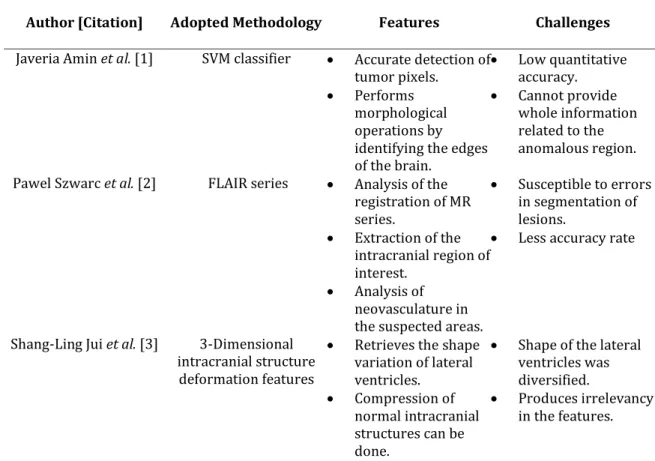
The literature has come out with several techniques for the detection and classification of brain tumor (Table I). However, they require more enhancements because of the low performance in the classification process. The SVM classifier used in [1] provides accurate detection of tumor pixels by performing morphological operations for the identification of edges in the brain. But it cannot provide complete information regarding the anomalous
region in the brain. Moreover, the FLAIR series used in [2] can be used for the analysis of registration of MR series and the neovasculature by extracting the intracranial region of interest. But it was susceptible to errors in the segmentation of lesions. Furthermore, 3-D intracranial structure deformation features employed in [3] can be used to get the shape variation of the lateral ventricles and thus compression can be done in the normal intracranial structures for the detection of tumor. But it produces irrelevancy in the features of the images. The two-tier classifier used in [4] can be used to classify the brain tumor depending on the double training process and thus eliminates the noise from the image; still, it includes several complexities in selecting the features from the image. The Local Binary Patterns and Histogram Orientation Gradient used in [5] can be used for the identification and separation of ROI from the background of the image, but there occurs degradation in the performance during the detection of tumor. FCM and ensemble based SVM classifier used in [6] can be employed for the extraction of texture features from the noise-free images for the detection and classification of tumors. But it cannot deal with some of the issues that occurred in the image. ANFIS used in [7] can be used to differentiate the abnormal tumor cells from the healthy brain cells, but it was susceptible to inter-expert variability. CEEMDAN and Hilbert transformation used in [8] can be used to calculate the quantitative metrics for the classification of tumor cells, but the performance obtained during the classification process is very low.
Table 1: Features and challenges of brain tumor detection and classification techniques Author [Citation] Adopted Methodology Features Challenges Javeria Amin et al. [1] SVM classifier Accurate detection of
tumor pixels.
Performs morphological operations by identifying the edges of the brain. Low quantitative accuracy. Cannot provide whole information related to the anomalous region. Pawel Szwarc et al. [2] FLAIR series Analysis of the
registration of MR series. Extraction of the intracranial region of interest. Analysis of neovasculature in the suspected areas.
Susceptible to errors in segmentation of lesions.
Less accuracy rate
Shang-Ling Jui et al. [3] 3-Dimensional intracranial structure
deformation features
Retrieves the shape variation of lateral ventricles. Compression of normal intracranial structures can be done.
Shape of the lateral ventricles was diversified.
Produces irrelevancy in the features.
V. Anitha and S.
Murugavalli [4] Two tier classifier Classifies the brain tumor in double training process
Eliminates noise and stripes the skull from the image. High system performance. Complexity in selecting the features. Classification accuracy was low for the real images.
Solmaz Abbasi and
Farshad Tajeripour [5] Local Binary Patterns and Histogram Orientation
Gradient
Pre-processing of the image can be done.
Identification and separation of ROI from the background of the image.
Degradation in the performance of tumor detection
Less accuracy rate. Quratul Ain et al. [6] FCM and ensemble based
SVM classifier Extraction of texture features from the noise-free images.
Extraction and separation of tumor region from the normal brain cells.
Cannot deal with some of the issues in the images
Very low-intensity values.
P. Shantha Kumar and P.
Ganesh Kumar [7] ANFIS Differentiates the abnormal tumor cells from the healthy brain cells.
Seems to be an effective technique. Susceptible to inter-expert variability. Increasing computation need. Taranjit Kaur et al. [8] CEEMDAN and Hilbert
transformation Calculates the quantitative metrics for the classification of tumor cells.
Calculates the density measure from the formulated density vector.
Less proximity limit.
Decrease in classification performance.
III. WORKING STRATEGY OF PROPOSED BRAIN TUMOUR DETECTION
The architecture of proposed model is shown in Fig 1. The input will be the MRI brain image. Four major contributions of this work are (i) Preprocessing (ii) Segmentation (iii) Feature Extraction and (iv) Classification. In the pre-processing stage, there performs two process include contrast enhancement and skull stripping. Under the contrast enhancement, high contrast regions can be easily detected. Meanwhile, as doing the skull stripping, the non-brain tissues like skull, scalp, dura, eyes will be removed. The resultant pre-processed image is given for segmentation process using FCM, in which it segments the images into four clusters specifically white matter, grey matter, Cerebrospinal fluid (CSF) and the abnormal tumour regions. Then the segmented tumor image, is subjected to feature extraction process. Both the GLCM and GLRM are used to extract the texture features. Finally, the extracted features are given for optimized DBN classification, in which the optimization of features and number of hidden layers are done via GWO optimization algorithm. The classification results the output image in two criteria:
Preprocessing
This is the initial process, where the contrast enhancement and skull stripping process is performed.
Contrast enhancement: The contrast of resized input image I is improved in this step. The specific process adjusts the intensity of image [26] and therefore the visibility of image gets highly enhanced by adopting relative darkness and brightness of I, which is specified in Eq. (1), where denotes the contrast enhancement of image. Thus, the present I converts into new grey level image. The contrast-enhanced image is denoted as Ic.
low out out low out high gamma in low in high in low I CO IC _ _ _ * ^ _ _ / _ Skull stripping [27]: This is a vital pre-processing approach, which eradicates the skull part from the brain image. The working principle of skull-stripping is given below:
(1)Read the contrast-enhanced image, C I .
(2)Binarize the image and get the binarized image as C
bin
I , IbinC binarization(IC).
(3)Identify the highly related component c1 from
C bin I .
(4)Dilate c1 with 3˟3square structuring element 2
SE , cˆ1c1SE2.
(5)Fill the holes in the final image (resultant image) as in Eq. (2). Continue until 1 ˆ 1 ˆ 1 ˆ ˆ k k c c
C c k k c SE I cˆ1ˆ 1ˆ1 2 (2) (6) Image regions are segmented from the original image CI with respect to cˆ1kˆ, and obtain the skull stripped image as the preprocessed image Ip.
Segmentation
FCM [41] is an algorithm that is particularly utilized for image segmentation. In this paper, the resultant Ip is given as the input to FCM. The segmentation is achieved by separating the image spaces into numerous cluster regions with same image’s pixels values. The traditional FCM is as follows:
Step (1) Select the arbitrary centroid at least 2 and put random values.
Step (2) Evaluate the membership matrix as in Eq. (3), where m1 and cl is the cluster’s number.
cl k m k i j i ij cl x cl x ME 1 ˆ 1 2 ˆ | | 1 (3)Step (3) Evaluate the cluster center as in Eq. (4).
m i m ij m i i m ij ME x ME cc 1 1 (4) Step (4) If
k k ccccˆ1 ˆ then stop, otherwise go to step 2.
The segmented image S
I is subjected for extracting features.
Feature Extraction
For any image processing technique, feature extraction is considered a major process, and in this paper, GLCM features with GRLM features are extracted from S
I .
GLCM [29] is defined as a procedure that extracts the second order statistical texture features. The procedure models the relationship between pixels that present in region by constructing GLCM This algorithm is on the basis of inference of second order mutual limited functions (Probability Density Functions), pr
n,m|di,
for varied direction
135 , 90 , 45 , 0
, so on, and the unlike distance di=1, 2, 3, 4 and 5. The pr
n,m|di,
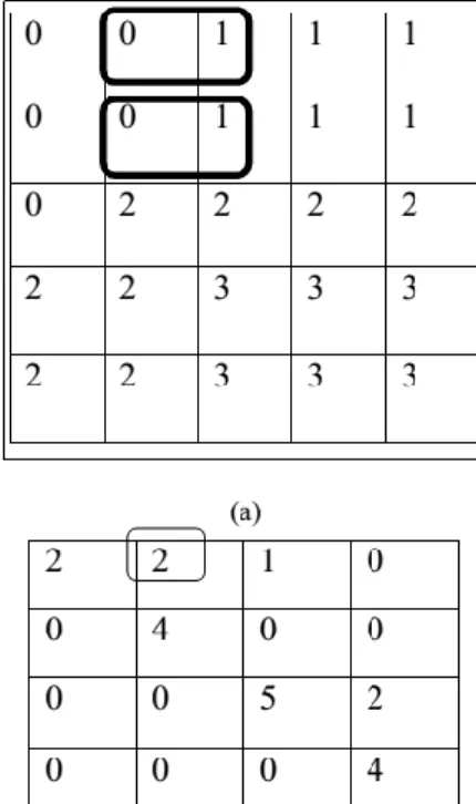
function is the probability with 2 pixels that are placed in an inter-sample distance di and direction, which also has the grey level n andm. Here, the spatial relationship is determined in correspondence with di and . If the present texture is coarse, and di is small, the pixels pair at di must has same gray values. Conversely, for the fine texture, the pixel couple at di must often is quite unlike, and hence the value in GLCM must be stretching out moderately and uniformly. In the same way, if the available texture is coarser in a single direction over another, then the degree of values spread about the major diagonal in GLCM must differ with Fig 2 illustrates the development of GLCM of grey-level, g (4 levels) image at di= 1 and = 0°.
Fig 2: (a) Image with 4 grey level 2 (b) GLCM for
di
=1 and =
0⁰
Fig 2(a), the box denotes the pixel-intensity 0 with pixel intensity 1 since its neighbour is in =0⁰. There exist two incidence of this pixel pair. So, the GLCM matrix
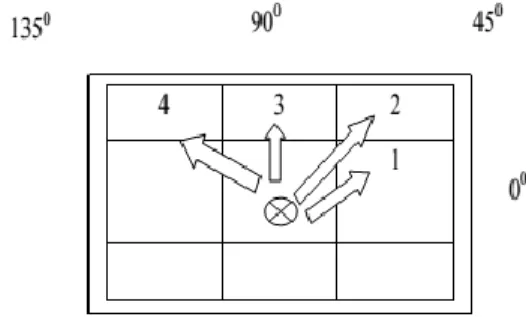
produced with value 2 in row 0 and column 1. This procedure is continued for additional intensity value pair. With this effect, the pixel matrix illustrated in Fig 2(a) could be changed into GLCM as given in Fig 2(b). Further to the direction (0⁰), GLCM could be formed for all other directions 45⁰, 90⁰, and 135⁰ as represented in Fig 3.
Fig 3: Directions 45⁰, 90⁰ and 135⁰
GLCM matrix is the assessment of the second order joint conditional probability, co of one gray level y to another gray level z with inter-sample distance di and the given direction by angle. The GLCM features are given in Table 2. Table 2: GLCM features Features Formulas Energy
z y z y co EN , 2 , Contrast
z y z y co z y CON , 2 , Entropy
z y z y co z y co ENT , 2 , log , Variance
yz y z g i VAR
2 ;is mean Homogenei ty
y z
gyz z y HOM 2 1 1 Correlation
j i y z j i yz g yz COR
Sum average
g N y j i y yg SA 2 2 Sum Entropy
g j i N y j i y g y g SE 2 2 log Sum Variance
g N y j i y g SA y SV 2 2 2 Differencevariance Differencevariancevarienceof gij Difference
entropy DifferenceEntropy g
y
gi j
y
N y j i g
log 1 0GRLM: GRLM [29] is a matrix, which gives the texture features for the analysis of texture. This is the process of searching image, always on given direction, for runs of pixels having the similar value of gray level. The Run length is the count of neighboring pixels that
have the same grey intensity in a specific direction. GRLM matrix is a 2-dimensional matrix, in which each element is the count of elements jwith iintensity, in direction. Hence, given a direction, the run-length matrix measures for each acceptable gray level value how many times there are runs of. GRLM matrix is as given in Eq. (5), whereUgdenotes the utmost grey level, max
L denotes the maximum length. In GRLM, a run-length matrixMR
i,j and grey level lengthMg
i,j is determined as the number of runs with pixel of bothi grey level and jrun length in numerous directions for image. NRdenotes the number of runs and Npdenotes the number of pixels. The GRLM features are in Table III.
g
i,j |
,0iUg,0 jLmax (5) Table 3: GRLM featuresFeatures Formulas
Short Run Emphasis
N j R R j j M N SRE 1 2 1 ;Long Run Emphasis
N j R R j j M N LRE 1 2 1Grey level
non-uniformity
K i g R i M N GLN 1 2 1 Run percentage p R N N RP Low grey level runemphasis
K i g R i i M N LGRE 1 2 1High grey level run
emphasis
K i g R i i M N MGRE 1 2 1Short run Low grey
level emphasis
K i N j R i j j i M N SRLGE 1 1 2 2 , 1Short run High grey
level emphasis
K i N j R j i j i M N SRHGE 1 1 2 2 , 1Long run Low grey
level emphasis
K i N j R i j j i M N LRLGE 1 1 2 2 , 1Long run High grey
level emphasis
K i N j R j i j i M N LRHGE 1 1 2 2 , 1 ClassificationThe featuresFare given as the input to DBN
classifier. DBN [36] model is a renowned intelligent approach established in 1986. Normally, it comprises of multiple layers, and each layer has visible neurons that establish the input layer, and hidden neurons form the output layer. Additionally, there has a deep connection with hidden and input neurons; however there was no connection between hidden neurons and no connections are available in the visible neurons. The connection between visible and hidden neurons is symmetric as well as exclusive. This respective neuron model determines an accurate output for the input. As the stochastic
neurons’ output in Boltzmann network is probabilistic, Eq. (6) specifies the output and Eq. (7) gives the possibility in sigmoid-shaped function, where tP
specifies the pseudo-temperature. The deterministic approach of stochastic model is given in Eq. (8).
P t q e O 1 1 (6)
q q O with O with PR 0 1 1 (7)
0 1 0 2 1 0 0 1 1 lim lim 0 0 for for for e O P P P t t q t (8) The diagrammatic illustration of DBN model is in Fig. 4, where the feature extraction process takes place by a set of RBM layers and the classification process takes place using Multi-Layer Perceptron (MLP). The mathematical approach exposes the energy of Boltzmann machine for the formation of neuron or binary statebi, which is given in Eq. (9), where wa,l specifies the weights between neurons and adenotes the biases.
al a l a a bi w bi E
, (9)The descriptions of energy regarding the joint composition of visible and hidden neurons
x,y are given in Eq. (10), Eq. (11) and Eq. (12). From the stated descriptions, xadenotes either the binary or neuron state of avisible unit, Wlrefers to the binary state of l hidden unit, and kaand Wadenotes the biases that applied in the network.
l a l a a a l a l a l a x y k x Wy w y x E
, , , (10)
l a l al a y w y k x E ,
(11)
a l l al a w x W y x E ,
(12) The possibility dissemination of input data is encoded into weight (parameters), and it is spread as the learning pattern of RBM. RBM training can achieve the dispersed possibilities, and the subsequent weight assignment is determined by Eq. (13). c
x w N x w M ˆ ˆ max ˆ (13) For all pair of visible and hidden vectors
x,hi , the possibility assigned RBM model is defined in Eq. (14), where FPA specifies the partition function as in Eq. (15).
E xy F e PA hi x c 1 , , (14)
y x y x E F e PA , , (15)Fig 4: Architecture of DBN model
This model uses Contrastive Divergence (CD) learning as the gaining of sampling expectations is a complex process under distribution. The CD algorithm steps are as follows:
Step 1: Select the xtraining samples and brace it into visible neurons.
Step 2: Assess the possibilities of hidden neuronscy by finding the product of wˆweight matrix and visible
vectorxascy
x.wˆ based on Eq. (16).
a l a a l l x W x w y c 1| , (16) Step 3: Observe they hidden states fromcy probabilities.Step 4: Assess the xexterior product of vectors and y
c , which are considered as positive gradient tP y c x. . Step 5: Inspect the reconstruction of xvisible states
from y hidden states as in Eq. (17). Furthermore, it is required to examine y hidden states from the reconstruction ofx.
a l a l a l y k xw x c 1| , (17) Step 6: Assess the exterior product of xandy, by itas negative gradient P t y x . .
Step 7: Determine the updated weight as in Eq. (18), where specifies the learning rate.
wˆ (18)
Step 8: Eq. (19) gives the weight update with new values. l a l a l a w w w, , , (19) Before beginning the learning process by MLP algorithm, consider
NM RM
ˆ ˆ
, training patterns, where
Mˆ specifies the number of training patterns,1Mˆ O,
M
N ˆ and RMˆ
vectors, respectively. Each neuron error in lof output
layer is shown in Eq. (20). M M M
l N R
eˆ ˆ ˆ (20) Thus, Eq. (20) gives the squared error ofMˆ pattern followed by MSE (Mean Squared Error) as in Eq. (21).
~
2 1 ˆ ˆ 2 ~ 1 ˆ ˆ ~ 1 ~ 1
y oy l M M y o l M l y mean M o e o N R SE (21) mean M avg SE O SE 1~ ˆ (22) The subsequent steps give the process of DBN training with RBM training (pre-training) and MLP training (normal).Step 1: DBN model is initialized with weights, biases and other related parameters that are randomly chosen.
Step 2: Initially, RBM model initialization processed with the input data, which serves the potentials in its visible neurons and conveys the unsupervised learning.
Step 3: The input to the consequent layer is conquered by sampling the potentials, which progressed in the hidden neurons of the previous layer. Furthermore, it follows the unsupervised learning.
Step 4: The aforementioned steps are continued for a particular number of layers. Thus the pre-training stage by RBM is done till it touches the MLP layer.
Step 5: MLP phase denotes the offered learning by supervised format, and it sustained till it achieves the target error rate.
The classifier outputs the respective detection of the existence of tumour in brain image with respect to high accuracy rate.
IV. PROPOSED OPTIMIZED DETECTION MODEL Solution Encoding and objective function
The solution encoding of the proposed GW-DBN model is given in Fig 5. This solution will be the input to GWO algorithm, which gives the optimal result for detecting brain tumour in image.
Fig 5: Architecture of DBN model
The objective function,O of proposed model is in Eq.
(23).
DBN Accuracy
Max
O (23)
Grey Wolf Optimization
This paper uses GWO to optimize the obtained featuresFalong the hidden neurons of DBN. GWO [30] is
a renowned meta-heuristic algorithm that mimics both the leadership and hunting mechanism of grey wolves. GWO includes four different levels: the first level is the alpha, thewolves are specified as the leaders of the troop (either male and female). They also have the power of taking decisions related to the hunting, walking time, sleeping place, and so on. The second level is
termed as beta that aidsin taking decisions. The third level is termed as delta , and it is called as subordinates. Finally, the last level is omega, and it is named as the scapegoat. In GWO algorithm all the three
, and guides in hunting procedure.
The mathematically model of encircling behavior is in Eq. (24).
tr X tr X B A| P (24)
tr
X
tr C A X 1 P (25)wheretrdenotes the present iteration, CandB
denotes the coefficient vectors, P X
refers to the position vector of prey, X
specifies the position vector of grey wolf. The assessment of CandBis defined in Eq.(26)
and Eq. (27), wheremiis linearly minimized from 2 to 0,
1
v andv2are the random vectors in the range [0,1].
mi v mi C2 1 (26) 2 2 v B (27)
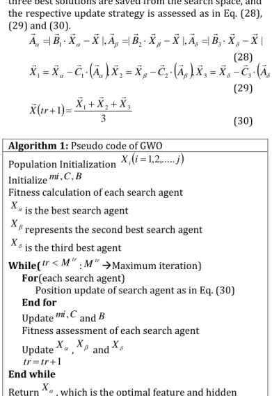
Generally, guides the hunting process. The leading three best solutions are saved from the search space, and the respective update strategy is assessed as in Eq. (28), (29) and (30). | | |, | |, |B1 X X A B2 X X A B3 X X A (28)
C A X X C A X X C A X X 1 2 2 3 3 1 , , (29)
3 1 X1 X2 X3 tr X (30) Algorithm 1: Pseudo code of GWOPopulation Initialization Xi
i1,2,...j
Initializemi,C,BFitness calculation of each search agent
X is the best search agent
X represents the second best search agent
X is the third best agent While(trMtr: tr
M Maximum iteration) For(each search agent)
Position update of search agent as in Eq. (30) End for
Updatemi,CandB
Fitness assessment of each search agent UpdateX,X andX 1 tr tr End while
ReturnX, which is the optimal feature and hidden
neuron
The final, and position might be the random position in the search space. Algorithm 1 shows the pseudo code of GWO. The final position will be the
optimal feature and hidden neuron that highly works for the optimal detection of brain tumor.
V. RESULTSANDDISCUSSIONS Experimental Setup
The proposed brain tumor detection using MR image was implemented in MATLAB 2014a. The used database
from URL
(https://www.ncbi.nlm.nih.gov/pmc/articles/PMC4833 122/ ) consists of both normal and abnormal images. Especially, the dataset presents 29 normal images and 29 abnormal images. The proposed algorithm compares its performance over conventional algorithms like NB [33], SVM [34], NN [35], DBN [36] and conventional optimization algorithms like GA [37], PSO [38], ABC [39] and FF [40], respectively by varying the learning percentage to 30, 50, 60, 70 and 80.
Performance Analysis
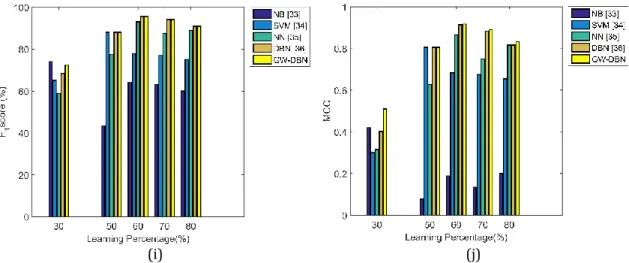
In this section, the performance of the proposed method is proven over the conventional classifiers like NB, SVM, NN and conventional DBN by varying the learning percentage to 30, 50, 60, 70 and 80. The analytical result is shown in Fig 5. Here, Fig 5. (a) gives the accuracy result of the proposed model over conventional methods. From the graph, it is proven that the proposed method has attained better performance in terms of accuracy (for all learning percentage). Especially, for learning percentage, 30%, the proposed GW-DBN is 9.41%, 16.24%, 16.90% and 16.41% better from the conventional methods like DBN, NN, SVM, and NB, respectively. For 60% learning, the proposed GW-DBN is 0.67%, 6.17%, 19.54% and 65.81% better than DBN, NN, SVM, and NB, respectively. For learning percentage, 70%, the accuracy of proposed method is 0.74%, 3.65%, 13.32% and 62.61% better than DBN, NN, SVM, and NB, respectively. The proposed method attains better sensitivity than the conventional methods, which is evident in Fig 5 (b). Fig 5 (b) shows that for 30% learning, the proposed method is 0.60%, 27.48%, and 0.49% better than conventional DBN, NN, SVM, and NB, respectively. For 50% learning, the proposed method is 0.11% better than DBN and 14.18% better than NN methods. For 60% learning, the proposed method gives the superior sensitivity rate, which is 2.46% superior to NN, 45.79% superior to SVM and 27.30% superior to NB methods. For 70% learning, the proposed method is 4.38%, 42.79%, and 43.85% better from NN, SVM, and NB, respectively.
Further, the proposed method attains higher specificity than the other methods. Especially for 30% learning, the proposed method is 7.78%, 4.26%, 30.79% and 63.82% better than the methods like DBN, NN, SVM, and NB, respectively. For 50% learning, the proposed method gives higher performance, which is 1.43%, 6.34%, 1.66% and 40.76% better than DBN, NN, SVM, and NB, respectively. For 60% learning, the proposed method is 38.75%, 6.15%, 0.94% and 50.96% better than DBN, NN, SVM, and NB, respectively. For learning percentage, 70%, the performance of proposed method is 11.01%, 11.56%, 0.39% and 61.36% better than DBN, NN, SVM, and NB, respectively. The precision of
proposed method is highly enhanced than the conventional methods, which is shown in Fig 5 (d). Here, for 30% learning, the performance of proposed method is 11.47%, 14.13%, 23.04% and 36.80% better than the conventional methods like DBN, NN, SVM, and NB, respectively. For 50% learning, the precision of proposed method is 0.17%, 9.96%, 0.79% and 82.10% superior to DBN, NN, SVM, and NB, respectively. For 60% learning, the proposed method is 10.35%, 5.502%, 0.60% and 71.89% better than DBN, NN, SVM, and NB, respectively. For 70% learning, the proposed method is 10.55%, 13.64%, 0.97% and 84.78% better from DBN, NN, SVM, and NB, respectively.
The FNR of proposed method is very low, and for 30% learning, the proposed method is 98.57%, 22.44%, and 3.02% better from DBN, NN and SVM, respectively. For 50% learning, the proposed method is 3.20%, 34.21%, 6.54%, and 67.79% better than DBN, NN, SVM, and NB, respectively. For 60% learning, the proposed method is 86.17%, 66.12%, and 54.14% superior to the methods like NN, SVM, and NB, respectively. For 70% learning, the proposed method is 15.53%, 70.29%, and 55.40% better from NN, SVM, and NB, respectively. The NPV of proposed method is highly improved than the conventional methods, which is illustrated in the graph Fig 5 (g). The NPV of proposed method for 30% learning is 22.33%, 10.28%, 39.73% and 65.84% better than DBN, NN, SVM, and NB, respectively. For 50% learning, the NPV of proposed method is 0.89%, 8.10%, 1.05% and 37.07% superior to DBN, NN, SVM, and NB, respectively. For 60% learning, the proposed method is 9.88%, 5.87%, 1.24% and 99.17% better than DBN, NN, SVM, and NB, respectively. For 70% learning, the NPV of proposed method is 11.48%, 12.17%, 0.68%, 60.97% better from the methods like DBN, NN, SVM, and NB, respectively. The FDR of proposed method is gradually minimized than the conventional methods, which is shown in Fig 5 (h). From the graph, it is evident that for 30% learning, the proposed method is 33.22%, 35.34%, 48.88%, and 56.93% superior to DBN, NN, SVM, and NB, respectively. For 50% learning, the proposed method is 4.87%, 92.06%, 16.12% and 98.19% better than DBN, NN, SVM, and NB, respectively. For 60% learning, the attained FDR of proposed method is 95.36%, 93.47%, 58.69% and 98.26% better from DBN, NN, SVM, and NB, respectively. For 70% learning, the FDR of proposed method is 96.24%, 96.85%, 45.12% and 99.07% better than DBN, NN, SVM, and NB, respectively.
Similarly, the performance of proposed method in terms of MCC is shown in Fig 5 (j). It is evident that for 30% learning, the proposed method is 35.89%, 70.96%, 76.66% and 26.19% better from DBN, NN, SVM, and NB, respectively. For 50% learning, the performance of proposed method in terms of MCC is 1.28%, 27.41%, 2.59%, 2.59% and 81.01% better from DBN, NN, SVM, and NB, respectively. For 60% learning, the MCC of proposed method is 2.17%, 8.04%, 44.61% and 80.85% better from DBN, NN, SVM, and NB, respectively. For 70% learning, the proposed method is 3.57%, 22.53%, 27.94% and 91.95% better than DBN, NN, SVM, and NB, respectively. Thus, the observation proves the
superiority of proposed method in terms of accurate diagnosing. (a) (b) (c) (d) (e) (f) (g) (h)
(i) (j)
Fig 6: Analytical result of proposed GW-DBN over conventional classifiers by varying the learning percentage (a) Accuracy (b) Sensitivity (c) Specificity (d) Precision (e) FPR (f) FNR (g) NPV (h) FDR (i)
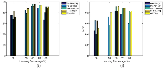
F1Score (j) MCC Effectiveness of GWO
Fig 6 illustrates the performance of GW-DBN algorithm over other conventional algorithms like GA-DBN, PS-GA-DBN, ABC-GA-DBN, and FF-DBN. Fig 6 (a) gives the accuracy performance of proposed approach. Here, for 50% learning, it is evident that the proposed method is 0.13%, 15.28%, 8.17% and 79.80% better than the conventional methods like FF-DBN, ABC-DBN, PS-DBN, GA-DBN, respectively. For 60% learning, the accuracy of proposed method is 7.99%, 0.32%, 8.12% and 94.13% superior to FF-DBN, ABC-DBN, PS-DBN, GA-DBN, respectively. For 70% learning, the accuracy of proposed method is 2.41%, 0.64%, 3.91% and 5.48% better from the methods like FF-DBN, ABC-DBN, PS-DBN, GA-DBN, respectively. The specificity of proposed approach as shown in Fig 6 (c) reviews that for 50% learning, the proposed method is 0.63%, 27.06%, 8.54% and 0.41% better than FF-DBN, ABC-DBN, PS-DBN, GA-DBN, respectively. For 60% learning, the developed GW-DBN is 22.01%, 9.07%, 21.62% and 0.83% superior to FF-DBN, ABC-FF-DBN, PS-FF-DBN, GA-FF-DBN, respectively. For 70% learning, the proposed GW-DBN is 0.86% better than FF-DBN, 1.07% better than ABC-FF-DBN, 35.63% better than PS-DBN and 37.97% better than GA-DBN.
Moreover, the proposed approach has attained less FDR, and the result is clearly demonstrated in Fig (e). For the learning percentage 30%, the proposed method is 38.76%, 46.99%, and 70.43% better than FF-DBN, ABC-DBN, GA-DBN, respectively. For 50%, the proposed method attains less FPR, which is 92.45%, 99.81%, 99.51% and 93.65% superior to FF-DBN, ABC-DBN, PS-DBN, GA-PS-DBN, respectively. For 60% learning, the developed method is 97.76%, 96.24%, 97.75% and 47.43% better from the methods like FF-DBN, ABC-DBN, PS-DBN, GA-DBN, respectively. FDR result of both
proposed and conventional approaches are shown in Fig 6. (h). The graph shows that for 30% learning, the proposed method attains better results, which is 3.92%, 35.51%, and 42.97% better than FF-DBN, ABC-DBN, GA-DBN, respectively. For 50% learning, the proposed approach is 64.81%, 99.15%, 97.98% and 45.71% superior to the approaches like FF-DBN, ABC-DBN, PS-DBN, GA-PS-DBN, respectively. For 60% learning, the proposed approach is 96.47%, 93.88%, 96.23% and 41.93% better from the conventional FF-DBN, ABC-DBN, PS-DBN, GA-DBN, respectively. The F1Score performance of proposed model is illustrated in Fig 6 (i). For 50% percentage, the proposed approach is 0.72% better than FF-DBN, 12.67% better from ABC-DBN and 5.61% superior to PS-DBN. For 60% learning, the proposed GW-DBN is 4.85% superior to FF-DBN, 3.43% better than ABC-DBN and 5.24% better from PS-DBN. For 70% learning, the proposed method is 2.64%, 1.26%, 4.84% and 5.73% better from FF-DBN, ABC-DBN, PS-DBN, GA-PS-DBN, respectively. The MCC of proposed approach is given in Fig 6 (j). From the given graph, it is clear that the proposed method for 50% learning is 1.23%, 43.85%, and 13.85% better than FF-DBN, ABC-DBN, PS-ABC-DBN, respectively. For 60% learning, the proposed approach is 9.52%, 3.37% and 10.84% superior to FF-DBN, ABC-DBN, PS-DBN, respectively. For 70% learning, the proposed method has attained high MCC, which is 1.12%, 16.88%, and 18.42% better from FF-DBN, PS-DBN, GA-DBN, respectively. Hence, the above analysis proves the performance of proposed method over other conventional approaches in terms of the optimal result.
(a) (b)
(c) (d)
(e) (f)
(i) (j)
Fig. 7. Performance of GWO over conventional algorithms by varying the learning percentage (a) Accuracy (b) Sensitivity (c) Specificity (d) Precision (e) FPR (f) FNR (g) NPV (h) FDR (i) F1Score (j) MCC Performance Analysis
This section explains the overall performance of proposed GW-DBN over other methods, which is in Table 4. It is reviewed that the accuracy of GW-DBN is 0.39%, 67.32%, 15.83% and 7.56% better from conventional DBN, NB, SVM, and NN, respectively. The sensitivity of proposed model is 18.51%, 42.22% and 1.58% superior to NB, SVM, and NN, respectively. FNR of GW-DBN is 55.55% and 70.37% better than NB and SVM models. F1Score of proposed model is 49.01%, 22.35%, and 7.56% better from NB, SVM and NN, respectively. The MCC of proposed model is 0.79%, 84.83%, 31.84% and 18.51% superior to conventional DBN, NB, SVM, and NN, respectively. Hence the analysis has proven the improved performance of proposed model over other methods in diagnosing the presence of brain tumor.
Table 4. Overall Performance of Proposed brain tumor detection Model
Measures NN [33] SVM [34] NB [35] DBN [36] GW-DBN Accuracy 0.875 0.8125 0.5625 0.9375 0.94118 Sensitivity 0.875 0.625 0.75 1 0.88889 Specificity 0.875 1 0.375 0.875 1 Precision 0.875 1 0.54545 0.88889 1 FPR 0.125 0 0.625 0.125 0 FNR 0.125 0.375 0.25 0 0.11111 NPV 0.875 1 0.375 0.875 1 FDR 0.125 0 0.45455 0.11111 0 F1-score 0.875 0.76923 0.63158 0.94118 0.94118 MCC 0.75 0.6742 0.13484 0.88192 0.88889
Table 5 tabulates the overall performance of GWO over other optimization methods. The accuracy of GWO is 0.39% and 3.52% better from FF and ABC models, and 7.56% superior to PSO and GA models. The sensitivity of GWO is 1.58% and 6.66% better than FF and ABC models, respectively. The F1Score of GWO is 0.84% and 3.52% superior to both FF and ABC models, 5.88% better than both PSO and GA models. The MCC of GWO is 0.79% and 6.66% better from FF and ABC models, 14.75% better from both PSO and GA models. Hence, the total analysis has proven the betterments of GWO in precise detection of disease.
Table 5. Overall Performance of GWO over conventional meta heuristic algorithms
Measures GA [37] PSO [38] ABC [39] FF [40] GWO
Accuracy 0.875 0.875 0.90909 0.9375 0.94118 Sensitivity 1 1 0.83333 0.875 0.88889 Specificity 0.75 0.75 1 1 1 Precision 0.8 0.8 1 1 1 FPR 0.25 0.25 0 0 0 FNR 0 0 0.16667 0.125 0.11111 NPV 0.75 0.75 1 1 1 FDR 0.2 0.2 0 0 0 F1_score 0.88889 0.88889 0.90909 0.93333 0.94118 MCC 0.7746 0.7746 0.83333 0.88192 0.88889 VI. CONCLUSIONS
A new way of brain tumor detection model has been introduced in this paper. The model has included several stages like Preprocessing, Segmentation, Feature Extraction and Classification processes. Two fundamental processes like contrast enhancement and skull stripping were processed under initial phase, and FCM segmentation was performed in Segmentation phase. Both GLCM and GRLM features were extracted in the phase of feature extraction. Moreover, this paper has used DBN for classification. The DBN was integrated with GWO optimization approach to get the optimal result in the detection of brain tumor. The proposed GW-DBN model has compared its performance over other methods in terms of Accuracy, Specificity, Sensitivity, Precision, NPV, F1Score MCC, FPR, FNR, and FDR. The results obtained tells that the accuracy of GW-DBN was 0.39%, 67.32%, 15.83% and 7.56% better from conventional DBN, NB, SVM and NN, respectively. The sensitivity of proposed model was 18.51%, 42.22% and 1.58% superior to NB, SVM, and NN, respectively. FNR of GW-DBN was 55.55% and 70.37% better than NB and SVM models. F1Score of proposed model was 49.01%, 22.35%, and 7.56% better from NB, SVM and NN, respectively. Thus, the performance of proposed model for detecting brain tumor was proven over other methods.
REFERENCES
[1] Javeria Amin, Muhammad Sharif, Mussarat Yasmin and Steven Lawrence Fernandes, "A Distinctive Approach to Brain Tumor Detection and Classification using MRI," Pattern Recognition Letters, vol. 10, pp. 116- 156, October 2017.
[2] Pawel Szwarc, Jacek Kawa, Marcin Rudzki and Ewa Pietka, "Automatic brain tumour detection and neovasculature assessment with multiseries MRI analysis," Computerized Medical Imaging and Graphics, vol. 46, pp. 178-190, December 2015. [3] S. L. Jui et al., "Brain MRI Tumor Segmentation with 3D
Intracranial Structure Deformation Features," in IEEE Intelligent Systems, vol. 31, no. 2, pp. 66-76, Mar.-Apr. 2016.
[4] V. Anitha and S. Murugavalli, "Brain tumour classification using two-tier classifier with adaptive segmentation technique," in IET Computer Vision, vol. 10, no. 1, pp. 9-17, 2 2016.
[5] Solmaz Abbasi and Farshad Tajeripour, "Detection of brain tumor in 3D MRI images using local binary patterns and histogram orientation gradient," Neurocomputing, vol. 219, pp. 526-535, January 2017.
[6] Quratul Ain, M. Arfan Jaffar and Tae-Sun Choi, "Fuzzy anisotropic diffusion based segmentation and texture basedensemble classification of brain tumor," Applied soft computing, vol. 21, pp. 330-340, August 2014.
[7] P. Shanthakumar and P. Ganeshkumar, "Performance analysis of classifier for brain tumor detection and diagnosis," Computers and electrical engineering, vol.45, pp. 302-311, July 2015. [8] T. Kaur, B. S. Saini and S. Gupta, "Quantitative metric for MR brain
tumour grade classification using sample space density measure of analytic intrinsic mode function representation," in IET Image Processing, vol. 11, no. 8, pp. 620-632, 8 2017.
[9] Xiaomei Zhao , Yihong Wu , Guidong Song , Zhenye Li ,Yazhuo Zhang and Yong Fan, "A deep learning model integrating FCNNs and CRFs for brain tumor segmentation," Medical image analysis, vol. 43, pp. 98-111, January 2018.
[10]T. Ramakrishnan and B. Sankaragomathi, "A Professional Estimate on the Computed Tomography Brain Tumor Images using SVM-SMO for ClassiÞcation and MRG-GWO for Segmentation," Pattern recognition letters, vol. 94, pp. 163-171, July 2017.
[11]B. Gholami, I. Norton, L. S. Eberlin and N. Y. R. Agar, "A Statistical Modeling Approach for Tumor-Type Identification in Surgical Neuropathology Using Tissue Mass Spectrometry Imaging," in IEEE Journal of Biomedical and Health Informatics, vol. 17, no. 3, pp. 734-744, May 2013.
[12]Elisee Ilunga Mbuyamba, Juan Gabriel Avina Cervantes, Jonathan Cepeda Negrete, Mario Alberto Ibarra Manzano and Claire Chalopin, "Automatic selection of localized region-based active contour models using image content analysis applied to brain tumor segmentation," computers in biology and medicine, vol. 91, pp. 69-79, December 2017.
[13]M. Huang, W. Yang, Y. Wu, J. Jiang, W. Chen and Q. Feng, "Brain Tumor Segmentation Based on Local Independent Projection-Based Classification," in IEEE Transactions on Biomedical Engineering, vol. 61, no. 10, pp. 2633-2645, Oct. 2014.
[14]Yan Zhu and Zhu Yan, "Computerized tumor boundary detection using a Hopfield neural network," in IEEE Transactions on Medical Imaging, vol. 16, no. 1, pp. 55-67, Feb. 1997.
[15]J. J. Corso, E. Sharon, S. Dube, S. El-Saden, U. Sinha and A. Yuille, "Efficient Multilevel Brain Tumor Segmentation With Integrated Bayesian Model Classification," in IEEE Transactions on Medical Imaging, vol. 27, no. 5, pp. 629-640, May 2008.
[16]A. Islam, S. M. S. Reza and K. M. Iftekharuddin, "Multifractal Texture Estimation for Detection and Segmentation of Brain Tumors," in IEEE Transactions on Biomedical Engineering, vol. 60, no. 11, pp. 3204-3215, Nov. 2013.
[17]A. Demirhan, M. Törü and İ. Güler, "Segmentation of Tumor and Edema Along With Healthy Tissues of Brain Using Wavelets and Neural Networks," in IEEE Journal of Biomedical and Health Informatics, vol. 19, no. 4, pp. 1451-1458, July 2015.
[18]A. Hamamci, N. Kucuk, K. Karaman, K. Engin and G. Unal, "Tumor-Cut: Segmentation of Brain Tumors on Contrast Enhanced MR Images for Radiosurgery Applications," in IEEE Transactions on Medical Imaging, vol. 31, no. 3, pp. 790-804, March 2012. [19]A. P. Nanthagopal and R. Sukanesh, "Wavelet statistical texture
features-based segmentation and classification of brain computed
tomography images," in IET Image Processing, vol. 7, no. 1, pp. 25-32, February 2013.
[20]Neha Rani and Sharda Vashisth, "Brain Tumor Detection and Classification with Feed Forward Back-Prop Neural Network," International journal of computer applications, vol. 146, no. 12, July 2016.
[21]G Rajesh Chandra and Kolasani Ramchand H Rao, "Tumor Detection In Brain Using Genetic Algorithm," computer science, vol. 79, pp. 449-457, 2016.
[22]D. M. Joshi, N. K. Rana and V. M. Misra, "Classification of Brain Cancer using Artificial Neural Network," 2010 2nd International Conference on Electronic Computer Technology, Kuala Lumpur, pp. 112-116, 2010.
[23]K.Sudharani, T.C.Sarma Dr. and K. Satya Prasad Dr., "Advanced Morphological Technique for Automatic Brain Tumor Detection and Evaluation of Statistical Parameters," Technology, vol. 24, pp. 1374-1387, 2016.
[24]Vasupradha Vijay, Dr.A.R.Kavitha and S.Roselene Rebecca, " Automated Brain Tumor Segmentation and Detection in MRI using Enhanced Darwinian Particle Swarm Optimization(EDPSO)," Computer science, vol. 92, pp. 475-480, 2016.
[25]Khan M. Iftekharuddin, Jing Zheng, Mohammad A. Islam and Robert J. Ogg, "Fractal-based brain tumor detection in multimodal MRI," Applied mathematics and computation, vol. 2017, pp. 23-41, 2009.
[26]Iza Sazanita Isa, Siti Noraini Sulaiman, Muzaimi Mustapha and Noor Khairiah A. Karim, "Automatic contrast enhancement of brain MR images using Average Intensity Replacement based on Adaptive Histogram Equalization (AIR-AHE)," Biocybernetics and Biomedical Engineering, vol. 37, no. 1, pp. 24-34, 2017.
[27]S. Roy and P. Maji, "A simple skull stripping algorithm for brain MRI," 2015 Eighth International Conference on Advances in Pattern Recognition (ICAPR), Kolkata, pp. 1-6, 2015.
[28]M. Shasidhar, V. S. Raja and B. V. Kumar, "MRI Brain Image Segmentation Using Modified Fuzzy C-Means Clustering Algorithm," 2011 International Conference on Communication Systems and Network Technologies, Katra, Jammu, pp. 473-478, 2011.
[29]A.Harshavardhan, Suresh Babu and T. Venugopal, "Analysis of Feature Extraction Methods for the Classification of Brain Tumor Detection," International Journal of Pure and Applied Mathematics, vol. 117, no. 7, pp. 147-155, 2017.
[30]SeyedaliMirjalili, Seyed MohammadMirjalili and AndrewLewis, "Grey Wolf Optimizer", Advances in Engineering Software, vol.69, pp.46-61, March 2014.
[31]R. Kaur and S. Kaur, "Comparison of contrast enhancement techniques for medical image," 2016 Conference on Emerging Devices and Smart Systems (ICEDSS), Namakkal, pp. 155-159,2016.
[32]A. Alsam, I. Farup and H. J. Rivertz, "Iterative sharpening for image contrast enhancement," Colour and Visual Computing Symposium (CVCS), pp. 1-4 Gjovik, 2015.
[33]V. Muralidharan and V. Sugumaran, " A comparative study of Naïve Bayes classifier and Bayes net classifier for fault diagnosis of monoblock centrifugal pump using wavelet analysis", Applied Soft Computing, vol. 12, pp. 2023–2029, 2012.
[34]David Meyera, FriedrichLeisch and Kurt Hornik, " The support vector machine under test", Neurocomputing, vol. 55, pp. 169 – 186, 2003.
[35]Yogeswaran Mohan, Sia Seng Chee, Donica Kan Pei Xin and Lee Poh Foong, " Artificial Neural Network for Classification of Depressive and Normal in EEG", 2016 IEEE EMBS Conference on Biomedical Engineering and Sciences (IECBES), 2016.
[36]H.Z. Wang, G.B. Wang⇑, G.Q. Li, J.C. Peng, and Y.T. Liu, " Deep belief network based deterministic and probabilistic wind speed forecasting approach", Applied Energy, vol. 182, pp. 80–93, 2016. [37]John McCall, " Genetic algorithms for modelling and optimisation",
Journal of Computational and Applied Mathematics, vol. 184, pp. 205–222, 2005.
[38]M.E.H. Pedersen and A.J. Chipperfield, " Simplifying Particle Swarm Optimization", Applied Soft Computing, vol. 10, pp. 618– 628, 2010.
[39]D. Karaboga and B. Basturk, " On the performance of artificial bee colony (ABC) algorithm", Applied Soft Computing, vol. 8, pp. 687– 697, 2008.
[40]A.H. Gandomia, X.-S. Yang, S. Talatahari, and A.H. Alavi, "Firefly algorithm with chaos", Commun Nonlinear Sci Numer Simulat, vol. 18, pp. 89–98, 2013.
[41][41] Hind Rustum Mohammed, Husein Hadi Alnoamani and Ali AbdulZahraa, " Improved Fuzzy C-Mean Algorithm for Image Segmentation", (IJARAI) International Journal of Advanced Research in Artificial Intelligence, vol. 5, no. 6, 2016

