This is an Open Access document downloaded from ORCA, Cardiff University's institutional repository: http://orca.cf.ac.uk/114553/
This is the author’s version of a work that was submitted to / accepted for publication. Citation for final published version:
Yu, Han, Chapman, Brian, Di Florio, Arianna, Eischen, Ellen, Gotz, David, Jacob, Mathews and Blair, Rachael Hageman 2019. Bootstrapping estimates of stability for clusters, observations and model selection. Computational Statistics 34 (1) , pp. 349-372. 10.1007/s00180-018-0830-y file Publishers page: http://dx.doi.org/10.1007/s00180-018-0830-y
<http://dx.doi.org/10.1007/s00180-018-0830-y> Please note:
Changes made as a result of publishing processes such as copy-editing, formatting and page numbers may not be reflected in this version. For the definitive version of this publication, please refer to the published source. You are advised to consult the publisher’s version if you wish to cite
this paper.
This version is being made available in accordance with publisher policies. See
http://orca.cf.ac.uk/policies.html for usage policies. Copyright and moral rights for publications made available in ORCA are retained by the copyright holders.
Bootstrapping estimates of stability for clusters,
observations and model selection
Han Yu, Brian Chapman, Arianna DiFlorio, Ellen Eischen, David Gotz, Mathews Jacob and Rachael Hageman Blair
Han Yu
State University of New York at Bu_alo Department of Biostatistics 3435 Main Street 706 Kimball Tower Bu_alo, NY 14214 hyu9@bu_alo.edu Brian Chapman University of Utah
Department of Radiology and Imaging Science 729 Arapeen Drive
Salt Lake City, UT 84108 Tel.: 801-587-8672
Arianna DiFlorio
Institute of Psychological Medicine and Clinical Neurosciences (current) Cardi_ University School of Medicine
Hadyn Ellis Building Maindy Road Cathays
Cardi_ CF24 4HQ
diorioa@cardi_.ac.uk
University of North Carolina at Chapel Hill (previous) Department of Psychiatry
University of North Carolina at Chapel Hill Campus Box 7160 Chapel Hill, NC 27599 [email protected] Ellen Eischen University of Oregon Department of Mathematics 315 Fenton Hall Eugene, OR 97403-1222 Tel.: (541) 346-5633 [email protected]
David Gotz
University of North Carolina at Chapel Hill School of Information and Library Science University of North Carolina at Chapel Hill 216 Lenoir Drive, Campus Box 3360 Chapel Hill, NC 27599
Tel.: 919-962-3435
Mathews Jacob University of Iowa
Department of Electrical and Computer Engineering
3314 Seamans Center for the Engineering Arts and Sciences Iowa City, Iowa 52242
Tel.: (319) 335-6420
Corresponding Author: Rachael Hageman Blair
State University of New York at Bu_alo Department of Biostatistics 3435 Main Street 709 Kimball Tower Bu_alo, NY 14214 Tel.: 726-829-2814 hageman@bu_alo.edu
Bootstrapping estimates of stability for clusters,
observations and model selection
Han Yu, Brian Chapman, Arianna DiFlorio, Ellen Eischen, David Gotz, Mathews Jacob, Rachael Hageman Blair*
Abstract Clustering is a challenging problem in unsupervised learning. In lieu of a gold standard, stability has become a valuable surrogate to performance and robustness. In this work, we propose a non-parametric bootstrapping approach to estimating the stability of a clustering method, which also captures stability of the individual clusters and observations. This flexible framework enables different types of comparisons between clusterings and can be used in connection with two if possible bootstrap approaches for stability. The first approach, scheme 1, can be used to assess confidence (stability) around clustering from the original dataset based on bootstrap replications. A second approach, scheme 2, searches over the bootstrap clusterings for an optimally stable partitioning of the data. The two schemes accommodate different model assumptions that can be motivated by an investigator's trust (or lack thereof) in the original data and additional computational considerations. We propose a hierarchical visualization extrapolated from the stability profiles that give insights into the separation of groups, and projected visualizations for the inspection of the stability of individual operations.
Our approaches show good performance in simulation and on real data. These approaches can be implemented using the R package bootcluster that is available on the Comprehensive R Archive Network (CRAN).
Keywords ensemble - k-means - Jaccard coeffcient - clustering – visualization
This work was supported by the National Science Foundation. HY and RHB were both sup- ported through NSF DMS 1557589, and RHB also through NSF DMS 1312250. BC was sup- ported through NSF DMS 1557576. EE was supported through NSF DMS 1557642. MJ was supported through NSF DMS 1557668. AD and DG was supported through NSF DMS 1557593.
*Corresponding Author
State University of New York at Bu_alo Department of Biostatistics 3435 Main Street 709 Kimball Tower Bu_alo, NY 14214 Tel.: 726-829-2814 E-mail: hageman@bu_alo.edu
1 Introduction
Clustering is used to group items in a dataset based on similarity. Generally, the clustering problem can be framed as an optimization problem, where the objective is to maximize the similarity within a group, and minimize the similarity between groups (Jain et al., 1999). However, performance and robustness is difficult to quantify and are very much a function of the data set at hand. In lieu of a gold standard, the stability of a particular clustering of a dataset can be used as a surrogate for performance and robustness.
Various definitions, applications and estimations of stability have emerged in recent years. The overarching aim of stability is to capture how stable the clusterings are over several different representations of the data (Von Luxburg, 2009). These data representations are derived either through subsetting, cross-validation, data noising or re-sampling, among others. Different data representations have the potential to reveal different characterizations of stability for a clustering. Recently, Von Luxburg (2009) provided a survey on the use of stability for clustering data that emphasizes the sensitivity of the underlying structure to these data representations. Stability based on subsampling is an intuitive example of where this sensitivity can be readily observed, especially when the subsets are small. Another intuitive example is when the stability estimate is generated by adding noise to the data, which can easily erode any signal of structure, and give rise to misleading results (Hennig, 2007). Briey, we provide a basic overview of approaches to stability estimation for clustering, but refer the reader to Von Luxburg (2009) for a more comprehensive survey.
The bootstrap (Efron and Tibshirani, 1994) has been leveraged to connect ensemble clustering and cluster stability estimation. Felsenstein (1985) used a non-parametric bootstrap (Efron et al., 1996) to infer phylogenetic trees in one of the earliest examples of re-sampling for various summarizations over an ensemble of dendrograms. Kerr and Churchill (2001) proposed a residual bootstrap that shuffles residuals from an analysis of variance (ANOVA) model of gene expression data. Clusters from the bootstrap data were compared to the original clusterings to assess confidence in the various clusters. This approach is model-based in the sense that the ANOVA model _t is required to obtain residuals, and also requires a suitable experimental design. Dudoit and Fridlyand (2003) propose applications of bagging to clustering that frames the unsupervised problem as the supervised classification problem of predicting cluster labels. Two bootstrapping schemes were proposed, BagClust1 determines cluster membership by consensus from a bootstrap and permutation scheme, and BagClust2 derives a new dissimilarity matrix based on bootstrapped data that is then used for input for another round of clustering (Dudoit and Fridlyand, 2003). In both approaches, improvements in accuracy were observed.
Fang and Wang (2012) proposed the use of the non-parametric bootstrap for the estimation of the number of clusters, k. The estimation of stability that they propose is a function of pairwise comparisons between B bootstrap samples. For each pair of bootstrap samples, the original data is projected onto the bootstrap clusterings, and distance between the projections is calculated using binary indicators, see Fang and Wang (2012) for details. The mapping of the data to the bootstrap clusterings is not explicitly described. For k-means, a possibility is to assign membership based on the distance to the closest center, but in hierarchical clustering, this may require the use of a pre- defined linkage. Improvements were
observed over a cross-validation approach proposed by Wang (2010), which overestimates the instability of the clustering due to bias arising from the fold assignments.
Clustering over various subsets of the data is another approach to stability estimation. Ben-Hur et al. (2001) characterize stability through pairwise similarities of clusterings obtained from random subsets of the observations. Similarity is based on the Jaccard distance between cluster labels for the random subsets. High similarities between observations suggests a stable clustering, and the authors demonstrate that this approach is a reliable way to select the number of clusters, and to assess the overall lack of structure in the data (Ben-Hur et al., 2001).
Tibshirani and Walther (2005) proposed a method for estimating the number of clusters by re-casting the unsupervised problem into a supervised classification problem, similar in spirit to Dudoit and Fridlyand (2003). Framing the problem in this way enables the calculation of prediction strength, which quantifies how well a clustering with k groups can be predicted by the data. Prediction strength is used for the purpose of model selection. For each k, repeated cross-validation is used to form training and test datasets, and prediction strength is calculated pairwise for observations in the test data. Specifically, the training and test data is clustered separately for a fixed k. The test data is then projected onto the training clustering. For example, in the k-means setting, this projection amounts to membership labels based on the nearest centroid. For all pairs assigned to the same cluster in the test data, those pairs that are also assigned the same cluster (or not) in this projection are deemed to have a stable co-membership (or not). For each cluster, the proportion of co-members that stably map together when projected onto the training set is then computed, and the prediction strength is defined to be the minimum of these proportions.
Within the prediction strength framework, an estimate of prediction strength at the individual observation level is also defined (Tibshirani and Walther, 2005). Similar to calculations at the cluster level, the estimation of prediction strength at the individual observation level is done in a pairwise manner. The estimate of prediction strength for an individual, i, is estimated as the proportion of pairs (i; i0) in the test cluster Ak(i) that map to together with i when projected onto the training set, is the proportion of pairwise co-memberships for all i0 6= i, within the assigned cluster in the test data that stably map together when projected onto the training set. In this work, we also emphasize stability at the individual level, but define it as an estimate of how stable an individual maps to the same cluster across bootstrap samples. Hennig (2007) proposed a method to estimate cluster-wise stability through bootstrapping and other re-sampling approaches. In this framework, the stability of an original cluster is estimated by the mean maximal Jaccard coefficient. The stability measure is specific to the clustering of the original data, as the comparisons are made between all of the re-sampled clusterings, and the original data clustering. A limitation of this approach is the implicit requirement of mapping between the re-sampled and original clusters. Importantly, during the re-samplings, it is possible that an original cluster is not detected through the mapping. When this occurs, the method simply ignores the re-sampled clusterings for the estimation for that cluster. Consequently, this can potentially lead to an overestimation of stability, since a cluster that does not consistently emerge during re-samplings is actually an indication of instability that is not accounted for. In addition, as a measure of cluster similarity, the maximal
Jaccard coefficient is not symmetric (although the Jaccard coefficient itself is symmetric). Due to asymmetricity, a one-to-one mapping between clusters arising from different clusterings is not guaranteed, thus searching for maximum will tend to result in an overestimation. In this work we propose stability estimates based on the non-parametric boot-strap. Our approaches offer several advantages over existing methods for stability estimation. (1) To our knowledge, this is the first bootstrapping approach for cluster stability that can guide in the determination of the number of clusters and also retains valuable interpretations of stability at the level of the cluster and individual observation. (2) Two bootstrapping approaches to stability are developed that reflect different model assumptions, which can be motivated by an investigator's trust (or lack thereof) in the original data. Specifically, the first approach, scheme 1, can be used to assess confidence (stability) around clustering from the original dataset based on bootstrap replications. Whereas, a second approach, scheme 2, searches over the bootstrap clusterings for an optimally stable partitioning of the data. (3) Both bootstrap approaches directly estimate the conditional stability through comparisons between clusterings that depend on symmetric measure of cluster similarities. (4) Different visualizations are proposed, such as hierarchical visualizations extrapolated from stability profiles that reflect separation and stability of inferred clusters and projected visualizations for the inspection of individual stability. In this work, we focus on k-means, but the approach can be generalized to other clustering methods. The R (https://www.r-project.org/) package, bootcluster, is available on the Comprehensive R Archive Network (CRAN) and supports bootstrap stability estimation using these approaches.
2 Methods
In this section, we outline different approaches to estimating cluster stability that are based on non-parametric bootstrapping. The objective is to estimate how stable the clustering is (1) overall, (2) at the cluster level, and (3) at the individual observation level. This is achieved through the estimation of cluster centers for the original data and bootstrapped datasets, the projection of the data onto the partitions estimated from the bootstrapped datasets, and the comparisons of these mappings. Two bootstrapping schemes are illustrated in Figure 1, which differ in the nature of their comparisons. Scheme 1 (Figure 1A) depicts a scenario in which the clusterings arising from the bootstrapped datasets are directly compared to the clustering of the original data. In scheme 2 (Figure 1B), the clusterings arising from the bootstrapped datasets are compared to the clusterings of the original data, and to each other. These approaches can be implemented using the R package bootcluster that is available on CRAN. In the following sections, we propose two approaches that can be used to make the comparisons that underly the stability estimates used in scheme 1 & 2 (Figure 1).We define naive stability (Section 2.1) as estimates that rely on the crude indicators (0-1) to capture a stable mapping, or lack thereof, when the data points are _t to the bootstrapped centers. An alternative approach is presented that utilizes the Jaccard index (Section 2.2) to estimate the stability in the same basic framework. For simplicity, we develop these approaches for the k-means algorithm, but the methods are generalizable to other prototype and non-prototype methods. More-over, we describe the naive and Jaccard-based formulations within the scheme 1 framework, but these formulations are used in connection with both bootstrapping schemes, and are both implemented in our applications.
2.1 Bootstrapping estimation of naive stability
In this work, we define naive stability in a straightforward manner. By applying a clustering algorithm to a dataset, each observation included is assigned a cluster label. If we have a bootstrapped sample, then new cluster assignments will be obtained, which leads to a different partition of the feature space. This causes changes in the labels of some observations and also in the members of certain clusters. The observations that switch labels frequently across bootstrap re-samplings are regarded as unstable. Therefore, the naive stability of an observation can be measured by the frequency that it remains in a cluster across re-samplings.
This procedure is outlined in Algorithm 1, where X = (X1;X2; : : : ;Xn)T is the sample of size n, and Xb is the data set from bth re-sampling. The notation C is used to denote a clustering, with Cb as the clustering on the bth re-sampled data. Further, Cb i denotes the set of data points in the ith cluster of Cb, while C(Xi) is the set of all data points in the cluster that contains Xi. A limitation to the naive approach is that clusters from different re-samplings have to be mapped to each other. In our applications, the minimum Euclidean distance between cluster centers is used for the mapping. Note that in Algorithm 1 and 2, the number of clusters, k, is fixed for the calculation of bootstrapped stability. In practice, this algorithm should be implemented several times over a range of k values to estimate the number of clusters. 2.2 Bootstrapping estimation of Jaccard index based stability
For the naive estimation of stability proposed in Algorithm 1, we defined stability at the observation level as the probability of an observation consistently being as- signed to the same cluster. However, the naive stability estimation of Algorithm 1 requires the mapping between centers from different re-samplings. This can be an issue when a cluster is broken down into multiple smaller clusters in a re-sampled clustering. This problem can be circumvented by using the change in pairwise co-membership.
To motivate the use of the Jaccard coffcient, let us first consider the Hamming distance between clusterings, which are based on such pair-wise relationships. Let C and D be two clustering partitions of X, which is distributed as P. We use the notation xi _C xj , when xi and
xj belong to the same cluster of C, and xi _C xj otherwise. The Hamming clustering distance between two clusterings, C and D, is de_ned as:
where is the logical XOR operation. Along the same lines, the similarity between two clusterings can be de_ned as:
which is constructed based on agreements on each co-membership between two clusterings, C and D. Let the similarity at the individual level as:
Thus, the overall similarity can be decomposed in terms of each observation:
where, Sim(xi; C;D), can be expressed as:
Upon inspection of Sim (xi; C;D), it is immediately clear that the summation j6=i I(xi _C xj)I(xi _D xj) is expected
to be large and dominating, which will tend to send Sim(xi; C;D) ! 1. Ignoring this part, Sim(xi; C;D) can be redefined as:
The definition of overall similarity remains, except that the observation-wise similarity Sim(xi; C;D) is replaced by A(xi; C;D) in Equation(1):
Let C0; : : : ; CB be the clusterings obtained from original data and B re-sampled data sets, then we define conditional observation-wise and overall stability estimated as:
and unconditional overall stability:
Notably, unconditional cluster-wise stability cannot be defined. Moreover, although the unconditional overall stability can be defined, we emphasize that it is generally not useful because it does not reflect the feature of a specific clustering. Therefore, all the stability estimates in this study are conditional on a reference clustering. By this definition, we propose the Jaccard index based stability, and the bootstrapping approach for estimation in Algorithm 2. This algorithm proceeds similarly to Algorithm 1, but with some key differences. For each bootstrapped dataset, k-means is applied to obtain estimates of the centers mb. Note that each observation, xi, is then mapped to the closest center using Euclidean distance. Finally, the Jaccard coefficient is computed between the bootstrapped and reference clusterings. In these approaches, the fact that the bootstrapped datasets may contain repeated observations, and may omit some observations, is not problematic. This is because the bootstrapped dataset is used to update the mean estimates (centroids) in each iteration of k-means. If multiple instances occur in a data set, then within k-means, these multiple instances will be assigned the same cluster membership and used to update the means accordingly. On the other hand, if an observation does not occur, it will not enter into the clustering of the bootstrapped sample. However, once the k-means clustering has been carried out until convergence on the bootstrapped data, the means from the clustering are used to map each observation in the dataset, xi, to a cluster (xi ! mb) in order to obtain its membership, Cb(x), which is based on the minimum distance to the mean centers. This process can be understood in the first couple of lines within the for loops in Algorithm 1
2.3 Properties of Jaccard-based observation-wise stability estimation
We propose that A(xi; C;D) is a valid measure of observation-wise clustering similarity. Specific information is quantified from A(xi; C;D) about xi, and its value ranges from 0 to 1. When C(xi) and D(xi) have exactly the same members, we have A(xi; C;D) = 1, meaning clusterings C and D are identical with respect to xi, although C and D can be very different with respect to other observations. When C(xi) and D(xi) have completely different members except for xi, then A(xi; C;D) = 1 jC(xi)[D(xi)j ! 0 as jC(xi) [ D(xi)j ! 1. On the other hand, this is not true for Sim(xi; C;D). For example, if we have n = 100, and jC(xi)j = jD(xi)j = 10, then in the above case we will have A(xi; C;D) = 1=20 = 0:05, which is close to 0, while Sim(xi; C;D) = (1 + 80)=100 = 0:81. Inherently, Sim(xi; C;D) is very sensitive to both sample and cluster sizes, and the interpretation of simiPlarity and stability would vary among different data sets. Dropping the term j6=i I(xi _C xj)I(xi _D xj) would have the effect of scaling the support of A(xi; C;D) to approximately to (0; 1], and thus maintain consistent interpretation of the similarity and stability across data sets.
The measure, A(xi; C;D) = A(xi;D; C), is a symmetric measure of similarity between C and D with respect to xi. This property justifies the comparison of a fixed clustering with all other clusterings at the observation level, by which the conditional stability is defined. We propose that the conditional stability is important in that it retains the specific information for the reference clustering. We illustrate this concept with a simple example. Let C1; C2; : : : C101 be a set of 101 clusterings, based on the original data clustering and re-sampled clusterings. Suppose that C1(xi) \ Cj(xi) = fxig; j = 2; 3; : : : ; 101, and C2(xi) = _ _ _ = C101(xi). In addition, we assume jCj(xi)j = 10; j = 1; 2; :::; 101. The observation-wise clustering similarity is calculated as, A(xi; C1; Cj) _ 0:05; j = 2; : : : 101, and A(xi; Cj ; Ck) = 1, for 2 _ j 6= k _ 101. Furthermore, it can be shown that the conditional stability estimate (Equation 4) is Sobs(xi; C1) _ 0:05, while Sobs(xi; Cj) _ 0:99. The interpretation is that, the clustering of xi in C1 is unstable, but are stable in Cj ; j = 2; 3; : : : ; 101. However, if the unconditional overall stability (Equation 5) is used, then the estimates will be erroneously concluded that the results are generally stable, regardless of the clustering it refers to.
2.4 Bootstrapped estimate description in mathematical terms
The stability estimates arising from bootstrap schemes 1 and 2 (Figure 1) can be expressed as conditional and unconditional expectations, respectively. Let Xi be a random variable such that Xi _ F(x) and X = (X1;X2; : : : ;Xn)T , while Y is another independent sample drawn from the same distribution. Let CX denote the partition of sample space that corresponds to a sample X, and CX(x) denote the set of all points in sample space that are within the same partition of x. Then, wedefine the similarity between two partitions CX and CY with respect to x as:
and the overall similarity as: A(CX; CY) = Ex(A(CX; CY j x)):
The overall stability with respect to a sample X, which is estimated by scheme 1 (Figure 1A), can be defined as:
Sover(CX) = EXY(A(CX; CY) j CX);
where EXY takes the expectation over both X and Y. On the other hand, the unconditioned stability estimated by scheme 2 (Figure 1B) can be expressed as:
Sover = EXY(A(CX; CY)):
The individual stability is more meaningful in the conditioned scheme 2, and can be de_ned as:
Sobs (x j CX) = E (A(CX; CY j x) j CX) :
The cluster-wise stability is defined as the integration of Sobs(x j CX) within a corresponding partition with respect to x.
2.5 Estimation of k
The stability estimates can be used for selecting the number of clusters, k. For this purpose, the bootstrapping schemes should be carried out over a range of k values, resulting in a stability profile. However, instead of directly using the overall stability, we calculate cluster-wise mean Jaccard index during each re-sampling, record the minimum, and then average the minima across the B re-samplings. This measure is defined based on observation-wise similarity, such that it will have a large drop when ^k is greater than the true number of clusters k, and be independent of the value k. The overall stability does not always have such desirable properties. For example, when ^k = k+1, there will always be at least one group randomly split into at least two clusters, leading to a drop in stability. However, when k is large, this drop may be washed out in the average of stability, which is calculated over a large number of clusters. In contrast, the proposed measure, denoted by Smin, only records the minimal cluster-wise similarity from each re-sampling, such that the effects of random
splitting of groups will stand out, regardless of k. A similar minimum estimate is also utilized in the prediction strength method (Tibshirani and Walther, 2005).
2.6 Simulations
A series of simulations are used to assess and benchmark the performance of the proposed bootstrapping stability methods. Our first simulation sets out to examine the consequences from subsetting the data for stability estimation compared to the re-sampling bootstrap approach. We examined scheme 1 using a naive for mutation given in Algorithm 1 to compare estimates arising from subsets of the data of dwindling sizes. The naïve formulation given in Algorithm 1 allows for the direct comparison of the clustering results between the re-sampling and subsetting approach. For visual purposes, two clusters were simulated in two dimensions, the clusters are standard normal variables with (50; 50) observations per group, centered at (0; 0) and (2; 0), respectively.
Following Tibshirani and Walther (2005), we also simulated six scenarios to examine the performance with respect to selection of the number of clusters, k. The proposed bootstrap schemes were tested, along with the pairwise bootstrap pro- posed by Fang and Wang (2012) and prediction strength (Tibshirani and Walther, 2005). The pairwise bootstrap and prediction strength were implemented in the R programming language (https://www.r-project.org) using the package fpc. Each of the following simulations was performed 50 times.
1. Null model: A null model simulation was performed using 200 data points uniformly distributed over the unit square in ten dimensions.
2. Three-cluster model: Three clusters were simulated in two dimensions: the clusters are standard normal variables with (25; 25; 50) observations per group, centered at (0; 0), (0; 5) and (5;3).
3. Random four clusters in three dimensions: Four clusters were randomly chosen to have 25 or 50 multivariate normal observations with the covariance matrix as the identity matrix, I, and cluster centers randomly chosen from N(0; 5 _ I). Simulations with clusters having minimum distance less than 1:0 units between them were discarded.
4. Random four clusters in ten dimensions: Four clusters were randomly chosen to have 25 or 50 multivariate normal observations with the covariance matrix as the identity matrix, I, and cluster centers randomly chosen from N(0; 1:9 _ I). Simulations with clusters having minimum distance less than 1:0 units between them were discarded. In this and the previous scenario, the settings are such that about one-half of the random realizations were discarded.
5. Two elongated clusters: Two elongated clusters were simulated in three dimensions. Each cluster is generated as follows: set x1 = x2 = x3 = t with taking on 100 equally spaced values from 0:5 to 0:5 with Gaussian noise with standard deviation 0:1 is then added to each feature. A second cluster is generated in the same way, except that the value 10 is then added to each feature. The result is two elongated clusters, stretching out along the main diagonal of a three-dimensional cube.
6. Two close elongated clusters: Two close and elongated clusters were simulated in three dimensions. As in simulation five, a second cluster was generated in the same way as the first cluster. The value of 1:0 is then added to the first feature only.
The bootstrap approaches were applied to four different datasets that range in terms of complexity. Each dataset can be found in the UCI machine learning repository (Lichman, 2013). The iris and wine data are well-studied for classification and clustering. The iris data has 150 observations and four features. The wine data has 178 observations and 13 features. Iris and wine each have three classes that are not used for the clustering, but rather in a post hoc manner to assess performance.
The NCI60 microarray data set contains 64 samples representing 12 different types of cancer and 6; 830 gene expression features (Ross et al., 2000). The first two principal components (PCs) were used for clustering. The image segmentation data set was derived by randomly sampling from a database of 7 outdoor images (Lichman, 2013). The images were hand-segmented to create a classification for every pixel. The total of 2; 100 instances (observations) consist of 7 classes, with 300 observations per class. Although 19 features were present, six features were excluded due to redundancy or being uninformative. As with the iris and wine data sets, the class labels are not used in the clustering. To our knowledge, the image segmentation data has not been studied for clustering, whereas the other datasets have been. Linear discriminant analysis was applied to the image data in order to obtain a general assessment of the separability of the different classes of images (Hastie et al., 2001). For the real data examples, we constructed a hierarchical visualization of the clusters derived from the stability profile. The hierarchy is derived by first selecting the largest k with stability Smin above 0:9. These k's correspond to well-separated clusters, or the ones that can be easily detected by the algorithm. The second largest k with the stability Smin above 0:8 but below 0:9 is selected to represent finer cluster structures that are more challenging to detect (for example, more overlapped clusters).
3 Results
Stability estimation via repetitive subsetting is performed by randomly drawing a subset of observations without replacement multiple times (Ben-Hur et al., 2001; Tibshirani and Walther, 2005). Our first simulation was motivated by the fact that stability for prototype methods is closely related to the variability of centroids, which in turn is a function of sample sizes. Subsetting leads to a smaller sample size, and subsequently to an underestimation of stability and larger variance in estimates. Due to differences in defining clustering distances, stability or other characterizations of a clustering, estimates from different approaches are not directly comparable. For example, prediction strength (Tibshirani and Walther, 2005) and Boot2012 (Fang and Wang, 2012) rely on agreements of co-memberships, while Ben-Hur et al. (2001) uses Jaccard distance. However, all of them depend on the changes in item memberships. We examined the consistency of the predicted membership of a grid of data points in sample space between bootstrap resampling and repetitive subsetting in a balanced 2-cluster model (Figure 2). In this simple model, the exact mapping between resampled clusters and original ones is known, which enables the determination of membership switch. Figure 2A-C depicts the frequency of a point retaining its original membership on a gray scale. The light gray areas have low frequencies of membership changes, while those in darker gray areas tend to change membership more often. The differences between bootstrap resampling (Figure 2A) and repetitive subsetting with 1=2 the data (Figure 2B) are subtle, but the dark gray area (unstable region) for repetitive subsetting with 1=2 the data is larger than
that of the bootstrapping. Naturally, the effect is much more striking when repetitive subsetting with 1=4 of the data (Figure 2C). The bias and standard errors were also found to be higher for the repetitive subsetting (Figure 2D-E).
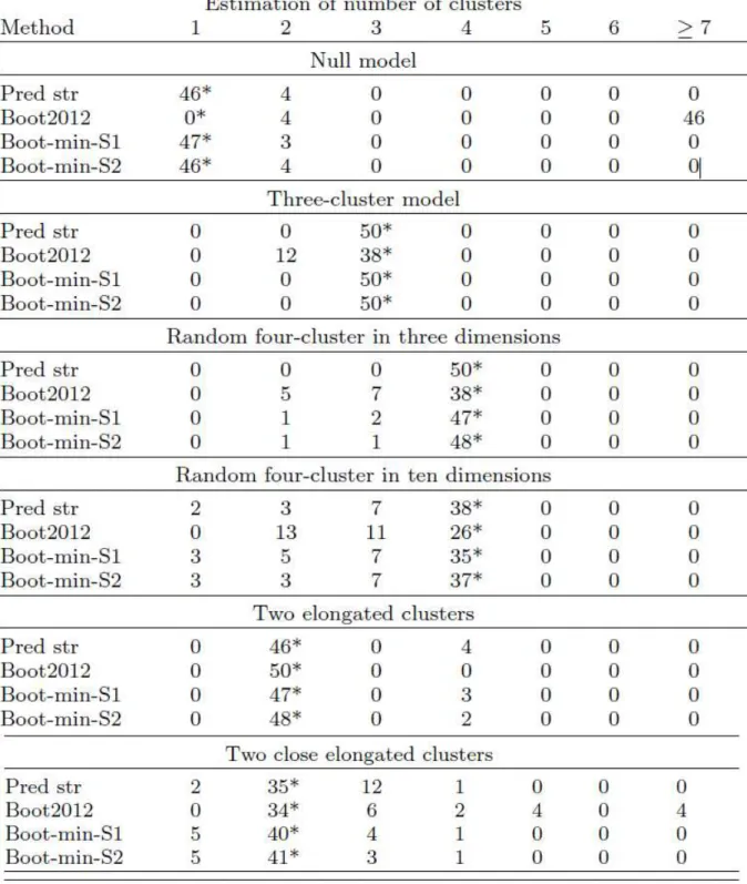
Bootstrapping stability based on the Jaccard index for the determination of the number of clusters, k, was also examined. Table 1 shows the performance of three methods for the selection of k for six classic simulation scenarios that were simulated 50 times and estimated using the prediction strength approach (Pred str) (Tibshirani and Walther, 2005), the pairwise bootstrap data comparisons method (Boot2012) (Fang and Wang, 2012), and our proposed Jaccard-based bootstrap estimate of stability using scheme 1 (Boot-min-S1) and scheme 2 (Boot-min-S2). Results indicate that our method is comparable, and in some scenarios outperforms prediction strength, while generally better than Boot2012. The stability profiles for difference settings are shown in Figure 3. The simulation results also support our argument that Boot2012 usually has poor performance for asymmetric settings
(three-cluster model and random four-cluster model) due to its criteria of maximum stability. Furthermore, this criteria also makes it impossible for Boot2012 to detect a null model. The difference between Boot-min-S1 and Boot-min-S2 is often subtle (Table 1), with Boot-min-S2 identical or slightly superior in all settings except for the null model estimation. With the exception of Boot2012, the errors in the selection of k are rather conservative in the sense that they tend to underestimate k, rather than overestimate. The proposed bootstrapping schemes clearly outperform both Boot2012 and Pred Str for the two close elongated cluster simulations (Table 1).
min-S1 and min-S2 were applied to the iris data, which has three classes. Boot-min-S2 suggests the correct number of clusters (k = 3) (Figure 4A), whereas Boot-min-S1 selects k = 2, with only a marginal difference in stability from Boot-min-S2. Comparatively, both prediction strength and Boot2012 imply two clusters due to the severe overlapping between species Virginica and Versi color in feature space (data not shown). This further illustrates the advantage of our method in dealing with asymmetrically distributed and overlapping clusters.
The individual stability plot includes three categories of stability, high (> 0:9), moderate (0:8
0:9) and low (< 0:8) (Figure 4C). The stability of the observa- tions for Boot-min-S2 (k = 3) naturally reveals more unstable points towards the boundaries of the clusters. For the iris data, we also considered two different representations of the data, one based on the first two PCs, and another using only sepal width and length. Visualizations of individual stability suggest that the less stable clusters (Supplemental Figure 1E) contain a higher proportion of unstable points (Supplemental Figure 1 C-D), as expected, which is a trend we will see in the other datasets.
With a pairwise distance, the clustering results can be projected into a clustering space using multi-dimensional scaling (MDS), where each clustering is represented as a point, and the clustering space can be visualized to observe the regions of high (black) and low (white) density (Figure 4E). Note that Equation (3) provides a Jaccard index based similarity that is a symmetric measure for each pair of the clusterings, A(Ci; Cj ), where 0 _ i; j _ B. Therefore, the distance between the clusterings can be de_ned as 1 A(Ci; Cj ).
The three classes in the wine data are approximately Gaussian distributed. Pred str, Boot2012, Boot-min-S1, and Boot-min-S2, all correctly indicate three clusters. Figure 4B shows the profile across different values of k for Boot-min-S1 and Boot-min-S2, respectively. The individual observation stability is viewed on PC axes (Figure 4D), although the clustering was done using all 13 features. The instabilities are naturally occurring at the boundaries, as these observations are more likely to change labels during repetitive re-sampling from the population. On the contrary, points in well separated clusters generally have higher stability levels. Figure 4F shows the re-sampled clusters using MDS. The clusterings selected by scheme 2 generally locate at the center of the points. Analogous to the minimization of average Euclidean distances by sample mean, scheme 2 can be viewed as an approach to obtaining an average of the bootstrapped clusterings, or a version of bagging.
The first two PCs of the NCI data were used to cluster the cancer samples. Application of the Boot-min-S2 method revealed three clusters (Figure 5A-B). Prediction strength (Tibshirani and Walther, 2005) indicated no cluster structure (1 cluster), which may be due in part to the smaller sample size and heterogeneity of the tumor samples. The effect of subsetting on exaggerating the variability of cluster centers is more severe for a small data set. Boot2012 (Fang and Wang, 2012) suggests _ 20 clusters. Figure 5C-E indicate that all melanoma samples cluster together (Cluster 3) with high stability, while the samples at the boundary of Cluster 2 and 3 are less stable. The cluster assignments tend to keep samples from the same cancer together, with the exception of breast which is almost evenly spread over the three clusters (Figure 5E). Examination of individual bootstrap samples (Supplemental Figure 3) reveals known challenges for the k-means algorithm due to the disparity in cluster shape, specifically elongation and imbalance between groups. Notably, the NCI microarray data does not show any clear cluster structure if the genes are used instead of a PCs. In this case, both prediction strength and Boot-min-S2 again indicate k = 1, and Boot2012 suggests k _ 20.
The image segmentation dataset consists of overlapping features and a larger number of classes (seven). The stability analysis suggests four clusters by a criteria of 0:9 (Figure 6A). This threshold is very stringent, and is more suitable for better separated cases, as was seen in the simulation settings. If we relax it to 0:8 to allow larger extent of overlap, then six clusters will be detected (Figure 6A). Figure 6B shows the clustering result in a PC space. It has been reported that the k-means clustering may not be optimal for image dataset, because even when the true number of classes is used (k = 7), the agreement between cluster and class labels is still low (Falasconi et al., 2010). This is also apparent in our clustering result (Figure 6E) Individual observation stability (Figure 6C) and cluster stability (Figure 6D) indicates that clusters 5 and 6 have highest stability, which corresponds to a
large proportion of sky and grass samples (Figure 6E). Visualizing these points, it becomes more apparent that the stability of a cluster depends on the proportion of unstable points and the degree of their instability. The least stable cluster (cluster 1 in Figure 6B) is comprised of nearly all points in a moderate stability range, it is thus clear that the stability of this cluster would be in the moderate range (_ 0:81). Clusters 2-4 also have lower stabilities, and pairs (Clusters 1 and 3, and Clusters 2 and 4), are more similar (Figure 6E). This may be due to the fact that these classes are less separable. To further investigate this, we performed linear discriminant analysis and found that cement, foliage and window are poorly classified when compared to sky and grass (Supplemental Table 1).
4 Discussion
The stability of a clustering captures the uncertainty of groupings and has been widely used to characterize the results, primarily in the context of model selection. Stability has been defined in a variety of ways that derive from different data representations such as bootstrapping, subsetting, or cross-validation. In this work, we have proposed two schemes for estimating stability via non-parametric bootstrap. A major advantage of both schemes is that stability can be estimated overall, as well as at the cluster and individual observation levels, which offers deeper insights into cluster structure and enables higher flexibility in model selection (e.g., Smin estimation). Moreover, because of the symmetric measure of observation-wise clustering similarity, it becomes possible to condition all levels of stability on a reference clustering. Therefore, all stability-related results are with respect to the reference.
The difference between the two schemes for stability estimation is the clusterings that are compared. In scheme 1, the original data clustering is trusted in the sense that the stability is conditional on the inferred clusters from the original data. This scheme mimics classical applications of the bootstrap that aim to assess confidence of an estimate (Efron et al., 1996). However, in practice this may be not be ideal for noisy data. In scheme 2, the clustering of the original data is not trusted to the same degree. On the contrary, the data is bootstrapped to find the most representative clusters, which is determined through the pairwise comparisons of bootstrapped clusterings. Additional factors may play into deciding between scheme 1 and 2. From the point of view of stability estimates, scheme 2 will always produce more stable clusters, as it selects the most optimal from the exhaustive set of pairwise companions between clusterings. However, this requires massive computation. For model selection, scheme 2 will also always capture the overall stability calculated with scheme 1 by design. However, we hypothesize that there will be additional bias' in the stability estimates at the cluster and individual level using scheme 2. An area of future research will assess the utility of these approaches with out of bag estimates of stability to capture the generalization and predictive capabilities of clustering method to assign group membership to new samples (Breiman, 1996).
Within the bootstrapping schemes, the comparison between clustering can be made via naive or Jaccard-based estimates of stability. These have relatively similar formulations. However, the ways in which they compare clustering capture different features of the stability. The naive approach uses 0-1 indicators to record whether an observation changes cluster membership, and it relies on the mapping between clusters from different clustering results. In the case of k-means, this can be achieved through the minimal Euclidean distance between centroids. An important limitation of the naive approach is with respect to mapping and the inaccuracies that can arise when the clusters are nested, e.g., a cluster is broken into two smaller clusters in the bootstrapped clustering of the data. This issue arises because the similarity between clusterings is asymmetric for naive stability estimates. These can be avoided by tracking the changes in co-memberships be- tween different clusterings, as in Ben-Hur et al. (2001); Tibshirani and Walther (2005), among others. Our implementation of Jaccard-based stability is motivated by the idea of monitoring changes of co-memberships, and reflects our confidence in a clustering at various levels of the method, clusters, and individual samples.
A limitation of our approaches is the need to set a threshold for estimating k. In practice, a threshold of 0:9 works well when the clusters are well separated or mildly overlapped (Supplemental Figure 4). In our real data applications, when the boundaries are less clear, it is advantageous to take a more liberal threshold of 0:8. However, stability ranges and profiles may vary due to different characteristics of the data. In application, we strongly suggest a coupling of the stability profiles with a visualization of the hierarchical organization via a dendrogram, which may provide insights into the separations (or lack thereof) of a complex feature space. Taken together with the stability estimates of the individual clusters and samples, additional insight can be gained for the selection of k. Note that prediction strength (Tibshirani and Walther, 2005), also requires a similar form of thresholding for model selection. In fact, the same thresholds, 0:9 and 0:8, are used in their
examples.
In terms of comparisons, our methods are closest to the bootstrapping approach described in Fang and Wang (2012). The performance differences between our method and Boot2012 is due in part to the underlying definitions of stability and the distinct criteria for determining k. Boot2012 does not require thresholding, but suffers from other drawbacks. In our approach, we define stability at the observation level, which provides higher flexibility on the criteria. In particular, it enables estimation of Smin and the usage of a criteria similar to the prediction strength approach (Tibshirani and Walther, 2005). On the other hand, the usage of maximum stability as criteria for estimating k in Boot2012 makes it impossible to detect null structure, as the stability will always be 1 when ^k = 1. Such criteria also tends to be conservative when the data structure is asymmetric (Von Luxburg, 2009). This can be overcome by using other criteria such as thresholding. However, as discussed in Section 2.5, the change in overall stability when ^k > k depends on sample size and the drop in overall stability can be washed out in averaging, which may pose challenges in model selection. The definition of Boot2012 stability by using an overall measure precludes its usage of a threshold criteria.
The prediction strength approach can provide an estimate for the individual observation (Tibshirani and Walther, 2005). However, due to repeated k-fold cross validation, these estimate may be inaccurate. For example, in the case of k-means, the feature space is partitioned according to the minimum distance of a point to cluster centers. Therefore, there are two factors affecting the individual stability: location of true cluster centers and variation of the estimates for the centers. The variation of an estimator is usually a function of sample sizes. However, by only sampling a part from the original sample, as is done repeatedly in prediction strength, the variation of the estimates for centers are expected to be over-estimated, and result in an under-estimation in stability. This is not an issue for prediction strength when used for the selection of the number of clusters, k, because it takes the minimum (least stable cluster) as the conservative prediction strength estimate. However, at the individual level, this is not a possibility. We therefore believe that our approach offers less bias with respect to stability estimation of an individual observation, although investigation through a controlled simulation would be challenging. Notably, if we view the prediction strength as a surrogate for stability, then the measure on the similarity between two clusterings is asymmetric, which precludes the definition of conditional stability as in this study.
Hennig (2007) proposed an approach to estimate cluster-wise stability through using mean maximal Jaccard coffcient. However, the estimation can be inaccurate, because it implicitly requires mapping between re-sampled and original clusters, and as discussed, the maximal Jaccard coffcient as a cluster-wise similarity measure is asymmetric. Also, it does not provide any information of the stability of individual observation. On the other hand, our approach does not require this re-mapping and uses a symmetric measure of similarity. Moreover, the exibility of our approach enables the user to calculate stability with respect to the initial data clustering, as in Hennig (2007), but also enables a search over the bootstrap replicates for a more likely clustering (scheme 2).
In this work, we focus on k-means for simplicity. However, the methods described can be generalized to other clustering methods. In the case of k-means, observations are mapped to the prototypes (estimated means from bootstrappeddata b) xi ! mb estimated to obtain bootstrapped membership Cb(xi). Alternative methods can be used as long as the mappings are well-dined, e.g., linkage in hierarchical clustering. In fact, the bootstrap can be used as a means to bench-mark and select the best suited clustering methods for a particular data set via the overall stability estimates. An area of future research is to combine results across different clustering methods in an ensemble fashion. A hypothesis is that different methods capture different features of the population better than others, combinations across methods may improved cluster assignment if coupled or weighted by stability estimates.
In conclusion, the stability of a clustering offers insights into the quality of a method and clustering for a dataset. We have developed novel methods for stability estimates based on the non-parametric bootstrap. Our approaches perform well in the selection of the number of clusters, but also offer an additional layer of model interpretation at the cluster and individual level. The two proposed bootstrapping schemes provide stability estimates that react different forms of uncertainty in the data, which may reflect an investigator's lack of trust in the original data clustering and the data itself. Visual interpretations of stability have been proposed to complement the estimates and guide the investigator in assessing the results.
Tables
Table 1 Performance for identifying the number of clusters, k, for six different simulations of 50 datasets each. Results are shown for prediction strength (pred str), bootstrapping proposed by Fang et al. (Boot2012), and bootstrapping scheme 1 min-S1) and 2 (Boot-min-S2). The asterisk * indicates the true number of clusters.
Figure Legends
Figure 1: Schematics for bootstrapping schemes for estimating clustering stability. (A) Clusters are estimated from the data, C0. Bootstrap data sets are sampled from the data with replacement (B1; : : : ;Bp) and clustered (C1; : : : ;Cp). The bootstrap clusterings are compared only to the original clustering of the data, C_ 0, using a naive 0-1 approach to membership, or a Jaccard coefficient. (B) Similar to scheme A, clusters are estimated from the data and bootstrapped datasets. However, in addition to comparing the original data clustering to the bootstrapped clusterings, each of the bootstrapped clusterings is compared with each other, and the original data clustering.
Figure 2: Simulation of a simple balanced 2-cluster model that illustrates the bias and standard error captured by the naive bootstrapped stability and repeated subsetting stability approach. Heatmap depiction of frequencies of data points retaining their original memberships for (A) bootstrap resampling, (B) 1/2 sub-setting (middle), and (C) 1/4 subsetting (right). Blue is unstable and red is stable. The (D) bias and (E) standard errors of naive stability for bootstrap resampling and subsetting.
Figure 3: Stability profiles based on minimal cluster similarity from each resampling (Smin) for the different simulation experiments estimated via Jaccard based bootstrapping. For each simulated scenario, 50 simulations were performed across k = 1 : : : 7 using scheme 2. The vertical lines indicate the true cluster numbers and horizontal lines indicate a threshold criteria of 0:9 Simulation scenarios are for a (A) null model, (B) three-cluster model, (C) four clusters in three dimensions, (D) four clusters in ten dimensions, (E) two elongated clusters, and (F)two elongated close clusters.
Figure 4: Results for the iris and wine data. Stability profiles based on minimal cluster similarity from each re-sampling (Smin) for the two bootstrapping schemes for the (A) iris and (B) wine data. Individual stability for (C) iris and (D) wine are shown for stable (> 0:9), moderately stable (0:8 0:9) and unstable (< 0:8) points. Note that the stability is visualized on PC axis, although the clustering and stability estimation was performed using the entire datasets. MDS representation of the results for (E) iris and (F) wine data that is based on the symmetric distance measure for each pair of clusterings arising from bootstrapped samples. The density plots are constructed according to the Jaccard index-based distance between resampled cluster labels. The asterisk indicates the final clustering result from scheme 2, which resides near the center of the cloud, which may be interpreted as an average representation of the clusterings.
Figure 5: Results of the NCI dataset clustering. (A) Stability profile based on minimal cluster similarity from each re-sampling (Smin) for the NCI dataset. (B) Inferred cluster assignment from stability analysis. (C) Individual stability is shown for stable (> 0:9), moderately stable (0:8 0:9) and unstable (< 0:8) points. (D) Visual hierarchy depicts the three clusters that are well separated and their memberships. The cluster specific stability is indicated.
Figure 6: Results of the image dataset clustering. (A) Stability profile based on minimal cluster similarity from each re-sampling (Smin) for the image dataset. (B) Inferred cluster assignment from stability analysis. (C) Individual stability is shown for stable (> 0:9), moderately stable (0:80:9) and unstable (< 0:8) points.
(D) Stability of the inferred clusters. (E) Two-layer hierarchy constructed from the stability profile. The hierarchy reveals the data contains four well-separated clusters, while two among them can be further partitioned into two less separable ones (red dashed clades), respectively. The cluster specific stability is indicated.
References
Ben-Hur, A., Elisseeff, A., and Guyon, I. (2001). A stability based method for discovering structure in clustered data. In Paci_c Symposium on Biocomputing, volume 7, pages
6{17.
Breiman, L. (1996). Out-of-bag estimation. Technical report, Statistics Department, University of California Berkeley, Berkeley CA.
Dudoit, S. and Fridlyand, J. (2003). Bagging to improve the accuracy of a clustering procedure. Bioinformatics, 19(9), 1090{1099. Efron, B. and Tibshirani, R. J. (1994). An Introduction to the Bootstrap: Chapman & Hall/CRC Monographs on Statistics & Applied Probability. CRC Press, USA.
Efron, B., Halloran, E., and Holmes, S. (1996). Bootstrap con_dence levels for phylogenetic trees. Proceedings of the National Academy of Sciences, 93(23), 13429{13429.
Falasconi, M., Gutierrez, A., Pardo, M., Sberveglieri, G., and Marco, S. (2010). A stability based validity method for fuzzy clustering. Pattern Recognition, 43(4), 1292{1305.
Fang, Y. and Wang, J. (2012). Selection of the number of clusters via the bootstrap. Computational Statistics and Data Analysis, 56, 468{477.
Felsenstein, J. (1985). Con_dence limits on phylogenies: an approach using the bootstrap. Evolution, pages 783{791.
Hastie, T., Tibshirani, R., and Friedman, J. (2001). The Elements of Statistical Learning. Springer Series in Statistics. New York, NY, USA: Springer New York Inc.
Hennig, C. (2007). Cluster-wise assessment of cluster stability. Computational Statistics and Data Analysis, 52(1), 258{271.
Jain, A. K., Murty, M. N., and Flynn, P. J. (1999). Data clustering: a review. ACM Computing Surveys, 31(3), 264{323.
Kerr, M. K. and Churchill, G. A. (2001). Bootstrapping cluster analysis: assessing the reliability of conclusions from microarray experiments. Proceedings of the National Academy of
Sciences, 98(16), 8961{8965.
Lichman, M. (2013). UCI Machine Learning Repository. Ross, D. T., Scherf, U., Eisen, M. B., Perou, C. M., Rees, C., Spellman, P., Iyer, V., Jeffrey, S. S., Van de Rijn, M., Waltham, M., Permamenschikov, L., Lashkari, D., Shalon, D., Myers, T., Botstein, D., and Brown, P. (2000). Systematic variation in gene expression patterns in human cancer cell lines. Nature Genetics, 24(3), 227{235.
Tibshirani, R. and Walther, G. (2005). Cluster validation by prediction strength. Journal of Computational and Graphical Statistics, 14(3), 511{528.
Von Luxburg, U. (2009). Clustering stability: an overview. Foundations and Trends in Machine Learning, 2(3), 235{274.
Wang, J. (2010). Consistent selection of the number of clusters via crossvalidation. Biometrika, 97(4), 893{904.