Utah State University Utah State University
DigitalCommons@USU
DigitalCommons@USU
All Graduate Plan B and other Reports Graduate Studies
8-2017
Imputation for Random Forests
Imputation for Random Forests
Joshua Young
Follow this and additional works at: https://digitalcommons.usu.edu/gradreports
Part of the Other Statistics and Probability Commons Recommended Citation
Recommended Citation
Young, Joshua, "Imputation for Random Forests" (2017). All Graduate Plan B and other Reports. 994.
https://digitalcommons.usu.edu/gradreports/994 This Report is brought to you for free and open access by the Graduate Studies at DigitalCommons@USU. It has been accepted for inclusion in All Graduate Plan B and other Reports by an authorized administrator of DigitalCommons@USU. For more information, please contact [email protected].
Abstract
Imputation for Random Forests
by
Joshua Young
Utah State University, 2017
Major Professor: Dr. Adele Cutler Department: Mathematics and Statistics
This project introduces two new methods for imputation of missing data in random forests. The new methods are compared against other frequently used imputation methods, including those used in the randomForest package in R. To test the effectiveness of these methods, missing data are imputed into datasets that contain two missing data mechanisms including missing at random and missing completely at random. After imputation, random forests are run on the data and accuracies for the predictions are obtained. Speed is an important aspect in computing; the speeds for all the tested methods are also compared.
One of the new methods is more accurate than the other, about as accurate as the most accurate method for data that are missing at random, but the speed for both methods is much slower with bigger datasets. It was not as accurate as other methods when data are missing completely at random.
ACKNOWLEDGMENTS
I would like to thank my family. Most of all, I would like to thank my wife Leah for helping to support and encourage me to pursue a masters degree. You make me a better person. I would also like to thank my daughter Adelaide for helping me grow and bringing me so much joy. I would like to thank my parents for always encouraging me to find something I enjoy doing.
I would like to thank my adviser Dr. Adele Cutler. Dr. Cutler has helped me grow as a statistician, thank you for taking me on as a graduate student. The things I have learned from you will help me throughout my career. I will forever be grateful for the time I was able to work with you.
I would like to thank the people I have had the opportunity to get to know during my time at Utah State University. From my committee, to the friends I have made and the students I have had the opportunity to teach. The people are what have made this experience incredible.
Contents
Abstract ii
Acknowledgments iii
List of Tables vi
List of Figures vii
1 Introduction 1
1.1 Classification . . . 1
1.2 Trees . . . 2
1.3 Random Forests . . . 3
1.4 Types of Missingness . . . 5
1.4.1 Missingness Completely at Random (MCAR) . . . 5
1.4.2 Missingness at Random (MAR) . . . 5
1.4.3 Missingness that Depends on Unobserved Predictors . . . 6
1.4.4 Missingness that Depends on the Variable Itself . . . 7
1.4.5 General Strategies for Missing Values . . . 7
1.5 Structure of the Report . . . 8
2 Methods 9 2.1 Imputation within Random Forests . . . 9
2.1.1 na.roughfix . . . 9
2.1.2 Proximity Matrix . . . 9
2.2 MICE . . . 10
2.4 Datasets . . . 12
3 Results 14
4 Conclusions 26
5 Future Work 28
List of Tables
1 Percent of Non-response Rates for Occupation Variable Based on Race in the "Adult"
Dataset . . . 6
2 Description of Datasets . . . 12
3 MAR Datasets Percent Correctly Classified . . . 15
4 Ranking for Each Method by Dataset . . . 15
5 Wine Dataset Percent Correctly Classified . . . 16
6 Ranking of Most Accurate Methods Wine Dataset . . . 16
7 Ion Dataset Percent Correctly Classified . . . 17
8 Ranking of Most Accurate Methods Ion Dataset . . . 18
9 Glass Dataset Percent Correctly Classified . . . 19
10 Ranking of Most Accurate Methods Glass Dataset . . . 19
11 Times with Increasing Predictor Variables and 50 Observations (seconds) . . . 22
12 Ranking of the Fastest Methods Increasing Predictor Variables with 50 Observations 22 13 Times with Increasing Predictor Variables and 500 Observations (seconds) . . . 22 14 Ranking of the Fastest Methods Increasing Predictor Variables with 500 Observations 22
List of Figures
1 Performance of six classifiers for the wine dataset, based on the percentage missing. 17 2 Performance of six classifiers for the ion dataset, based on the percentage missing. . 18 3 Performance of six classifiers for the glass dataset, based on the percentage missing. 20 4 Performance of six classifiers for datasets with an increasing number of predictor
variables and 50 observations, based on time in seconds . . . 23 5 Performance of six classifiers for datasets with an increasing number of predictor
1
Introduction
In this project two new methods for missing data imputation are introduced. Native missing data imputation methods for the R (R Core Team 2016) package randomForest (Liaw & Wiener 2002) do not perform as well as other imputation methods. Good missing data imputation methods are important to use. Imputation allows observed data to be kept that would otherwise be discarded.
We wanted to make an improvement in data imputation using random forests. Many of today’s methods use regression to make predictions for the missing data, for our new methods we use random forests to make predictions for missing data.
We are interested in the predictive ability of these imputation methods. This paper looks at how well the imputed datasets from six different methods classify data as a metric of the imputation methods. The six different imputation methods are compared in terms of their predictive ability. The way predictive ability was measured was to run the imputed datasets through random forests and obtain accuracies for the predictions.
From the two new methods one performs better than the other in terms of predictive ability. For data that are missing at random, it is about as accurate as the most accurate method. However, when the datasets get large, the speed of both new methods are considerably slower than all other methods.
1.1 Classification
Classification deals with the problem of using a training set to make predictions when our response variable is qualitative (James et al. 2015). In classification we use a training set of
observations(x1,y1)...(xn,yn)wherexi is a vector of predictors of lengthpandyi ∈ {1, ...,K}to
make a classifier. This is similar to the linear regression method, except instead of having the response be quantitative, it is qualitative. An example of a qualitative response would be looking at whether or not someone has a disease. Linear regression on this example would not make sense because the response is yes or no. There are many different classification methods including logistic regression, linear discriminant analysis, K-nearest neighbors, trees, random forests, boosting, and support vector machines (James et al. 2015).
1.2 Trees
Tree-based methods for classification split up the predictor space into a number of simple regions. When a tree is grown, the final areas that have been split in the predictor space are referred to as the terminal nodes. For classification trees we predict that each observation belongs to the most commonly occurring class in the appropriate region. With classification trees we are interested in a couple of things. We want to know the prediction that corresponds with the terminal node region, as well as the proportions among our training set that fall within the terminal nodes.
To grow a classification tree, recursive binary splitting is used. This means that we look at all possible splits based on where we have already split. We do not look at what might be the best split for something further along in our tree. To decide where to make the split, we look at the Gini index (James et al. 2015). The Gini index for therthregion wherer ∈ {1, ...,K}is defined as:
Gr= K
∑
k=1 ˆ prk(1−pˆrk)where ˆprkis the proportion of training observations in therthregion from thekthclass.G
the impurity of the node. From this equation we can see that if the ˆprk’s are close to zero or one, the
Gini index will be small. When the Gini index is small, it means the node is relatively pure and contains mostly observations from a single class. When growing a classification tree it is best to split the training set at nodes with a small Gini index.
A tree is fully grown until each of the terminal nodes contain only one class. Trees tend to over-fit the data and need to be pruned. To know where to prune a classification tree, the complexity parameter (cp) is used. The cp is a cross-validated estimate of the test generalization error, the error we expect to make on new data from the same population as the training data. To decide the proper cp to use, the one standard error rule is used. We pick the tree with the smallest model (fewest nodes, biggest cp) possible among those for which the error rate is within one standard error of the lowest error rate.
1.3 Random Forests
Random forests is a machine learning technique similar to bagging, but with a randomization that decorrelates the trees (Breiman 2001). In bagging, a large number of trees are built using bootstrapped training samples. Bootstrap training samples are obtained by sampling the original datasetntimes with replacement. This will give us a new training set with the same number of observations as the original training set. A new bootstrapped training set will be found for each tree. The trees in bagging are obtained using all possible predictors for all of the trees, which leads to strong correlation between the trees (Breiman 1996). In random forests, each time a split is considered, a random sample ofmpredictors is chosen from all possible predictorsp. When using random forests with classification, the default number of predictors ism≈√p. At each split a new sample ofmpredictors are obtained. After the forest is grown and the trees are generated, they
vote for the most popular class. The most popular class is the prediction (Breiman 2001).
For example, in the “Adult” dataset (Section 2.4), four out of the fourteen predictors will be considered at each split. This means that more of our predictors are left out at each split than are used.
The algorithm for random forests follows (Breiman 2001):
1. Makentreenumber of trees for the forest.
2. A sample of sizenis taken from the dataset with replacement. The sample that is taken is used as our training dataset.
3. If there arepinput variables,mis chosen to bem<< p. mis then the number of variables that are randomly chosen frompat each node. Using themselected predictors, the best split is chosen and used to split the node. The value ofmis held constant throughout the entire forest, but thempredictors are chosen independently at each node.
4. There is no pruning of the trees. The trees are grown until the nodes cannot be split further.
5. For classification predictions, we use majority votes for the aggregated predictions of thentree
trees. Ties are broken at random.
6. Because the training set is bootstrapped, some of the observations are not used. The observa-tions that are not used in the training set are called out-of-bag. We can calculate the out-of-bag error rate by predicting the data that are not in the bootstrap sample, using the tree grown from the bootstrap sample, and averaging over the forest.
1.4 Types of Missingness
Many datasets contain missing data. There are four main missingness mechanisms (Gelman & Hill 2006). The four mechanisms we cover are missingness completely at random (MCAR), miss-ingness at random (MAR), missmiss-ingness that depends on unobserved predictors, and missmiss-ingness that depends on the variable itself.
1.4.1 Missingness Completely at Random (MCAR)
If each observation in a variable has the same probability of missingness, then the variable is said to be missing completely at random. For example, with our “Adult” dataset (Section 2.4), if each respondent decides whether to answer the occupation question by flipping a coin and not answering if a heads shows up, this would be considered missing completely at random. If data are missing completely at random, then not including cases with missing values will not bias the inference.
1.4.2 Missingness at Random (MAR)
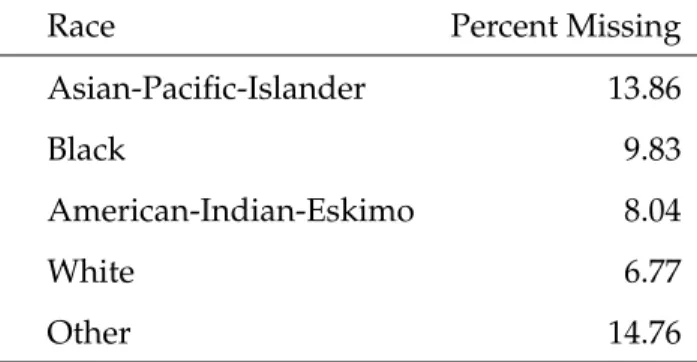
Most missingness is not completely at random. Often there are different factors that go into whether or not someone responds. One example, which comes from the “Adult” dataset (Section 2.4), shows the different non-response rates for different ethnicities. Table 1 shows the non-response rates in the occupation variable of the adult dataset based on race.
Table 1 shows that there is a higher non-response rate for “Asian-Pacific-Islanders” and “Other,” than for the remaining races. These rates show that these data do not have missingness
Table 1: Percent of Non-response Rates for Occupation Variable Based on Race in the "Adult" Dataset
Race Percent Missing
Asian-Pacific-Islander 13.86
Black 9.83
American-Indian-Eskimo 8.04
White 6.77
Other 14.76
completely at random, otherwise the percent missing would be more consistent across the entire dataset.
A variable is said to be missing at random if the probability of missingness depends only on available information. For the “Adult” dataset (Section 2.4), if work, education, marital status and the other variables are recorded for all people in the dataset, then occupation would be missing at random if the probability of non-response depended fully on the other recorded variables. Often, this is modeled as a logistic regression, with the outcome variable set as one for observed cases and zero for missing cases.
If the regression can control all variables in the dataset that affect the probability of missing-ness in the outcome variable, it is acceptable to exclude missing observations.
1.4.3 Missingness that Depends on Unobserved Predictors
If information has not been collected in the dataset, and this information affects the probability of missingness in the outcome variable, the outcome variable is no longer missing at random. For example, let’s assume in our “Adult” dataset (Section 2.4) that the probability of missingness in the
occupation variable was affected by type of work. Type of work is not a variable in our dataset, meaning it is an unobserved predictor. Occupation would not be missing at random, because its level of missingness depends on a variable we have not observed.
For datasets that contain missingness that is not at random, the missingness must be modeled. If not appropriately modeled, then there may be bias in the results.
1.4.4 Missingness that Depends on the Variable Itself
The most difficult type of missingness to deal with occurs when the probability of missingness depends on the actual missing value. An example of this situation would be if the missingness in the occupation variable from the “Adult” dataset (Section 2.4) depended on the occupation. If the people responding feel embarrassed about their jobs and chose not to answer the question, this would affect the probability of missingness for the occupation variable. The name for this situation is censoring, where the respondent censors their own responses, resulting in missingness in the data.
1.4.5 General Strategies for Missing Values
There are different approaches for dealing with missing values. The two most common approaches are using 1) complete cases and, 2) imputation. When using the complete cases approach, observations with any missing values are removed from the dataset, thus only cases with fully complete data are used. The second approach is to use imputation to fill in missing values.
have some serious drawbacks as well. Some problems with only using complete cases include:
1. Bigger standard error: Decreased sample size will lead to a bigger standard error for estimates.
2. Biased results: If data are missing at random, it means the cases with missing values are systematically different from the complete cases. This could bias the results.
3. Substantial data loss: If there are many missing values the number of complete cases could be small and most data will be discarded.
Imputation has its own benefits and drawbacks. The main benefit of imputation is that observed data can be kept (Janssen et al. 2010). You do not use imputation to make up or gain data, but the data that has been observed is not thrown away as with the complete case strategy. The power is stronger and standard error is decreased with the bigger sample size.
1.5 Structure of the Report
Section 2.1 and 2.2 describe two existing imputation methods and the two new methods are presented in Section 2.3. Section 2.4 briefly describes the datasets examined. Section 3 contains the results and Section 4 the conclusions.
2
Methods
2.1 Imputation within Random Forests
The R package randomForest has two built-in imputation methods to deal with missing values. One method uses the rough method (na.roughfix), and the other method uses the proximity matrix to impute values.
2.1.1 na.roughfix
The first approach in the R package randomForest is via the na.roughfix function. The underlying approach is considered to be a “rough-and-ready”" method. This method works one of two ways. If the variable being imputed is numeric, the median value of the imputed variable is chosen as the imputed value. If the variable being imputed is categorical, then the most common class of the variable that is being imputed is chosen as the imputed value. Thus the nickname rough-and-ready.
2.1.2 Proximity Matrix
When using the proximity matrix for imputation, the dataset with missing values is first imputed using na.roughfix (Ishioka 2013). Random forests is then run with the re-imputed dataset. A proximity matrix is created when running random forests, this matrix shows how similar observations are to each other. The proximity matrix will be of sizenxnbecause it compares how similar each observation is to all other observations. The(i,j)element of the proximity matrix is the
matrix, the missing values are then imputed for the missing data. For continuous variables, the values are imputed using the proximity-weighted average among non-missing values. Categorical variables are imputed using the category with the largest average proximity. The default is five iterations of re-imputation.
2.2 MICE
TheMiceR package (Buuren 2011) contains popular methods for imputation.Micestands for multivariate imputation by chained equations. The wayMiceframework is set up is to specify the imputation model on a variable basis to a set of conditional densities (Buuren 2011). The imputations are made through iterating over the conditional densities.
There are currently 22 different methods used for different situations with theMiceR package. The two methods used in this paper arePmm(predictive mean matching), and rf (random forest imputations). In R you specify the method used in theMice equation. For example thePmm function is called in R asmice(data,method=”pmm”), and for random forests inMicethe function
ismice(data,method = ”r f”). Pmmis the most commonly used method in theMiceframework.
The reasonPmmis so widely used is because it can be used for any type of data (not just numeric).
Micewith random forests is an imputation method built on theMiceframework (Shah et al. 2014). For continuous variables,Micewith random forests imputes the missing values by using random draws from independent normal distributions, centered on the means predicted from random forests. To obtain the estimator of the residual variance, “out-of-bag” mean square error is used. For categorical variables,Micewith random forests fits regression trees. For each missing value, a random tree is selected, and the prediction is imputed using that tree. In essence, it is
choosing between the categories with probability according to the mean random forest prediction.
2.3 New Imputation Methods
In this paper, we introduce two new imputation methods for random forests. They are both similar in their process, but with a change in how the missing data are originally imputed.
The algorithm for the new methods follows:
1. Temporarily remove the response variable, so the only variables remaining are the predictors.
2. Mark the predictors for whether or not they contain missing values, so it can be known which variable to predict for.
3. Impute all missing data by either using na.roughfix or with a random value sampled from the variable that contains missingness.
4. Set a variable that contains at least one missing value as the response variable.
5. Run random forests to find predictions for the missing values in the current response variable.
6. Fill in the missing values with the predicted values.
Steps 4, 5, and 6 of this new algorithm are performed for all variables as arranged in the data frame that contain missingness.
The difference between the two new methods is how the original dataset is imputed. One method uses na.roughfix from Section 2.1.1 to impute the dataset. The dataset is then completed with the median value (if numeric), or the most common value (if categorical). The other method
goes through the variable and selects a random value for the initial imputations. Throughout the results the two methods will be differentiated as New/Rough and New/Rand, where New/Rough used na.roughfix to complete the dataset and New/Rand has the data randomly filled.
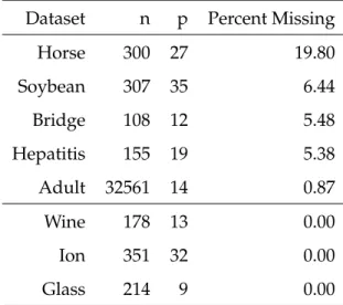
2.4 Datasets
All eight datasets used are found in the UC Irvine repository (Lichman 2013). Two types of datasets are used for comparison. Datasets that already contain missing values (assumed missing at random), and datasets where we introduce the missingness at random (missing completely at random).
Table 2: Description of Datasets Dataset n p Percent Missing
Horse 300 27 19.80 Soybean 307 35 6.44 Bridge 108 12 5.48 Hepatitis 155 19 5.38 Adult 32561 14 0.87 Wine 178 13 0.00 Ion 351 32 0.00 Glass 214 9 0.00
The datasets used in testing are “Horse”, “Soybean”, “Bridge”, “Hepatitis”, “Adult”, “Wine”, “Ion”, and “Glass”. The dimensions of these datasets are listed in Table 2. The “Horse” dataset
classifies whether or not a horse had surgery, based on health predictors of the horse. The “Soybean” dataset classifies which of 19 classes a soybean belongs to, based on predictors about the soybean and where it grew. The “Bridge” dataset classifies the type of bridge (out of six types of bridges in
Pittsburgh) ,based on predictors of the location and materials of the bridge. The “Hepatitis” dataset classifies whether or not someone with hepatitis died, based on health predictors of the person who has hepatitis. The “Adult” dataset classifies whether or not someone made over $50,000 per year, based on predictors of the person such as education, job, sex and others. The “Wine” dataset classifies the type of wine out of three possible classes, based on predictors for quantities of thirteen constituents found in the wine. The “Ion” dataset classifies whether or not there was structure in the ionosphere, based on predictors collected by a system in Goose Bay, Laboratory. The “Glass” dataset classifies the type of glass was used out of seven possible glasses, based on predictors of how much of different elements from the periodic table were contained in the glass.
3
Results
For our results, we compare the accuracy of six different imputation methods. The six meth-ods we used are: (1) New method with na.roughfix (New/Rough), (2) New method with random imputation (New/Rand), (3) random forests’ na.roughfix (Rough), (4) random forests’ proximity matrix (Prox), (5)Micewith random forests (Mice/For), and (6)MicewithPmm(Mice/Pmm). To make comparisons we complete the datasets using each of the methods, then run random forests on the completed dataset. We then find the percent correctly classified for each method.
The following results are from datasets that are either missing at random or missing com-pletely at random. For datasets that are missing at random, random forests is run on the imputed dataset to obtain the out-of-bag error rate. We then subtract the out-of-bag error rate from 1 and multiply by 100 to get the percent correctly classified (PCC).
For datasets that are missing completely at random, the datasets start complete and miss-ingness is introduced completely at random. The results show all six methods with six different percentages of missing data. Missingness is introduced at 10, 20, 30, 40, 50 and 60 percent missing-ness and each method is tested at these different levels. This gives us 36 combinations of methods and levels of missingness for each missing completely at random dataset. Tables 7, 9, and 11 have the percent correctly classified for each dataset at each level of missingness as well as a graph showing the effect of increased missingness.
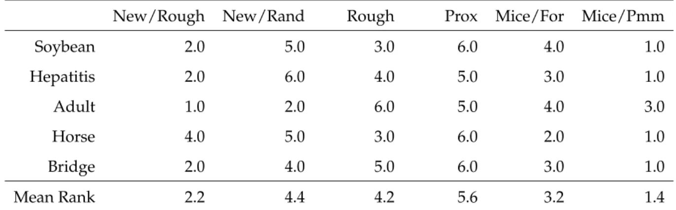
The first results come from datasets that are assumed to be MAR. Each method was run on each dataset with 100 repetitions. The PCC shown in the table is the mean PCC from the 100 repetitions. Table 3 gives the percent correctly classified for each of the six methods. Table 4 ranks each method by prediction accuracy, with rank = 1 for the most accurate method and rank = 5 for
the least accurate.
Table 3: MAR Datasets Percent Correctly Classified
New/Rough New/Rand Rough Prox Mice/For Mice/Pmm
Soybean 91.44 91.09 91.36 90.59 91.24 92.09
Hepatitis 86.19 84.46 84.83 84.76 85.92 86.21
Adult 79.90 79.87 79.68 79.69 79.79 79.80
Horse 76.69 75.93 77.06 74.63 77.58 78.55
Bridge 70.33 69.68 69.67 69.61 70.31 71.74
Table 4: Ranking for Each Method by Dataset
New/Rough New/Rand Rough Prox Mice/For Mice/Pmm
Soybean 2.0 5.0 3.0 6.0 4.0 1.0 Hepatitis 2.0 6.0 4.0 5.0 3.0 1.0 Adult 1.0 2.0 6.0 5.0 4.0 3.0 Horse 4.0 5.0 3.0 6.0 2.0 1.0 Bridge 2.0 4.0 5.0 6.0 3.0 1.0 Mean Rank 2.2 4.4 4.2 5.6 3.2 1.4
These results show that the most accurate method for data MAR is theMice with Pmm method. Our new method (New/Rough), where we first impute with na.roughfix, is the second most accurate method. This new method with roughfix consistently gives slightly better results for these MAR datasets than the current random forest imputation methods in almost every MAR test (Table 3). Except for the “Hepatitis” dataset, the difference is probably not of practical significance.
Each dataset for the missingness completely at random examples was randomly split into a test set and a training set. A test set is a dataset that is used only for predictions and is not used in creating the classifier. For running time purposes, different percentages of the datasets were used for training. For the wine, ion, and glass dataset 70%, 50% and 80% respectively were used as
the training set with the remaining used for the test set. PCC was found by first running random forest on the imputed training set and then predicting for the test set. Each method at each level of missingness was repeated 50 times, and the PCC is the mean percentage correctly classified from the 50 repetitions.
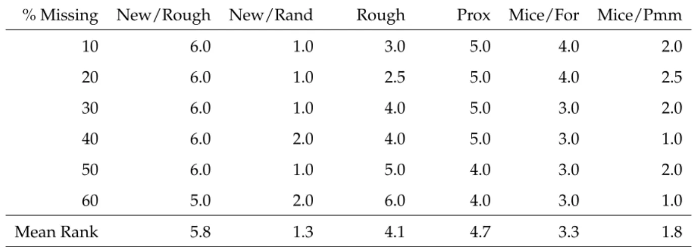
Table 5: Wine Dataset Percent Correctly Classified
% Missing New/Rough New/Rand Rough Prox Mice/For Mice/Pmm
10 96.29 97.42 96.67 96.33 96.50 96.88 20 95.96 97.38 96.96 96.38 96.83 96.96 30 95.25 97.04 95.62 95.54 95.88 96.42 40 94.92 95.96 95.38 95.12 95.62 96.33 50 93.08 95.42 94.21 94.54 94.83 95.38 60 92.12 93.96 91.62 92.75 93.54 95.21
Table 6: Ranking of Most Accurate Methods Wine Dataset
% Missing New/Rough New/Rand Rough Prox Mice/For Mice/Pmm
10 6.0 1.0 3.0 5.0 4.0 2.0 20 6.0 1.0 2.5 5.0 4.0 2.5 30 6.0 1.0 4.0 5.0 3.0 2.0 40 6.0 2.0 4.0 5.0 3.0 1.0 50 6.0 1.0 5.0 4.0 3.0 2.0 60 5.0 2.0 6.0 4.0 3.0 1.0 Mean Rank 5.8 1.3 4.1 4.7 3.3 1.8
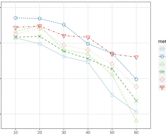
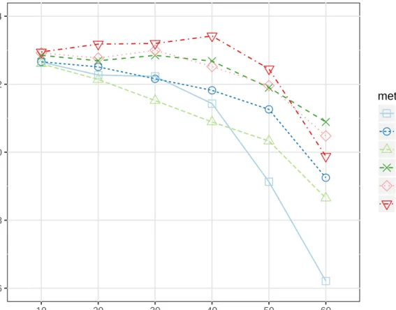
The datasets that are missing completely at random appear to fare differently depending on the dataset. For the wine dataset, Tables 5 and 6 show that the New/Rand method performed the best out of all six methods while New/Rough didn’t perform as well. In the ion dataset, Tables 7 and 8 show thatMicewithPmmwas most accurate and the two new methods were in the middle of the pack. Finally for the glass dataset, Tables 9 and 10 show that random forest’s
92 94 96 98 10 20 30 40 50 60 Percent Missing P
ercent Correctly Classified
method New/Rough New/Rand Rough Prox Mice/For Mice/Pmm
Figure 1: Performance of six classifiers for the wine dataset, based on the percentage missing.
Table 7: Ion Dataset Percent Correctly Classified
% Missing New/Rough New/Rand Rough Prox Mice/For Mice/Pmm
10 92.65 92.66 92.60 92.85 92.92 92.95 20 92.27 92.51 92.14 92.69 92.77 93.18 30 92.23 92.16 91.52 92.85 93.00 93.20 40 91.43 91.82 90.89 92.68 92.52 93.42 50 89.13 91.26 90.33 91.90 91.96 92.45 60 86.21 89.25 88.65 90.89 90.48 89.88
Table 8: Ranking of Most Accurate Methods Ion Dataset
% Missing New/Rough New/Rand Rough Prox Mice/For Mice/Pmm
10 5.0 4.0 6.0 3.0 2.0 1.0 20 5.0 4.0 6.0 3.0 2.0 1.0 30 4.0 5.0 6.0 3.0 2.0 1.0 40 5.0 4.0 6.0 2.0 3.0 1.0 50 6.0 4.0 5.0 3.0 2.0 1.0 60 6.0 4.0 5.0 1.0 2.0 3.0 Mean Rank 5.2 4.2 5.7 2.5 2.2 1.3 86 88 90 92 94 10 20 30 40 50 60 Percent Missing P
ercent Correctly Classified
method New/Rough New/Rand Rough Prox Mice/For Mice/Pmm
Table 9: Glass Dataset Percent Correctly Classified
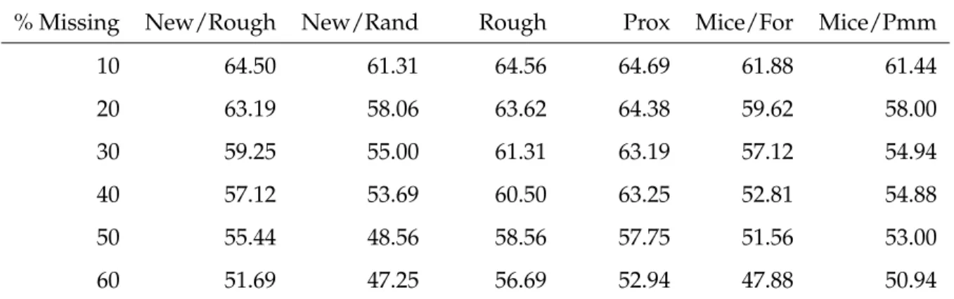
% Missing New/Rough New/Rand Rough Prox Mice/For Mice/Pmm
10 64.50 61.31 64.56 64.69 61.88 61.44 20 63.19 58.06 63.62 64.38 59.62 58.00 30 59.25 55.00 61.31 63.19 57.12 54.94 40 57.12 53.69 60.50 63.25 52.81 54.88 50 55.44 48.56 58.56 57.75 51.56 53.00 60 51.69 47.25 56.69 52.94 47.88 50.94
Table 10: Ranking of Most Accurate Methods Glass Dataset
% Missing New/Rough New/Rand Rough Prox Mice/For Mice/Pmm
10 3.0 6.0 2.0 1.0 4.0 5.0 20 3.0 5.0 2.0 1.0 4.0 6.0 30 3.0 5.0 2.0 1.0 4.0 6.0 40 3.0 5.0 2.0 1.0 6.0 4.0 50 3.0 6.0 1.0 2.0 5.0 4.0 60 3.0 6.0 1.0 2.0 5.0 4.0 Rank 3.0 5.5 1.7 1.3 4.7 4.8
45 50 55 60 65 10 20 30 40 50 60 Percent Missing P
ercent Correctly Classified
method New/Rough New/Rand Rough Prox Mice/For Mice/Pmm
proximity matrix (Prox) method performed the best, and the New/Rough method was the third most accurate method. Figures 1-3 give graphical representation of how each method performed at all levels of missingness for the “Wine,” “Ion,” and “Glass” datasets respectively. In each of the three Figures, the methods are all relatively close at the 10 percent level of missingness. As the level of missingness increases, the methods separate in their PCC. At the 60 percent level of missingness, the methods have separated significantly in their predictive abilities.
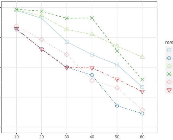
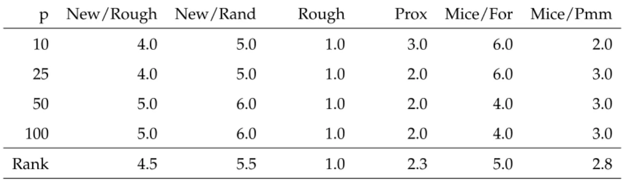
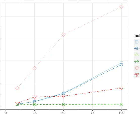
Another consideration when running any imputation method is the computational cost. The methods were timed using the microbenchmark R package (Mersmann 2015). Tables 11-14 show what happened as the number observations is increased, and then as the number of predictor variables is increased. The soybean dataset was used in testing. For Table 11, 50 observations were selected at random from the soybean dataset. For Table 13, a bootstrap sample of 500 was made from the soybean dataset. Predictor variables were bootstrap selected from the original soybean dataset. Table 11 gives us the time in seconds (using a mid-2012 Macbook Pro 2.5 GHz Intel Core i5) it takes to run each of the six methods with 50 observations while using 10, 25, 50, and 100 predictor variables. These results are only intended for relative performance. Table 13 gives us the time in seconds for the same number of predictor variables as above, but with 500 observations. We introduced 20 percent missingness to each dataset. Figure 4 graphically represents how each method performs with 50 observations and increased predictor variables. Figure 5 graphically represents how each method performs with 500 observations and increased predictor variables.
For all the different datasets, na.roughfix (Rough) is the fastest method by a large margin. The proximity method (Prox) is the second fastest method for all the datasets run. The other constant for all datasets is that theMicemethod with random forest (Mice/For) is the slowest method by a large margin. Both of the new methods take about the same amount of time to run at all levels of
Table 11: Times with Increasing Predictor Variables and 50 Observations (seconds) p New/Rough New/Rand Rough Prox Mice/For Mice/Pmm
10 0.34 0.33 <0.01 0.08 7.60 0.75
25 1.49 1.44 <0.01 0.12 29.93 3.59
50 5.36 5.14 <0.01 0.20 31.79 3.96
100 19.09 18.22 0.01 0.30 44.50 7.70
Table 12: Ranking of the Fastest Methods Increasing Predictor Variables with 50 Observations p New/Rough New/Rand Rough Prox Mice/For Mice/Pmm
10 4.0 3.0 1.0 2.0 6.0 5.0
25 4.0 3.0 1.0 2.0 6.0 5.0
50 5.0 4.0 1.0 2.0 6.0 3.0
100 5.0 4.0 1.0 2.0 6.0 3.0
Rank 4.5 3.5 1.0 2.0 6.0 4.0
Table 13: Times with Increasing Predictor Variables and 500 Observations (seconds) p New/Rough New/Rand Rough Prox Mice/For Mice/Pmm
10 5.33 5.35 <0.01 1.31 12.68 1.28
25 25.33 25.73 <0.01 1.87 27.58 2.99
50 96.57 98.80 0.01 2.94 55.71 6.07
100 342.62 355.83 0.01 4.74 77.49 8.56
Table 14: Ranking of the Fastest Methods Increasing Predictor Variables with 500 Observations p New/Rough New/Rand Rough Prox Mice/For Mice/Pmm
10 4.0 5.0 1.0 3.0 6.0 2.0
25 4.0 5.0 1.0 2.0 6.0 3.0
50 5.0 6.0 1.0 2.0 4.0 3.0
100 5.0 6.0 1.0 2.0 4.0 3.0
0 10 20 30 40 0 25 50 75 100 Number of predictors
Time (in seconds)
method New/Rough New/Rand Rough Prox Mice/For Mice/Pmm
Figure 4: Performance of six classifiers for datasets with an increasing number of predictor variables and 50 observations, based on time in seconds
0 100 200 300 0 25 50 75 100 Number of predictors
Time (in seconds)
method New/Rough New/Rand Rough Prox Mice/For Mice/Pmm
Figure 5: Performance of six classifiers for datasets with an increasing number of predictor variables and 500 observations, based on time in seconds
observations and predictors. Figure 4 shows that for a relatively small dataset, both of our new methods run at approximately the same speed and are relatively fast compared to theMicemethods, but they are considerably slower than the Rough and Prox methods. As we increase the number of predictors from 25 to 50 our new method becomes slower thanMicewithPmm(Mice/Pmm). Figure 5 shows that with the larger dataset with 500 observations, our new method is not faster thanMice withPmm(Mice/Pmm) at any level and becomes slower thanMicewith forest (Mice/For) between 25 and 50 predictors.
4
Conclusions
This paper proposes two new imputation methods based on a new algorithm. The methods are intended to improve percent correctly classified when predictors are imputed.
Out of the two new imputation methods, the new method with na.roughfix (New/Rough) appears to be the more accurate method. From our two new methods, New/Rough is the method out of the two that would be suggested to use.
For datasets that are missing at random, the new method with na.roughfix (New/Rough) performed better than all other methods exceptMicewithPmm(Mice/Pmm) against which it per-formed almost as well. For relatively small datasets the new method with na.roughfix (New/Rough) is faster than theMicewithPmm(Mice/Pmm) method. As the datasets get larger, the new methods both become slower than all other methods.
For datasets that have relatively small percentages of missing values, the imputation method may not make a significant difference in predictive ability. However, as the percent of missingness increases, the predictive ability in all six methods are significantly different.
There was not a consistent method that performed the best in all situations. It is suggested to try several different imputation methods and choose the most accurate method. This may not be practical in many situations, and so the suggested method to use generally isMicewithPmm. MicewithPmm(Mice/Pmm) was relatively consistent as the best method. Because it has been better optimized,MicewithPmm(Mice/Pmm) was relatively fast for large datasets and is the most accurate method to use to impute data, especially for large datasets.
forest imputation methods in terms of predictive ability. If computational speed is a primary concern, the existing native methods are currently much faster than the new methods as the number of predictors increase.
5
Future Work
Speed was a main factor in the new method (New/Rough) with na.roughfix (New/Rough). It was about as accurate as all other methods, but not as fast as the other methods, under certain conditions.
We plan on optimizing the new algorithm to perform faster. One way we could do this is to implement some of our code in C++. This will help to increase the speed in the loops, which is where the current speed breaks down.
Another improvement would be to run multiple imputations. For continuous variables, the missing value could be the mean value of the multiple imputations. For categorical variables, the missing value can be imputed multiple times and then the most common class can be imputed for the missing value.
We will also work to make the New/Rough method general enough that we can include it as a function in the randomForest R package.
References
Breiman, L. (1996), ‘Bagging predictors’,Machine Learning24(2), 123–140.
Breiman, L. (2001), ‘Random forests’,Machine Learning45, 5–32.
Buuren, S. V. (2011), ‘mice: Multivariate imputation by chained equations in R’,Journal of Statistical Software45, 1–67.
Gelman, A. & Hill, J. (2006),Data Analysis Using Regression and Multilevel/Hierachical Models, Cam-bridge University Press, New York.
Ishioka, T. (2013), Imputation of missing values for unsupervised data using the proximity in random forests,in‘The Fifth International Conference on Mobile, Hybrid, and On-line Learning’, The National Center for University Entrance Examinations, pp. 30–36.
James, G., Witten, D., Hastie, T. & Tibshirani, R. (2015),An Introduction to Statistical Learning (6th corrected printing), Springer, New York.
Janssen, K. J., Donders, A. R. T., Harrell, F. E., Vergouwe, Y., Chen, Q., Grobbee, D. E. & Moons, K. G. (2010), ‘Missing covariate data in medical research: to impute is better than to ignore’, Journal of Clinical Epidemiology63(7), 721–727.
Liaw, A. & Wiener, M. (2002), ‘Classification and regression by randomforest’,R News2(3), 18–22.
URL:http://CRAN.R-project.org/doc/Rnews/
Lichman, M. (2013), ‘UCI machine learning repository’.
URL:http://archive.ics.uci.edu/ml
Mersmann, O. (2015),microbenchmark: Accurate Timing Functions. R package version 1.4-2.1.
R Core Team (2016),R: A Language and Environment for Statistical Computing, R Foundation for Statistical Computing, Vienna, Austria.
URL:https://www.R-project.org/
Shah, A. D., Bartlett, J. W., Carpenter, J., Nicholas, O. & Hemingway, H. (2014), ‘Comparison of random forest and parametric imputation models for imputing missing data using mice: a caliber study’,American Journal of Epidemiology179(6), 764–774.