Substructured Systems
Li, G; Na, J; Stoten, DP; Ren, X
For additional information about this publication click this link.
http://qmro.qmul.ac.uk/jspui/handle/123456789/5999
Information about this research object was correct at the time of download; we occasionally
make corrections to records, please therefore check the published record when citing. For
more information contact [email protected]
Adaptive Neural Network Feedforward Control for
Dynamically Substructured Systems
Guang Li, Member, IEEE, Jing Na, David P. Stoten, and Xuemei Ren
Abstract— The potential applications of dynamically tured systems (DSSs) with both numerical and physical substruc-tures can be found in diverse dynamics testing fields. In this paper, an adaptive feedforward controller based on a neural network (NN) is proposed to improve the DSS testing perfor-mance. To facilitate the NN compensation design, a modified DSS framework is developed so that the DSS control can be considered as a regulation problem with disturbance rejection. Then an adaptive NN feedforward compensation technique is proposed to cope with uncertainties and nonlinearities in the DSS physical substructure. The proposed NN technique generalizes the existing results in the literature, and it does not require any information of the plant model and disturbance model, which significantly simplifies its application on DSS. In particular, we propose a novel adaptive law for the NN online learning, where appropriate NN weight error information is derived and used to achieve improved performance. Real-time experimental results on a mechanical test rig demonstrate the improved performance by using the NN compensation strategy and the new adaptation law.
Index Terms— Adaptive control, dynamics testing, mechanical system, neural networks (NN).
I. INTRODUCTION
T
HE dynamically substructured system (DSS) technique is currently receiving significant attention in various fields, e.g., large-scale structural and automotive system testing. A DSS contains both numerical and physical substructures [1]. In a DSS test, a full-size system is decomposed into two or more substructures, in which only the critical parts (usually containing nonlinearities and uncertainties) are tested phys-ically, while the remaining parts (usually containing large-scale components) are tested simultaneously in numerical model form. In this sense, DSS is able to test full-size criticalManuscript received November 26, 2012; revised March 22, 2013; accepted May 31, 2013. Manuscript received in final form June 20, 2013. This work was supported in part by the U.K. Engineering & Physical Sciences Research Council under Grant EP/D036917, the National Natural Science Foundation of China under Grant 61203066 and Grant 61273150. Part of this paper was presented at the 18th IFAC World Congress 2011, Milan, Italy. Recommended by Associate Editor F. Chowdhury.
G. Li is with the Department of Mechanical and Nuclear Engineering, the Pennsylvania State University, University Park, PA 16802 USA (e-mail: [email protected]).
J. Na is with the Department of Mechanical and Electrical Engineering, Kunming University of Science and Technology, Kunming 650093, China (e-mail: [email protected]).
D. P. Stoten is with the ACTLab, the Department of Mechani-cal Engineering, University of Bristol, Bristol BS8 1TR, U.K. (e-mail: [email protected]).
X. Ren is with the School of Automation, Beijing Institute of Technology, Beijing 100081, China (e-mail: [email protected]).
Color versions of one or more of the figures in this paper are available online at http://ieeexplore.ieee.org.
Digital Object Identifier 10.1109/TCST.2013.2271036
components of an emulated system in a laboratory environ-ment so that the drawbacks involved with purely numerical and purely physical testings can be avoided. The applications of the DSS concept can be found in areas, such as automotive [2], aerospace [3], civil engineering [4]–[6], and robotics [7]. See [1] and [8] for a detailed discussion on the advantages of using DSS.
DSS is distinguishable from the hardware-in-the-loop (HIL) method, which is used traditionally to test the performance of a controller, with a hardware interface to an embedded numerical plant. However, in more recent developments, the HIL approach has some common features with DSS method-ology [9]. The distinguishing feature of DSS is the synthesis of a composite system involving both numerical and physical testing components, which must be synchronized at their interfaces to create a similar testing environment to the original emulated system. See [2] for a discussion about the differences between the concepts of DSS and HIL.
In a DSS test, it is expected that the differences between the salient responses of the DSS and the original emulated system are as small as possible. These differences are affected by the synchronization of the physical and numerical substructures. Hence, the control design objective in a DSS test is to synchronize the interaction signals at the interface between the numerical and physical substructures subject to the testing (i.e., excitation) signal. In [1], a substructuring framework and general control design methodologies were proposed and successfully applied to a quasi-motorcycle (QM) DSS test rig [10], [11].
Generally, the performance of a DSS test can be influenced by two factors. One factor is from the inevitable and significant uncertainties and nonlinearities in the physical substructure. Ignoring these problems during DSS controller designs may greatly deteriorate the testing results. Because of this reason, a DSS usually requires a high fidelity controller which must be able to cope with uncertainties and nonlinearities in the physi-cal substructure. Some DSS control strategies are proposed to overcome these problems in different situations. Among these strategies, an adaptive control algorithm, called minimum control synthesis, is demonstrated to be an effective control method for DSS control problem [12], [13]. The second factor is the complication introduced by the dynamics of the actuators employed in a DSS. The limiting characteristics of the actuators can significantly deteriorate the DSS performance in some cases. These effects are explicitly compensated out by the design given in [1]. So-called actuator delay compensation is investigated by [14]; the actuator saturation problems in DSS control were addressed in [15]–[18].
In this paper, we focus on the first factor influencing the DSS performance by employing neural network (NN) feedforward compensation technique. This is motivated by the approximation capability of NN in identification and control design, which is widely studied in the control community [19]–[25]. There are also several results dedicated to NN feedforward compensation for the rejection of disturbances [26], [27]. Recently, Ren et al. [28], [29] developed two novel NN feedback-feedforward control schemes to attenuate the effect of external vibrations on nonlinear mechanical systems, in which the closed-loop stability can be guaranteed in the sense of Lyapunov. In addition, the dynamical models of the plant, disturbance and sensors are not required, while only the accelerometer measurements of disturbances are utilized, which makes them attractive from a practical viewpoint. In these results, the NN weights are updated online adaptively, and e-modification [20], [21] is introduced to guarantee the boundedness of adaptive parameters. It is noted that NN adaptive techniques are rarely utilized in the DSS system design and synthesis.
In this paper, we will investigate a novel DSS control strategy: an adaptive controller with NN feedforward compen-sation, and propose a novel adaptive law for online NN weight learning to improve the convergence performance [30]. We first transform the existing generalized DSS framework in [1] into a modified framework, and then the DSS control design can be considered as a regulation problem with measured disturbance rejection. With this observation, an adaptive NN compensator can be designed and superimposed upon a pre-designed linear two degree-of-freedom (DOF) DSS controller to achieve improved synchronization. The linear feedback controller is employed to guarantee the stability of the closed-loop system, while the NN is used to provide an extra feedforward compensation action to cope with uncertainties and nonlinearities. The salient feature of the proposed method lies in the fact that the NN feedforward control design does not require any information on the plant, and the effect from the system modeling uncertainties can also be diminished through the NN feedforward compensation. The experimental results on a QM DSS test rig demonstrate the superior performance of applying NN feedforward compensation over a linear feed-forward controller alone. The NN compensation strategy in [28], [29] was also generalized from single input, single output (SISO) case to generic multiple input, multiple output (MIMO) cases, which makes it possible to apply this strategy to the coupled multivariable DSS control problem. In particular, in contrast to our previous work [31], we also propose a novel adaptive law for NN weight learning beyond the conventional
e-modification orσ-modification [20], [21], where appropriate
weight error between the ideal weights and their estimation is derived and used to update the NN weights so as to further improve the overall performance.
The structure of this paper is as follows. We start with a generalized DSS framework for control system design in Section II. In Section III, we first transform the generalized DSS framework to an alternative framework, and then address the details of the design of the NN compensator based on this transformed DSS framework. In Section IV, the DSS test rig
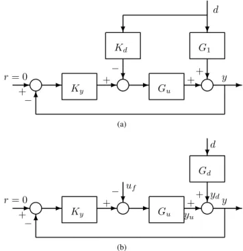
Fig. 1. Linear control DSS framework of [1].
and the real-time experimental results are presented. Finally, the paper is concluded in Section V.
II. GENERALIZEDDSS CONTROLFRAMEWORK AND THE
QM TESTRIG
A. Generalized DSS Control Framework
The general DSS framework proposed in [1] was shown in Fig. 1. In this framework, the three terms {G0,G1,G2}
are used to represent a generalized system, yielding the generalized substructures1 and 2, together with the
gen-eralized outputs z1,z2. For a class of practical applications,
we can denote 1 as the numerical substructure and 2
as the physical substructure, respectively, hence 1 = N and 2 = P. The following associations can also be made: G1 is related to N, G0 to both P and N, and
G2 to the so-called transfer system component of P. The transfer system consists of the test specimen actuators, sensors and mechanical support structure. In the figure, {d,u} are external excitations and the DSS control signals, while{z1,z2}
are the outputs of the numerical and physical substructures, respectively.
In the DSS test, the two outputs must be in near-perfect synchronization; that is, the substructuring error y:=z1−z2
must always be driven toward zero if a DSS is to function satisfactorily. The control objective of the DSS, as shown in Fig. 1, is thus to minimize the DSS error, i.e., the difference between z1and z2
y=z1−z2=G1d−G0u−G2u (1)
using a control signal u produced by a 2-DOF controller
u=Kdd+Kyy (2) where Kdis a linear feedforward controller and Ky is a linear feedback controller.
Under this DSS framework shown in Fig.1, various DSS controllers can be designed to achieve the control objective. A straightforward design for the feedforward linear controller
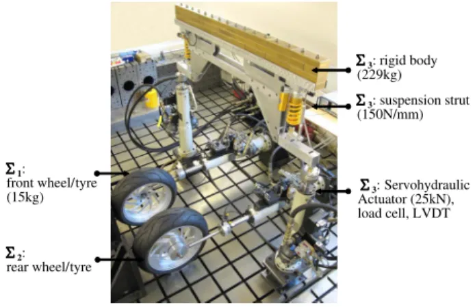
Fig. 2. Photograph of the quasi motorcycle test rig.
is to choose Kd =(G0+G2)−1G1and Kyvia pole-placement, as shown in [1].
However, this ideal situation can never be perfectly real-ized due to parameter variations, unmodeled dynamics and unknown external disturbances in practical systems. In this paper, we present a new method that uses NN to provide an extra compensation to mitigate against the above effects. A case study is used to demonstrate the effectiveness of this method.
B. QM Test Rig and Its Substructured Form
In this case study, we apply our control strategy (to be pre-sented later) to a QM hydraulically actuated system developed at the University of Bristol; see Fig. 2 for a photograph of the rig and Fig. 3 for its schematic representation. This test rig was extensively studied in the previous work [11]. Here, we briefly introduce it again for completeness.
The test rig is composed of three subsystems, the first of which is a rigid vehicle body with an evenly distributed mass of 229 kg, and two suspension struts together with two swing arms. Each suspension strut is connected to the vehicle body at one end and to a swing arm at the other end. Two 25-kN hydraulic actuators are attached to the swing arms, respectively. The second and third subsystems consist of two separate 25-kN hydraulic actuators, attached to the hubs of the front and rear wheels/tires. Each hydraulic actuator has a built-in lbuilt-inear variable differential transformer for the measurement of displacement and also a load cell for the measurement of force. For test purposes, we can select each subsystem either as a numerical or a physical element. Hence, we can derive different DSSs for this test rig, which are classified according to the type of forces at the interfaces between the subsystems [11].
In this paper, we only focus on one scenario: the QM body with the two suspension struts constitute the physical sub-structure, while the front and rear wheels form the numerical substructure. We call this a single mode (SiM) substructure since only one type of force, comprised of inertial terms, is imposed on the physical substructure. The interface variables are the displacements and the forces at the attachment points of the wheel hubs and the ends of the swing arms and they are represented, respectively, as{y31,y32},{y1,y2},{f31, f32}
and{f1, f2}, see Fig. 3.
Fig. 3. Schematic representation of the quasi motorcycle test rig. (a) Vehicle body with two suspension struts and two swing arms. (b) Hub and wheels with j=1 for the front and j=2 for the rear.
TABLE I
NOTATIONLIST FOR THEQM SYSTEM–VARIABLES
The dynamical equations of the QM system can be found in [11], and the linearized equations of motion after the Laplace transformation is summarized as follows:
y1=Gyd1d1−Gy f 1f1 (3) y2=Gyd2d2−Gy f 2f2 (4) f31= P2s2yb31+P3s2yb32 (5) f32= P3s2yb31+P1s2yb32 (6) yb31=G31y31 (7) yb32=G32y32 (8) with Gyd1= c1s+k1 m1s2+c1s+k1 Gyd2= c2s+k2 m2s2+c2s+k2 Gy f 1= 1 m1s2+c1s+k1 Gy f 2= 1 m2s2+c2s+k2 G31= c31s+k31 m31s2+c31s+k31 G32= c32s+k32 m32s2+c32s+k32 P1= m3L21 L2 + J3 L2 P2= m3L22 L2 + J3 L2 P3= m3L1L2 L2 − J3 L2 with m31 =m3L1/L and m32 =m2L2/L.
Here all the variables and parameters, with their nominal values, are listed in Tables I and II.
Suppose the forces {f31,f32} are chosen as the interface
TABLE II
NOTATIONLIST FOR THEQM SYSTEM–PARAMETERS
synchronizing signals, which are generated by the action of the inner-loop controlled actuators
y31=GAy1u31 (9)
y32=GAy2u32 (10)
where the displacement output transfer functions
GAy1 =GAy2= 43.6
s+37.6
are the dynamics of the actuators and they are derived by system identification.
By manipulations of (3)–(8), the SiM can be represented by the DSS framework of Fig. 1 with
z1= y1 y2 z2= y31 y32 d= d1 d2 u= u31 u32 and G1=Gd G0=GIGA G2=GA where Gd = Gyd1 0 0 Gyd2 GA = GAy1 0 0 GAy2 GI = Gy f 1P2s2G31 Gy f 1P3s2G32 Gy f 2P3s2G31 Gy f 2P1s2G32 .
III. ADAPTIVEDSS CONTROLWITHNN COMPENSATION
In this section, we will first transform the generalized DSS framework (as shown in Fig. 1) into a regulation form and then we will develop a novel adaptive control scheme with NN feedforward compensation.
A. Adaptive NN Feedforward Control Framework for DSS System
Substituting (2) into (1) leads to
y= [I+GuKy]−1Gdd (11) where
Gu:=G0+G2 Gd:=G1−GuKd.
Fig. 4. Equivalent representations of Fig. 1. (a) Framework 1. (b) Frame-work 2.
According to [11], Fig. 1 can be transformed into an equivalent framework as shown in Fig. 4(a), which can be further trans-formed to an equivalent alternative framework in Fig. 4(b). In Fig. 4(b), Gd contains a predesigned feedforward controller
Kdand denotes the disturbance model from d to the output y. If the testing signal d is assumed to be the external disturbance, and the reference r is set to zero (r =0), the control problem in Fig. 4(b) amounts to a standard regulation control problem with measured disturbance rejection, i.e., to regulate the output
y in Fig. 4(b) to zero under the disturbance d. If we choose Kd=G−u1G1, as shown in Section II, then y ≡0. However,
this can never happen due to unmodeled uncertainties. Hence
uf is added as an extra feedforward control signal, which is generated by a compensator to attenuate the extra disturbance that cannot be fully compensated by Kd = G−u1G1 (i.e.
Gd=0 due to the modeling errors).
Following the similar arguments for choosing
Kd, if we can design an ideal compensator as
u∗f = Gfd = Gu−1Gdd, then it is intuitively reasonable that the effect of the disturbance d can be eliminated completely in the nominal case. However, this inverse-based feedforward controller may not be feasible in practical applications. On the one hand, the inverse of Gu may not be derived in a straightforward manner if it is nonminimum phase or noninvertible; on the other hand, when the system nonlinearities and uncertainties are significant, the performance can significantly degrade. For this reason, we aim to use the nonlinear NN compensation technique to construct the feedforward compensator, so that the previously mentioned problems can be avoided.
Although a predesigned feedback control Kd is used in Fig. 4 (Kd is incorporated into Gd), it should be noted that the NN design does not depend on the existence of
Kd, i.e., in the worst case, we can set Kd = 0, so that the feedforward compensation uf is used to accommodate
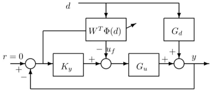
Fig. 5. DSS control with NN compensation.
all unknown dynamics and disturbances without using the disturbance model. Thus, the subsequent analysis is still valid for Kd=0.
The following development is based on the transfer function matrix from the signals d and −uf to y:
GC L:=
(I+GuKy)−1Gd, (I+GuKy)−1Gu
whose state space realization is
˙
x=Ax+Bu(−uf)+Bdd, y=C x (12) where x ∈ Rnx, y ∈ Rny, u
f ∈ Rnu, d ∈ Rnd, and
A,Bu,Bd,C are system matrices with appropriate dimen-sions. Note that GC L is strictly proper by assuming that G0,
G1and G2 are also strictly proper.
As this paper mainly focuses on the feedforward compen-sator design and synthesis, the predesigned linear controllers
Ky and Kd are assumed to stabilize the closed-loop system without disturbance. In this paper, a linear quadratic regulation (LQR) control will be used to design the linear controllers as shown in Section IV-A. To facilitate further analysis, the following assumption must hold.
Assumption 1: The linear control DSS framework in Fig. 1
(or equivalently, Fig. 4) is asymptotically stable.
Remark 1: In the nominal case, Assumption 1 can be
satisfied by appropriately designing the stabilizing linear con-trollers Ky and Kd (See Section IV-A for example). Assump-tion 1 guarantees that A in (12) is Hurwitz. Hence, there exist positive definite matrices P and Q such that ATP+P A= −Q
holds. This condition will be used later in the proof of the closed-loop stability involving the NN compensator.
Based on the transformed DSS framework in Section III-A, we can now design the NN compensator for DSS. If we use an auxiliary external disturbance ω to represent the effects of uncertainties and nonlinearities on the DSS dynamics, then (12) can be modified as
˙
x=Ax+Bu(−uf)+Bdd+ω, y=C x (13) where y is the DSS error to be regulated. To compensate for this extra disturbance ω and also d on the DSS error
y, the adaptive DSS control scheme with a feedforward NN
compensator (as shown in Fig. 5) is proposed.
It is proved that an unknown function can be approximated by an NN in a compact set [20]. Then we can use an NN to approximate the dynamicsu˜∗f :=ω+Bdd ∈Rnx as
u∗f :=W∗T(d)+φ (14)
such that
˜
u∗f =Buu∗f. (15) Here Bu,Bd are known matrices defined in (12); W∗ ∈
RN×nu, with N >0, is the optimal network weighting matrix;
φ ∈ Rnu is the approximation error vector. The following
assumption holds for the NN adaptive laws to be presented.
Assumption 2: The optimal NN weighting matrix W∗
and the approximation error vector φ are bounded by
W∗ ≤WN,WN >0 andφ ≤ε, ε >0.
The feedforward compensation signal uf is provided by
uf =WT(d) (16) where W ∈ RN×nu is the adaptive NN weight matrix,
(d) = [S1(d),S2(d),…,SN(d)]T ∈ RN is the network basis function; Si(d)is sigmoidal functions with the form of
Si(d)= (a/1+e−bd)−c, where a,b ∈ R+ and c ∈ R are NN tuning parameters that represent the bound, slope and bias of the sigmoidal curve, respectively.
Substituting (14), (15), and (16) into (13) with an NN compensation can be expressed as follows:
˙
x=Ax+BuW˜T(d)+Buφ, y=C x (17) whereW˜ =W∗−W is the NN weight error.
Remark 2: In the DSS synthesis, the external excitation d is
precisely known and available. However, the proposed method can also be extended to a system (not the DSS case) in which only an approximated measurement of d is available (e.g., the accelerometer signal of d as in [28]). In addition, the established feedforward control does not depend on the system model and the disturbance model, which can simplify the DSS control system design when the system model (especially for the physical substructure) cannot be easily derived.
Remark 3: In the proposed DSS framework in Fig. 5, the
NN compensator is superimposed on a predesigned linear feedforward controller Kd to provide an extra compensation signal in the feedforward path, so that the uncertainties and nonlinearities in the plant can be compensated. Hence, this method can guarantee a better performance than the case with linear feedforward controller alone. This is also different to the method proposed by [29], where only an NN compensator without a linear feedforward controller is employed.
B. Adaptive Law Design With e-Modification
In this subsection, we first present an adaptive law for updating the NN weights based on the e-modification [20]. The NN weight W of (16) can be updated [31] based on
˙
W = {(d)yTFT −σyW} (18) whereyis the Euclidean norm of the output y; = T >0 is the adaptive learning matrix with ∈ RN×N; σ > 0 is the e-modification parameter and F ∈ Rnu×ny is a designed
matrix fulfilling the matching condition P Bu =CTFT. This condition will be utilized in the proof of the closed-loop stability [see (20)]. Note that this matching condition is usually considered as the strictly positive real type condition, which can be fulfilled in our DSS study. A detailed analysis for the
construction of matrices F and Q can be found in [32] to satisfy this condition.
We have the following result.
Theorem 1: Consider the DSS dynamics described by (13)
with the NN feedforward control (16) and the parameter update law (18), the system states and the network weight error are uniformly ultimately bounded (UUB).
Proof: Consider the following Lyapunov function: V = 1 2x T P x+1 2tr{ ˜W T −1W˜} (19)
where tr{·}is the trace of the corresponding matrix.
By applying (17) and Assumptions 1, 2, we can obtain the time derivative of V as follows:
˙ V = 1 2x T( ATP+P A)x+xTP Bu ×{W∗T(d)+φ−WT(d)} +tr{ ˜WT −1W˙˜} = −1 2x T Qx+xTP Buφ+yTFTW˜T(d) −tr{ ˜WT(d)yTFT −σy ˜WTW}. (20) Since tr{ ˜WT(d)yTFT} = yTFTW˜T(d)and tr{ ˜WTW} = tr{ ˜WT(W∗− ˜W)} ≤ −( ˜W −12WN)2+14WN2, it follows that ˙ V ≤ −1 2Qmx 2−σC Mx( ˜W − 1 2WN) 2 +PMBMεx +σ CMx 4 W 2 N ≤ −x{1 2Qmx +σCM( ˜W − 1 2WN) 2 −PMBMε−σ CM 4 W 2 N} (21)
where PM, BM and CM are the maximum eigenvalues of
P, Bu and C respectively, and Qm is the minimum eigenvalue of Q.
It can be shown that V˙ ≤0 as long as either
x ≥2(PMBMε)+ σCM 2 W 2 N Qm (22) or ˜W ≥ 1 2W 2 N+ PMBMε σCM + WN2 4 . (23) Therefore, V is negative outside a compact set defined by˙
(22) and (23) in the x and ˜W plane, which is shown to be an attractive set for the system. According to the Lyapunov theorem extension [20], this demonstrates the UUB [20], [21] of both the system state x and the NN weight error ˜W. This means that the regulation performance of the system of Fig. 5 can be retained and the system output y is bounded in a small neighborhood around zero. In this case, the synchronization of the DSS control can be achieved.
C. Adaptive Law Design With Parameter Error
To guarantee the stability of system (17), adaptive law (18) is proposed, for which the first term is the gradient-based error and the second termσyW is the e-modification term
[20], which is employed to guarantee the boundedness of NN weights W . However, the introduction of such a term may degrade the adaptive learning speed. As known in adaptive control literatures, the parameter adaptation should preferably include some information on the parameter estimation error to improve the error convergence [30].
In this subsection, we will further investigate a novel adaptive law for NN weight learning, which is driven by the tracking error and the appropriate parameter error. To do this, a set of auxiliary system variables are first derived by intro-ducing appropriate filter operations on the system dynamics so that the NN weights error information is obtained explicitly and used for NN weights learning. The novel adaptive law is incorporated into the feedforward NN control implemen-tation and the closed-loop stability will also be proved. The introduction of such a term in the adaptation allows for fast learning speed and thus better control performance. This is clearly different to previous work [31].
To derive the NN weights error, we consider error system (17) and define the filtered variables of x and as
kx˙f +xf =x, xf(0)=0 (24a)
k˙ f +f =, f(0)=0 (24b) where k>0 is a filter parameter.
Then the following fictitious filter defines the auxiliary variableφf:
kφ˙f +φf =φ, φf(0)=0 (25) and the filtered version of system (17) can be derived as
˙
xf =Axf +BuW˜Tf(d)+Buφf
=Axf +Bu(W∗−W)Tf(d)+Buφf
(26)
where xf ∈ Rnx, φf ∈ Rnu and φf ∈Rnu are the filtered variables of x , φ and φ, respectively. Note thatφ is not precisely known, and the filter operation (25) and the associate variableφf are only used for analysis.
It can be obtained from (24)–(26) that
˙ xf = x−xf k (27a) x−xf k −Axf =Bu(W ∗T − WT)f +Buφf. (27b) Now we introduce another auxiliary filtered matrix variables
L(t)∈RN×N and Q(t)∈Rnx×N as ˙ L(t)= −l L(t)+fTf (28a) ˙ Q(t)= −l Q(t)+ [(x−xf)/k−Axf +BuWTf]Tf (28b) where l >0, and the initial conditions L(0)=0, Q(0)=0. One may obtain the solutions of (28) as
L(t)= t 0 e−l(t−τ)f(t)Tf(t)dτ (29a) Q(t)= t 0 e−l(t−τ)[(x−xf)/k−Axf+BuWTf]Tf(t)dτ. (29b)
Then we define a matrix variable M(t)∈Rnx×N by
M(t):=BuWTL(t)−Q(t) (30) where the matrix variables L(t)and Q(t)are determined by the differential equation (28).
Substituting (27) and (29) into (30) gives
M(t)= −BuW˜TL(t)−ζ(t) (31) whereζ(t):=0te−l(t−τ)BuφfTf(τ)dτ, andζ is bounded by ζ ≤εζ for someεζ >0 since the NN basis vectorf and the approximation errorφf are all bounded.
With the above development, we introduce another novel NN adaptive law for feedforward control (16) as follows:
˙
W = [(d)yTFT −σMTBu] (32) where ∈ RN×N, σ ∈ R are being positive learning gains
>0, σ >0.
Remark 4: Comparing (32) with (18), one can find that the
second term is different. As shown in (31), the variable M derived from (30) denotes the information on the NN weights errorW , which is then used to drive the adaptation. Therefore,˜
faster learning speed is expected. In addition, similar to [30], we can prove that the matrix L(t)in (29) is positive definite (i.e. L(t) > β >0) provided the persistent excitation (PE) of matrix holds. Since f is the filtered version of based on (24),f is PE as long asis PE, i.e.,
t
0f(t)
T
f(t)dτ > 0, and thus L(t) = 0te−l(t−τ)f(t)Tf(t)dτ > 0 is true. This can be achieved in our DSS system with external distur-bance d.
The following theorem demonstrates the stability of using this adaptive law.
Theorem 2: Consider the DSS described by (13) with the
NN feedforward control (16) and the parameter update law (32). The system states x and the network weight errorW are˜
all uniformly UUB.
Proof: Consider the Lyapunov function candidate V =1 2x T P x+1 2tr{ ˜W T −1 ˜ W}. (33) The first derivative of V along (17) and (31) is
˙ V = −1 2x TQx+xTP B uφ+σtr{ ˜WTMTBu} = −1 2x T Qx+xTP Buφ −σtr{ ˜WTLTW B˜ uTBu} −σtr{ ˜WTζTBu} ≤ −1 2x T Qx+xTP Buφ−σc1 ˜W2+σc2 ˜W (34)
where c1 = βBm2 > 0,c2 = εζBM > 0 are all bounded constants, where Bm is the minimum eigenvalue of Bu.
By applying the Young’s inequality ab ≤ a2/c+cb2 for
c>0 on the terms xTP B
uφand c2 ˜W, it follows that
˙ V ≤ − 1 2(Qm−2c)x 2+(PMBMε)2 c −σ(c1−c) ˜W2+σ c22 c ≤ −γV +θ (35)
where γ = min(Qm−2c)/PM,2σ(c1−c)/ −M1 and θ =
(PMBMε)2/c+σc22/c are all positive constant if we select
c<min(Qm/2,c1). Then according to the Lyapunov theorem
extension [20], the UUB of both the system states x and the NN weight errorW are all guaranteed.˜
Remark 5: In [28], [29] only second-order SISO or
decoupled MIMO systems were considered. Here, The-orem 1 extends the results to high-order multivariable systems, and more specifically, this paper incorporates the NN feedforward compensation into a modified DSS control framework to propose a DSS control synthesis methodology.
Remark 6: In the practical implementation of the
pro-posed NN compensation (16), the form of the feedfor-ward control neural network WT(d)can be converted into a discrete-time version in which the input vector of the NN at the sampling time k can be selected as (d) =
[S(d(k)),S(d(k−1)),…,S(d(k−N))]. This was practically verified by [29] and others in the study of steady-state performance.
Remark 7: The adaptive NN compensation technique
pro-posed in this paper is effective in coping with uncertainties present in a DSS. In some practical DSS testings, con-straints may also be a prominent problem to be resolved. When both constraints and uncertainties are predominant in a DSS testing, it is possible to combine the anti-windup compensation technique in [17], [18] with the NN algorithm proposed in this paper to cope with these problems at the same time.
IV. EXPERIMENTALRESULTS
A. Control System Design
For the DSS shown in Section II, the linear feedback controller Ky and a linear feedforward controller Kd are designed using an LQR strategy to fulfill Assumption 1.
Suppose that the transfer functions G0(s), G1(s)and G2(s)
are strictly proper and their state space matrices are Gi(s)∼
(Ai,Bi,Ci,0)with i =0,1,2. Then, according to the DSS framework shown in Fig. 1, the state space realization for the whole system can be written as
˙ x = ¯Ax+ ¯Buu+ ¯Bdd (36a) y= ¯C x (36b) with x=x0T x1T x2TT ∈Rnx and ¯ A= ⎡ ⎣A0 A0 01 00 0 0 A2 ⎤ ⎦ ¯ Bu= ⎡ ⎣B00 B2 ⎤ ⎦ ¯ Bd= ⎡ ⎣B01 0 ⎤ ⎦ ¯ C=−C0C1−C2 .
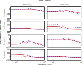
−200 −100 0 From: In(1) To: Out(1) −360 0 360 720 To: Out(1) −100 −50 0 50 To: Out(2) 100 105 −360 0 360 720 To: Out(2) From: In(2) 100 105 Bode Diagram Frequency (rad/s)
Magnitude (dB) ; Phase (deg)
Fig. 6. Bode plots of (solid lines) Ky(s)and (dashed lines) Kd(s). The top left two plots are the gain and phase of Ky11 and Kd11; the top right two plots are the gain and phase of Ky12and Kd12; the bottom left two plots are the gain and phase of Ky21and Kd21; and the bottom right two plots are the gain and phase of Ky22and Kd22.
The corresponding equations for a linear observer (for the theoretical details of the design of LQR and linear observer, see [33] are
˙ˆ
x= ¯Axˆ+ ¯Buu+ ¯Bdd+L(y− ˆy) (37a)
ˆ
y= ¯Cxˆ. (37b)
Suppose the feedback gain K is computed from the alge-braic Ricatti equation so that
u = −Kxˆ. (38) Substituting (38) and (37b) into (37a) leads to the controller-observer equations
˙ˆ
x=(A¯−LC¯− ¯BuK)xˆ+ ¯Bdd+L y (39a)
u= −Kxˆ. (39b)
Therefore, the feedback controller is Ky ∼(Ac,Bc,y,Cc,0) and the feedforward controller is Kd ∼ (Ac,Bc,d,Cc,0), where
Ac= ¯A−LC¯− ¯BuK, Bcd = ¯Bd
Bc,y =LCc= −K.
The weights of the Kalman filter when designing the observer are chosen as Qn = Iny and Rn = 0.25×Inu; the
weights for the algebraic Ricatti equation are Q = ¯CTC and¯ R=0.01×Inu. With these parameters, the constant feedback
gain K can be calculated by the MATLAB routinelqr. The bode plots of Ky and Kd are shown in Fig. 6.
We design both NN feedforward compensators using the adaptive laws (18) corresponding to Theorem 1 and (32) corresponding to Theorem 2. A single-layer NN with 4 neurons is employed in both NN compensators. The number of neurons is selected by gradually increasing this number until no further improvement of regulation performance can be observed, while the computational costs are also taken into consideration in the experiments. The network basis functions for both NN compensators are the same and takes the form of (d) = [(di(k)), (di(k−1)), (di(k−2)),
Fig. 7. Comparison of DSS errors (y1) when controlled by (a) LQR alone, (b) LQR with NN compensator from Theorem 1, and (c) LQR with NN compensator from Theorem 2.
(di(k−3))]T, where the sigmoidal functions are tuned as
S(di)=(2/1+e−0.01di)−0.1; here diis the i th element of d. For the NN compensator from Theorem 1, the parameters used in the experiments are specified as =30, σ =0.0002. For the NN compensator from Theorem 2, the parameters used in the experiments are =5.5, σ =1, k=0.001, l =100. All these parameters are tuned during tests. In particular, practical systems do not allow too large gains, which may result in a high-gain control and divergence in the adaptation. Thus, the learning coefficients have to be chosen not excessively large, i.e., by gradually increasing them from small initial values until the tracking error and control signal started to exhibit oscillatory control action.
B. Experimental results
The testing signal d = [d1,d2]T is composed of two
Fig. 8. Comparison of DSS errors (y2) when controlled by (a) LQR alone, (b) LQR with NN compensator from Theorem 1, and (c) LQR with NN compensator from Theorem 2.
representing the forward motion of the vehicle. The testing duration is 20 s. A ramp time of 20 s is used, with the magnitude increasing from 0 to 0.0025 m at 20 s. The frequency span is from 10 to 2 Hz. This testing signal is assumed to be a road disturbance, when the vehicle (1.7 m in length between the front and rear wheels) is running at a speed of 2 m/s.
Fig. 8 shows the DSS errors when using an LQR controller
Ky,Kd alone, when using both an LQR controller and an NN compensator based on Theorem 1, and when using both an LQR controller and an NN compensator based on Theorem 2. It is clear that the magnitude of the DSS errors when using the LQR control plus NN compensators at lower frequencies are much smaller than the DSS errors when only using the LQR control alone. However, the performances of the LQR control plus NN compensators are slightly worse at higher frequencies. This can be explained by the compensation signals (uf) for the
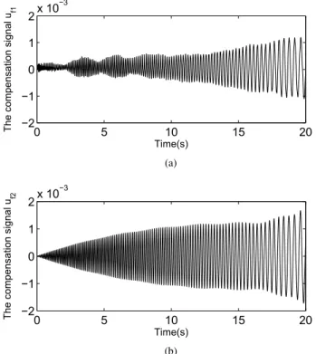
Fig. 9. Compensation signals generated by the NN compensator (Theorem 1). (a) Compensation signal for uf 1. (b) Compensation signal for uf 2.
Fig. 10. Compensation signals generated by the NN compensator (Theorem 2). (a) Compensation signal for uf 1. (b) Compensation signal for
uf 2.
two inputs plotted in Figs. 9 and 10, which shows that the mag-nitude of the compensation signals decreases with the increase of frequency, i.e., more compensation effort is emphasized in the lower frequency range. In practice, according to the frequency range of the testing signal d that we are interested
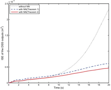
Fig. 11. Comparison of ISE plots of the DSS errors.
in, a tradeoff can be adjusted by tuning the parameters of the NN compensator.
For a clearer comparison, the integral squared errors (ISE) of the DSS controlled by LQR alone, LQR with NN compen-sator from Theorem 1, and LQR with NN compencompen-sator from Theorem 2 are shown in Fig. 11, which demonstrates that the overall performance of the case with LQR and NN com-pensators significantly outperforms the case with LQR control alone, and in particular, the NN compensator from Theorem 2 outperforms the NN compensator from Theorem 1, which clearly validates the efficacy of the new adaptive law (32).
V. CONCLUSION
We proposed a novel approach to cope with the unmodeled uncertainties and nonlinearities in the DSS control problem using an adaptive NN strategy. This approach was developed by: 1) first transforming a generalized DSS framework to a reg-ulation control framework with measured disturbance rejection and feedforward compensation and 2) incorporating an NN feedforward compensation strategy into the DSS applications as a general MIMO systems. The advantage of using this approach was that no previous knowledge of the physical substructure of a DSS was required during the NN compen-sator design. We also investigated a novel adaptive law for the NN weight updating based on an appropriate weight error information, which can lead to improved performance. The real-time applications on a mechanical test rig demonstrated the efficacy of this NN compensation technique and the novel adaptation scheme.
REFERENCES
[1] D. P. Stoten and R. A. Hyde, “Adaptive control of dynamically sub-structured systems: The single-input single-output case,” in Proc. Inst.
Mech. Eng. I, Syst. Control Eng., vol. 220, no. 2, pp. 63–79, 2006.
[2] A. R. Plummer, “Model-in-the-loop testing,” in Proc. Inst. Mech. Eng.
I, J. Syst. Control Eng., vol. 220, no. 3, pp. 183–199, 2006.
[3] P. G. Maghami and K. B. Lim, “Synthesis and control of flexible systems with component-level uncertainties,” J. Dyn. Syst., Meas., Control, vol. 131, no. 5, pp. 1–9, 2009.
[4] S.-K. Lee, E. C. Park, K.-W. Min, and J.-H. Park, “Real-time substruc-turing technique for the shaking table test of upper substructures,” Eng.
Struct., vol. 29, no. 9, pp. 2219–2232, 2007.
[5] C.-P. Lamarche, R. Tremblay, P. Léger, M. Leclerc, and O. S. Bursi, “Comparison between real-time dynamic substructuring and shake table testing techniques for nonlinear seismic applications,” Earthquake Eng.
Struct. Dyn., vol. 39, no. 12, pp. 1299–1320, 2010.
[6] O. S. Bursi, C. Jia, L. Vulcan, S. A. Neild, and D. J. Wagg, “Rosenbrock-based algorithms and subcycling strategies for real-time nonlinear sub-structure testing,” Earthquake Eng. Struct. Dyn., vol. 40, no. 1, pp. 1–19, 2011.
[7] D. P. Stoten, J. Tu, G. Li, and K. Koganezawa, “Robotic subsystem testing using an adaptively controlled dynamically substructured frame-work,” in Proc. 9th IFAC Symp. Robot Control, Gifu, Japan, 2009, pp. 98–103.
[8] M. S. Williams and A. Blakeborough, “Laboratory testing of structures under dynamic loads: An introductory review,” Phil. Trans. R. Soc.
London A, vol. 359, pp. 1651–1669, Sep. 2001.
[9] M. MacDiarmid, R. Daniel, and M. Bacic, “A novel controller design methodology for uncertain non-linear hardware-in-the-loop simulators,” in Proc. 46th IEEE Conf. Decision Control, 2007, pp. 3478–3483. [10] D. P. Stoten, J. Tu, and G. Li, “Adaptive control of generalised
dynamically substructured systems,” in Proc. 17th IFAC World Congr., Seoul, Korea, 2008, pp. 14090–14095.
[11] D. P. Stoten, J. Tu, and G. Li, “Synthesis and control of generalised dynamically substructured systems,” in Proc. Inst. Mech. Eng. I, Syst.
Control Eng., vol. 223, no. 3, pp. 371–392, 2009.
[12] D. J. Wagg and D. P. Stoten, “Substructuring of dynamical systems via the adaptive minimal control synthesis algorithm,” Earthquake Eng.
Stuct. Dyn., vol. 30, no. 6, pp. 865–877, 2001.
[13] S. A. Neild, D. P. Stoten, D. Drury, and D. J. Wagg, “Control issues relating to real-time substructuring experiments using a shaking table,” Earthquake Eng. Struct. Dyn., vol. 34, no. 9, pp. 1171–1192, 2005.
[14] A. P. Darby, M. S. Williams, and A. Blakeborough, “Stability and delay compensation for real-time substructure testing,” J. Eng. Mech., vol. 128, no. 12, pp. 1276–1284, 2002.
[15] G. Li, D. P. Stoten, and J. Tu, “Model predictive control of dynamically substructured systems with application to a servohydraulically actuated mechanical plant,” IET Control Theory Appl., vol. 4, no. 2, pp. 253–264, 2010.
[16] G. Li, G. Herrmann, D. P. Stoten, J. Tu, and M. C. Turner, “Application of a novel robust anti-windup technique to dynamically substructured systems,” in Proc. Amer. Control Conf., Baltimore, MD, USA, 2010, pp. 6757–6762.
[17] G. Li, G. Herrmann, D. P. Stoten, J. Tu, and M. C. Turner, “A novel robust disturbance rejection anti-windup framework,” Int. J. Control, vol. 84, no. 1, pp. 123–137, 2011.
[18] G. Li, G. Herrmann, D. P. Stoten, J. Tu, and M. C. Turner, “Appli-cation of robust antiwindup techniques to dynamically substructured systems,” IEEE/ASME Trans. Mech., vol. 18, no. 1, pp. 263–272, Feb. 2013.
[19] J. Na, G. Herrmann, X. Ren, and P. Barber, “Adaptive discrete neural observer design for nonlinear systems with unknown time delay,” Int. J. Robust Nonlinear Control, vol. 21, no. 6, pp. 625–647, 2011.
[20] F. L. Lewis, S. Jagannathan, and A. Yesildirek, Neural Network Control
of Robot Manipulators and Nonlinear Systems. Philadelphia, PA, USA:
Taylor & Francis, 1999.
[21] S. S. Ge, C. C. Hang, and T. H. Lee, Stable Adaptive Neural Network
Control. Boston, MA, USA: Kluwer, 2002.
[22] M. M. Polycarpou, “Stable adaptive neural control scheme for nonlinear systems,” IEEE Trans. Autom. Control, vol. 41, no. 3, pp. 447–451, Mar. 1996.
[23] F. C. Chen and C. C. Liu, “Adaptively controlling nonlinear continuous-time systems using multilayer neural networks,” IEEE Trans. Autom.
Control, vol. 39, no. 6, pp. 1306–1310, Jun. 1994.
[24] P. P. San, B. Ren, S. S. Ge, T. H. Lee, and J. Liu, “Adaptive neural network control of hard disk drives with hysteresis friction nonlinearity,”
IEEE Trans. Control Syst. Technol., vol. 19, no. 2, pp. 351–358,
Mar. 2011.
[25] J. Na, X. Ren, G. Herrmann, and Z. Qiao, “Adaptive neural dynamic surface control for servo systems with unknown dead-zone,” Control
Eng. Pract., vol. 19, no. 11, pp. 1328–1343, 2011.
[26] C. L. Lin and Y. H. Hsiao, “Adaptive feedforward control for disturbance torque rejection in seeker stabilizing loop,” IEEE Trans. Control Syst.
Technol., vol. 9, no. 1, pp. 108–121, Jan. 2001.
[27] D. Gorinevsky and L. Feldkamp, “RBF network feedforward compensa-tion of load disturbance in idle speed control,” IEEE Control Syst. Mag., vol. 16, no. 6, pp. 18–27, Dec. 1996.
[28] X. Ren, C. Lai, V. Venkataramanan, F. Lewis, S. Ge, and T. Liew, “Feedforward control based on neural networks for disturbance rejec-tion in hard disk drives,” IET Control Theory Appl., vol. 3, no. 4, pp. 411–418, Apr. 2009.
[29] X. Ren, F. L. Lewis, and J. Zhang, “Neural network compensation control for mechanical systems with disturbances,” Automatica, vol. 45, no. 5, pp. 1221–1226, 2009.
[30] J. Na, G. Herrmann, X. Ren, M. Mahyuddin, and P. Barber, “Robust adaptive finite-time parameter estimation and control of nonlinear sys-tems,” in Proc. IEEE Multi-Conf. Syst. Control ISIC, Denver, CO, USA, Sep. 2011, pp. 1014–1019.
[31] G. Li, J. Na, D. Stoten, and X. Ren, “Adaptive feedforward control for dynamically substructured systems based on neural network compensa-tion,” in Proc. IFAC World Congr., Milano, Italy, 2011, pp. 944–949. [32] B. L. Walcott and S. H. Zak, “Combined observer-controller synthesis
for uncertain dynamical systems with applications,” IEEE Trans. Autom.
Control, vol. 18, no. 1, pp. 88–104, Jan./Feb. 1988.
[33] H. Kwakernaak and R. Sivan, Linear Optimal Control Systems. New York, NY, USA: Wiley, 1972.
Guang Li (M’09) received the B.E. degree in
indus-trial automation and the M.E. degree in control the-ory and control engineering from the University of Science and Technology, Beijing, China, in 2000 and 2003, respectively, and the Ph.D. degree from the Control Systems Centre, University of Manchester, Manchester, U.K., in 2007.
He has been a Post-Doctoral Researcher with the University of Bristol, Bristol, U.K., University of Exeter, Exeter, U.K., since 2007. He is currently with Pennsylvania State University, University Park, PA, USA. His current research interests include control systems and applications, including hybrid dynamic system testing, wave energy, and battery systems.
Jing Na received the B.S. and Ph.D. degrees from
the School of Automation, Beijing Institute of Tech-nology, Beijing, China, in 2004 and 2010, respec-tively.
He was a Visiting Student with the Technical University of Catalonia, Barcelona, Spain, in 2008. From 2008 to 2009, he was a Research Collaborator with the Department of Mechanical Engineering, University of Bristol, Bristol, U.K. Since 2010, he has been with the Faculty of Mechanical and Elec-trical Engineering, Kunming University of Science and Technology, Kunming, China. His current research interests include adaptive control, neural networks, parameter estimation, repetitive control, and nonlinear control and applications. He was a Post-Doctoral Fellow with ITER Organization, Cadarache, France, from 2011 to 2012.
David P. Stoten received the Degree (Hons.) in
mechanical engineering from the University of Sal-ford, SalSal-ford, U.K., in 1974, the Ph.D. degree from Trinity College, University of Cambridge, Cam-bridge, U.K., and the D.Eng degree in Dynamics and Control from the University of Bristol, Bristol, U.K., in 1993.
He was a Research Engineer on missile flight con-trol systems with the British Aircraft Corporation, London, U.K. He was a Research Fellow with Girton College, Cambridge, in 1979. From 1979 to 1983, he was a Lecturer of mechanical engineering with the University of Liverpool, Liverpool, U.K. In 1983, he became a Lecturer and Reader with the University of Bristol, Bristol, U.K. He was a Professor of control and dynamics in 1994. From 1998 to 2004, he was the Head of Department of Mechanical Engineering, University of Bristol. His current research interests include adaptive control, multivariable control, nonlinear control, and the control of dynamically substructured (hybrid) systems.
Dr. Stoten is a fellow of the Institution of Mechanical Engineers.
Xuemei Ren received the B.S. degree from
Shan-dong University, ShanShan-dong, China, in 1989, and the M.S. and Ph.D. degrees in control engineering from the Beijing University of Aeronautics and Astronau-tics, Beijing, China, in 1992 and 1995, respectively.
She is currently a Professor with the School of Automation, Beijing Institute of Technology, Bei-jing. Her current research interests include intelli-gent systems, neural networks, adaptive control, and servo systems.
![Fig. 1. Linear control DSS framework of [1].](https://thumb-us.123doks.com/thumbv2/123dok_us/805899.2601873/3.918.494.819.75.345/fig-linear-control-dss-framework-of.webp)