Space Vector Taylor-Fourier Models for
Synchrophasor, Frequency and ROCOF
Measurements in Three-Phase Systems
Paolo Castello,
Member, IEEE,
Roberto Ferrero,
Senior Member, IEEE,
Paolo Attilio Pegoraro,
Member, IEEE,
Sergio Toscani,
Member, IEEE
Abstract—Taylor-Fourier (TF) filters represent a powerful tool to design PMU algorithms able to estimate synchrophasor, frequency and rate of change of frequency (ROCOF). The resulting techniques are based on dynamic representations of the synchrophasor, hence they are particularly suitable to track the evolution of its parameters during time-varying conditions. Electrical quantities in power systems are typically three-phase and weakly unbalanced, but most PMU measurement techniques are developed by considering them as a set of three single-phase signals; on the contrary, this peculiarity can be favorably exploited to improve accuracy and reduce the computational cost. In this respect, the present paper proposes to directly perform the TF expansion of the space vector (SV) samples obtained from three-phase measurements. A new paradigm allows to indepen-dently estimate positive and negative sequence synchrophasors along with system frequency and ROCOF, leveraging the three-phase characteristics. Performance of the proposed technique is assessed by using test signals inspired by standard IEEE C37.118.1-2011, including noise as well as magnitude and phase unbalance. Achieved results highlight the flexibility of the en-hanced SV-based approach, which is capable to combine excellent dynamic performance together with accurate estimation of both positive and negative sequence components.
Index Terms—Phasor Measurement Unit (PMU), Synchropha-sor estimation, Frequency, Rate of Change of Frequency (RO-COF), Voltage Measurement.
I. INTRODUCTION
Phasor Measurement Units (PMUs) are synchronized de-vices intended to measure amplitude, phase angle, frequency and rate of change of frequency (ROCOF) of electrical sig-nals in power networks. Initially designed for transmission networks [1], they are expected to become a widespread tool also in electric distribution systems, being considered as promising to pave the implementation of smart grids [2] able to automatically control the network operation based on an accurate, fast and reliable monitoring.
PMUs label data with time-tags referred to a common timescale (the coordinated universal time, UTC, obtained from a GPS receiver is typically adopted), so that measurements
P. Castello and P. A. Pegoraro are with the Department of Electrical and Electronic Engineering, University of Cagliari, 09123 Cagliari, Italy (e-mail: [email protected]; [email protected])
R. Ferrero is with the Department of Electrical Engineering and Electronics, University of Liverpool, Liverpool L69 3GJ, U.K. (e-mail: [email protected]).
S. Toscani is with the Dipartimento di Elettronica, Informazione e Bioingegneria, Politecnico di Milano, 20133 Milan, Italy (e-mail: [email protected]).
collected on a wide area can be correlated and employed even in real-time, thus enabling an accurate representation of the operating conditions that can be exploited in grid control applications [2].
PMU algorithms are designed to extract the fundamental frequency component, along with the corresponding frequency and ROCOF, coping with different conditions that may occur in electrical signals: dynamics, harmonic and interharmonic disturbances, rapid variations, etc.
Several algorithms have been proposed in recent literature (see [2] for a review), based on a wide range of estimation techniques and tailored according to specific test conditions. Signal dynamics is particularly important, since PMUs are designed to operate even at high reporting rates (50 frames/s or even higher in 50 Hz systems) in order to track amplitude, phase angle and frequency changes. The last standard for synchrophasor measurements IEEE C37.118.1-2011 [3] (along with its amendment [4]) introduces the concept of dynamic synchrophasor and prescribes specific tests that can be repre-sentative of both slow variations, like amplitude or phase angle modulations and linear frequency ramps, and abrupt changes, such as amplitude and phase angle steps. Limits in terms of accuracy or dynamic response are reported for the different test conditions.
An interesting approach to measure dynamic signal pa-rameters was proposed in [5] where a Taylor expansion of the phasor around the measurement instant is adopted to better describe its time evolution (Taylor-Fourier approach, TF), thus allowing a more accurate dynamic tracking of the related quantities. Such model has been exploited by different algorithms. In [6], [7], for instance, estimations are based on the discrete Fourier transform (DFT) and the model is employed to correct them by considering the effects due to parameter variations. In [8] the Taylor expansion approach is used to extend the interpolated DFT algorithm, while in [9] a two-channel PMU algorithm based on a Taylor approach is employed to achieve simultaneous compliance with P and M classes requirements defined by [3], [4].
All the above algorithms are designed starting from a single-phase signal. Recently, the idea of exploiting the typical characteristics of three-phase quantities to define PMU algo-rithms has been proposed. In particular, in [10] a space vector (SV) based algorithm is introduced. The positive sequence synchrophasor is obtained from the SV by means of an IIR filtering stage and two least-squares FIR interpolators: a first
one for amplitude estimation and a second one allowing phase angle and frequency measurements. In [11], all the quantities are derived by FIR filtering the real and imaginary parts of the SV. In particular, frequency and ROCOF are obtained by applying properly-designed first and second order partial-band FIR differentiators, respectively, which allow designing algo-rithms that are compliant with the performance classes defined in [3] and [4]. In [12], the SV transformation is considered as a preliminary stage for the Interpolated DFT computation, thus allowing better estimations under off-nominal frequency conditions.
Other works exploiting similar approaches can be found in the literature. As an example, [13] and [14] use the SV transformation on a stationary reference frame in order to estimate the positive sequence phasor. On the contrary, [15] measure the positive sequence synchrophasor with respect to a rotating reference frame, which provides three-phase demodulation.
In [16] conventional TF filtering and the SV approach are combined in order to permit the estimation of positive and negative sequence synchrophasors, frequency and ROCOF that characterize three-phase signals with considerable reduction in terms of computational burden.
It should be noticed that positive and negative sequence components have very different magnitudes during typical operation; a first consequence is that the challenge to be faced when they have to be extracted from the complex SV signal are extremely different in the two cases. On the one hand negative component measurement may suffer from severe spectral interference due to the positive sequence term acting as a very large disturbance that have to be suppressed with strong filtering. On the other hand, dynamic performance is much more important as far as the positive sequence synchrophasor estimate. Furthermore, since the spectrum of the SV signal is far from being hermitian, there is no reason to design TF filters having the same expansion order for the positive and negative sequence terms.
Starting from the previous considerations, this paper pro-poses a radically new approach using completely different TF filters for positive and negative sequence estimations; in turns, these filter may be characterized by different expansion orders for the positive and negative sequence components. The additional degrees of freedom in filter design allow a more effective exploitation of the three-phase peculiarities of electrical signals. For example, the proposed technique allows to finely tune the filters to achieve an accurate and prompt detection of unbalance [17], which is key to avoid severe contingencies and blackouts [18].
The proposed approach is validated and discussed by means of simulations intended to show the impact of the TF filter design parameters on the overall measurement accuracy. This allows highlighting the advantages and the generality of the proposed framework for PMU algorithm design.
II. TAYLOR-FOURIERAPPROACH INTHREE-PHASE
SYSTEMS
A. Conventional Taylor-Fourier Synchrophasor Estimation As stated in the introduction, dynamic phasor measure-ments through Taylor-Fourier filtering were proposed in [5] to accurately track slow transients of electrical signals in ac power system applications. In several works, this ap-proach has been exploited to design PMU algorithms having remarkable dynamic performance. The first step is writing the synchrophasor model: supposing operation near the rated frequencyf0(corresponding to the angular frequencyω0), the
time evolutions of its real and imaginary parts are slow in the common, UTC-synchronized reference frame rotating at the angular speedω0. Therefore they can be represented with
truncated Taylor expansions (up to theKth order) around the generic measurement instanttr:
¯ x(t−tr)' K X k=0 ¯ X(k)(tr) (t−tr)k k! (1)
wherex¯(t−tr)is the dynamic synchrophasor whileX¯(k)(tr)
represents itskth derivative in the measurement instant. The previous expression can be rewritten by using the vector notation. To this purpose, let us introduce the complex column vectorp¯K(tr)of the phasor derivatives and the real row vector
a: ¯ pK(tr) = ¯ X(0)(tr) X¯(1)(tr) · · · X¯(K)(tr) T (2) a(t−tr) = h 1 t−tr · · · (t−tr) K K! i (3) whereTdenotes the transpose operator.
Therefore:
¯
x(t−tr)'a(t−tr)¯pK(tr) (4)
The time domain expression of the signal can be obtained by projecting its synchrophasor on the real axis of a stationary reference frame, as we do when the inverse Steinmetz trans-form is applied to a phasor:
x(t−tr)'
√
2<ha(t−tr)¯pK(tr)ejω0(t−tr)
i (5) denoting with ∗ the complex conjugate operator, (5) can be rewritten in a more convenient form1:
x(t−tr) = = a(t−tr)ejω0(t−tr) a(t−tr)e−jω0(t−tr) p¯(tr) √ 2 (6)
wherep¯(tr)is defined as: ¯ p(tr) = ¯ pK(tr) ¯ p∗K(tr) (7) It is evident that, in general, the time domain expression is a non-holomorphic function of the K+ 1 synchrophasor derivatives in the measurement instant tr, since it involves 1The equality symbol is used instead of similarity symbol from here on for the sake of simplicity, thus assuming that the model holds true.
also their complex conjugates. Estimating the synchrophasor means inverting (6), but it is an underdetermined problem: at least 2K+ 2independent constraints are required. To this purpose, let us suppose to have available aN-sample window (N odd and greater than2K+2) of the time domain waveform centered intr. Assuming that such samples are collected with
a uniform interval Ts, low enough to avoid aliasing artifacts,
they can be arranged in a column vector x(tr):
x(tr) = x(tr+N2−1)Ts .. . x(tr−N2−1)Ts (8)
and the following system of equations can be set up:
x(tr) = 1 √ 2 ¯ ΦA Φ¯∗Ap¯(tr) = 1 √ 2 ¯ Bp¯(tr) (9) where: A= a(N−21Ts) .. . a(−N−1 2 Ts) (10) ¯ Φ= ejω0N−21Ts . .. 1 . .. e−jω0N−21Ts (11)
The synchrophasor and its derivatives can be obtained by minimizing the norm of the error between model output and waveform samples. It requires computing the matrixH¯ as the pseudoinverse of B¯: ˆ ¯ p(tr) = √ 2( ¯BHB¯)−1B¯Hx(tr) = √ 2 ¯Hx(tr) (12)
where H denotes the Hermitian transpose operator whileˆ
indicates that the quantity is an estimate. From (12) it can be noticed that, with this approach, measuring the synchrophasor and its derivatives is a linear operation, corresponding to apply a bank of FIR filters of length N (the rows of matrix √
2 ¯H, two for each derivative order including the zeroth) to the time-domain signal. The order K of the expansion and the window length N are the design parameters that allow tailoring their frequency response functions in order to match specific requirements. In turn, frequency and ROCOF estimates are provided by the following formulas, that require at first and second order expansions, respectively:
ˆ f(tr) =f0+ 1 2π =hXˆ¯p(1)(tr)·Xˆ¯ (0)∗ p (tr) i ˆ ¯ Xp(0)(tr) 2 \ ROCOF(tr) = 1 π =hXˆ¯p(2)(tr) ¯X (0)∗ p (tr) i 2 ˆ ¯ Xp(0)(tr) 2 + − <hXˆ¯p(1)(tr) ˆX¯ (0)∗ p (tr) i =hXˆ¯p(1)(tr) ˆX¯ (0)∗ p (tr) i ˆ ¯ Xp(0)(tr) 4 (13)
A closer look at (12) allows several, interesting consider-ations. Reminding (7), it returns not only the synchrophasor derivatives (firstK+ 1rows ofpˆ¯(tr)), but also their complex
conjugates (last K + 1 rows of pˆ¯(tr)), which is redundant
information. Another closely related issue is that the estimates of the synchrophasor and its derivatives are affected by in-terference due to the dynamic image component when the synchrophasor model is not exact.
B. Straightforward Extension to Three-phase Systems For both economic and technical reasons, ac power systems are inherently three-phase. For a given electrical quantity, the Taylor-Fourier estimator (12) can be straightforwardly applied to each of the three phases; adopting a matrix formulation is more convenient. To the purpose, let us define the matrixes
Xabc(tr) and P¯abc(tr) containing the samples and the
syn-crophasor derivatives of the three phases, respectively:
XTabc(tr) = xT a(tr) xT b(tr) xT c(tr) P¯ T abc(tr) = ¯ pT a(tr) ¯ pT b(tr) ¯ pT c(tr) (14)
where the subscripta,b orcindentifies a particular phase. In this way, the three-phase model can be easily written:
XTabc(tr) = 1 √ 2 ¯ PTabc(tr) ¯BT (15)
and it can be inverted in a least squares (LS) sense to obtain the estimates of the synchrophasor, their derivatives and their conjugates: ˆ ¯ PTabc(tr) = √ 2XTabc(tr) ¯HT (16)
This formulation maintains all the drawbacks of the single-phase implementation. Furthermore, different frequency and ROCOF estimations can be performed by applying (13) to each of the three phases (see also [16]. However, a unique frequency and ROCOF has to be provided for a three-phase quantity. A straightforward yet inefficient possibility is computing the mean of the three single-phase estimates.
C. Symmetrical Components and Taylor-Fourier Filters The analysis of three-phase systems is much more effective when carried out by using the symmetrical components. To this purpose, let us define the transformation matrix S¯ that allows obtaining the symmetrical components from the three phasors (α¯,ej2π/3): ¯ S= √1 3 1 α¯ α¯2 1 α¯2 α¯ 1 1 1 (17)
With this formulation S¯ is unitary, hence its inverse corre-sponds to the Hermitian transposeS¯H. The symmetrical
com-ponents transformation can be applied to the matrixPˆ¯T
abc(tr): ˆ ¯ PTS(tr) = ¯SP¯Tabc(tr) = √ 2¯SXTabc(tr) ¯HT (18)
and, by performing simple considerations, it can be noticed that the resulting matrixPˆ¯T
S(tr)shows the following structure:
ˆ ¯ PTS(tr) = ˆ ¯ pT +(tr) pˆ¯∗−T(tr) ˆ ¯ pT −(tr) pˆ¯∗+T(tr) ˆ ¯ pT 0(tr) pˆ¯∗0T(tr) (19)
where pˆ¯s(tr) with s ∈ {+,−,0} is the column vector
containing the estimates of the positive, negative or zero sequence synchrophasors together with the corresponding K
derivatives. Hence, adopting the usual notation:
ˆ ¯ ps(tr) = h ˆ ¯ Xs(0)(tr) Xˆ¯ (1) s (tr) · · · Xˆ¯ (K) s (tr) iT (20) where Xˆ¯s(k)(tr)is the generic sequencepsynchrophasor kth
derivative.
Looking at (19) it becomes evident that the first two rows of pˆ¯s(tr)carry the same information. In particular, when the
zero sequence component isa priorinegligible or not present (e.g. line voltages), the first row synthesize all the parameters describing the dynamic phasors of the three-phase quantity. Using (17), (18), (19) it can be written:
ˆ ¯ pT+(tr) p¯ˆ∗−T(tr) = r 2 3 1 α¯ α¯2 XTabc(tr) ¯HT (21) In (21) theN samples of the SV related to the three phase quantity can be recognized. Defining:
ˆ ¯ pSV(tr) = ˆ ¯ p+(tr) ˆ ¯ p∗−(tr) (22) ¯ xTSV(tr) = r 2 3 1 α¯ α¯2 XTabc(tr) (23)
therefore (21) can be expressed as:
ˆ ¯
pSV(tr) = ¯H¯xSV(tr) (24)
The previous equation applies the Taylor-Fourier expansion to the SV signal, performed by inverting the following expres-sion in the LS sense:
¯
xSV(tr) = ¯Bp¯SV(tr) (25)
This approach features many advantages with respect to separately processing the phase signals as in the previous subsection. First of all, no redundant data is returned by (24), since, when looking at the SV, it is a linear, holomorphic function of the positive and the conjugate of the negative sequence synchrophasors. Several applications only require to measure the positive sequence synchrophasor: in this way it is directly obtained with clear advantages in terms of computational cost, since three single-phase estimations are avoided. Furthermore, frequency and ROCOF of a three-phase quantity are typically obtained starting from the time evolution of the phase angle of the fundamental, positive sequence synchrophasor. In fact, the reference P and M class methods proposed by [3], [4] adopt this definition. Finally, it should be noticed that the positive sequence synchrophasor carries most of the information about the three-phase quantity because of the typically weak unbalance levels in power systems. Therefore, supposing that the phase signals are purely sinusoidal, the estimate of the positive sequence synchrophasor is only affected by interference with the negative sequence component, which is surely much lower in amplitude. In this respect, a single-phase estimation is much more critical, since it may suffer from interaction with the large image component. D. Taylor Fourier Filters of the Space Vector
In the previous paragraph, it has been shown how the positive and negative sequence synchrophasors (and their derivatives) can be estimated by applying aKth order Taylor-Fourier filter bank to the SV samples. The results are the same as those obtained by performing three Taylor-Fourier transforms of the single-phase signals (with the same order
K) and then computing the symmetrical components thanks to the Fortescue transformation; however, the computational burden is considerably reduced. On the other hand, starting from single-phase quantities implies that the expansion orders of the positive and negative sequence synchrophasors must be the same. This constraint can be removed by thinking in terms of SV signal while reminding the relationship with positive and negative sequence dynamic synchrophasors, modeled withK+
andK−expansion orders respectively. Therefore, let us define:
¯ ps(tr) = h ¯ Xs(0)(tr) X¯ (1) s (tr) · · · X¯ (Ks) s (tr) iT (26) as(t−tr) = h 1 t−tr · · · (t−tr)Ks Ks! i (27) withs∈ {+,−}. Using the relationship between symmetrical components synchrophasors and SV, the model results:
¯ xSV(t−tr) =a+(t−tr)¯p+(tr)ejω0(t−tr)+ +a−(t−tr)¯p∗−(tr)e−jω0(t−tr)= = a+(t−tr)ejω0(t−tr) a−(t−tr)e−jω0(t−tr) ¯ pSV(tr) (28) where the last term is obtained introducing p¯SV(tr) ,
¯ pT
+(tr) p¯H−(tr)
T
and definingx¯SV(tr)(N sample
win-dow of the SV signal centered in tr) as in (22) and (23): ¯
xSV(tr) =
¯
where: As= as(N2−1Ts) .. . as(−N2−1Ts) (30)
with s ∈ {+,−}. Assuming that the usual hypothesis are met and that N ≥ K+ +K− + 2, the previous problem is
overderdetermined and B¯± has a left pseudoinverse H¯± so
that (29) can be solved in the least squares sense as follows:
¯ pSV(tr) = ¯H±x¯SV(tr) = B¯H±B¯± −1 ¯ xSV(tr) (31) ¯
H± contains the bank of FIR filters that allows obtaining
ˆ ¯
pSV (namely the estimate of p¯SV) for each window of
SV samples, being (24) formally identycal to (31). The first
K++ 1rows of H¯± allow computing the positive sequence
synchrophasor (and its derivatives) while the last K− + 1
rows permit evaluating the conjugate of the negative sequence synchrophasor (together with its derivatives).
Now, it should be noticed that the challenges to be faced when the positive or negative sequence synchrophasor have to be measured are very different. For example, the signal to noise ratio and the spectral interference may heavily affect the estimation of the negative sequence component, while their impact is not so pronounced as for the positive sequence synchrophasor measurement. On the one hand, if frequency and ROCOF have to be measured, at least a second order expansion of the positive sequence synchrophasor is required; on the other hand this is not mandatory as far as the neg-ative sequence synchrophasor. Furthermore, good dynamic performance is needed to follow the evolution of the positive sequence synchrophasor, while usually it does not apply to the negative sequence synchrophasor. It should be noticed that generally increasing the order of the expansion allows better dynamic performance (flatter bandpass) but at the expense of lower frequency selectivity, which makes the estimate more sensitive to spectral interference and broadband noise.
Therefore, an interesting solution that allows a more flex-ible tuning of the algorithm is to employ different models (thus different Taylor Fourier expansion orders) for estimating the positive and the negative synchrophasor. Thanks to the proposed approach, it is possible to choose a couple of expansion orders K++ andK+− that will be used to obtain
the filters for estimating the positive sequence synchrophasor and its two first derivatives (first three rows of the resulting pseudoinverse H+). At the same time, a potentially different
couple of expansion ordersK−+ andK−− can be employed
to compute the filters for estimating the (conjugate of the) negative sequence synchrophasor (namely the first row of the pseudoinverseH−).
III. TESTS ANDRESULTS
Hybrid SV-TF algorithms proposed in Section II-D have been tested and compared by means of numerical simu-lations under Matlab environment. A sampling frequency
fs = 10 kHz is adopted and a 50-Hz system is considered
(f0 = 50 Hz). Synchronization error is neglected since
it would affect every algorithm in the same way, namely
producing a phase-angle error due to the clock offset (typical GPS time error is<100ns and timebase error<1µs).
Different TF filters can be defined according to the selected expansion orders (namely K++ and K+− when focusing on
the positive-sequence estimation) and window length. In the following, the smallest odd number of samples including an integer number of nominal cycles is used.
Synchrophasor, frequency and ROCOF are evaluated sample-by-sample as if a reporting rate equal to fs were
considered. The performance of the algorithms is quantified and expressed in terms of total vector error (TVE)%, absolute frequency error (FE) and absolute ROCOF error (RFE) for synchrophasor, frequency and ROCOF estimations, respec-tively, as defined by [3].
Algorithms are tested with different input signals, covering both steady-state and dynamic conditions; maximum TVE, FE and RFE are computed in each test. Since the aim is assessing algorithm performance and highlighting the impact of design parameters, the test signals are only inspired by those of the compliance tests in IEEE C37.118.1 (and IEEE C37.118.1a) [3], [4], without in any way claiming to be exhaustive with respect to P or M class requirements. While in [16] the focus was about the advantages of a three-phase TF implementation, in this paper the generalization of the model allowed by the SV approach is considered in order to show how the addi-tional degrees of freedom can be exploited. According to this purpose, it is more useful to test the algorithm performance under specific yet realistic conditions, thus including also the presence of noise and unbalance which are typically neglected by the relevant standards.
Firstly, following the achievements of Section II, a dy-namic test is performed. Three-phase, amplitude modulated signals are applied; sinusoidal modulation having frequency
fm∈[0,5]Hz (with a step of0.1Hz) is adopted. The generic
expression of the test signal is given by:
xabc(t) = √ 2X(1 +xm(t))· < ej2πf0t 1 α¯2 α¯ T (32) wherexabc(t)is the vector of phase signals,X is the common
rms magnitude and:
xm(t) =kxcos (2πfmt) (33) kx represents the amplitude modulation depth; the highest
value considered by [4] has been adopted, thuskx= 0.1.
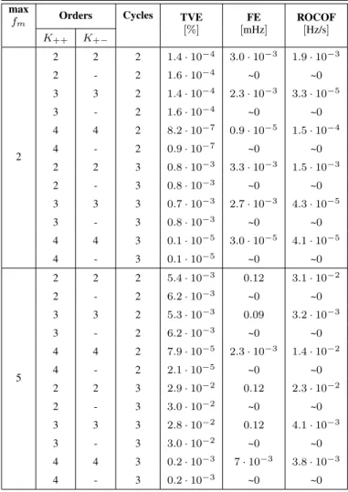
Table I shows the maximum TVE (for positive sequence synchrophasor estimation), FE and RFE values for two mod-ulation frequency ranges ([0,2]Hz and[0,5]Hz, respectively) when the algorithm is implemented with different positive sequence expansion orders; window lengths corresponding to 2 or 3 nominal cycles are used. The negative sequence component is either expanded to the same order as the positive one (K+−=K++) or excluded from the model. All the errors
are low and only slight advantages are obtained by increasing
K++. It is interesting to notice that considering the negative
sequence component does not give significant improvements. This perfectly reflects the considerations performed in Section II, since when a balanced three-phase input is acquired, no
negative sequence component is present and thus, a single-sideband SV signal model holds. The slight improvement achieved by including also the negative sequence contribution is due to undermodeling: the model error due to the truncated TF expansion is partially embedded by the negative sequence term.
TABLE I
MAXIMUMTVE, FE, RFEUNDER AMPLITUDE MODULATION
max
fm Orders Cycles TVE [%] FE [mHz] ROCOF [Hz/s] K++ K+− 2 2 2 2 1.4·10−4 3.0·10−3 1.9·10−3 2 - 2 1.6·10−4 ~0 ~0 3 3 2 1.4·10−4 2.3·10−3 3.3·10−5 3 - 2 1.6·10−4 ~0 ~0 4 4 2 8.2·10−7 0.9·10−5 1.5·10−4 4 - 2 0.9·10−7 ~0 ~0 2 2 3 0.8·10−3 3.3·10−3 1.5·10−3 2 - 3 0.8·10−3 ~0 ~0 3 3 3 0.7·10−3 2.7·10−3 4.3·10−5 3 - 3 0.8·10−3 ~0 ~0 4 4 3 0.1·10−5 3.0·10−5 4.1·10−5 4 - 3 0.1·10−5 ~0 ~0 5 2 2 2 5.4·10−3 0.12 3.1·10−2 2 - 2 6.2·10−3 ~0 ~0 3 3 2 5.3·10−3 0.09 3.2·10−3 3 - 2 6.2·10−3 ~0 ~0 4 4 2 7.9·10−5 2.3·10−3 1.4·10−2 4 - 2 2.1·10−5 ~0 ~0 2 2 3 2.9·10−2 0.12 2.3·10−2 2 - 3 3.0·10−2 ~0 ~0 3 3 3 2.8·10−2 0.12 4.1·10−3 3 - 3 3.0·10−2 ~0 ~0 4 4 3 0.2·10−3 7·10−3 3.8·10−3 4 - 3 0.2·10−3 ~0 ~0
Similar results can be obtained when phase angle modu-lation is considered. The modulating signal is still sinusoidal and its frequency fm in swept in the same ranges as before.
Table II shows that there are significant values only for FE and RFE, particularly when higher modulation frequencies are considered. Results reflect the above discussion, since errors are very similar notwithstanding the different models adopted. Once again, measurement improvements are linked to the order ofK++, which extends the filters bandwidths.
It should be noticed that the choice of the TF expansion orders have significant impact in the presence of broadband noise which typically affects the samples. Figs. 1 and 2 show the results when steady-state signals at the rated frequency with superimposed uniform noise are applied. The root mean square errors of frequency and ROCOF estimations (FErms
and RFErms, respectively) are reported at increasing noise
levels, with signal to noise ratios (SNRs) in the range40÷90
TABLE II
MAXIMUMTVE, FE, RFEUNDER PHASE MODULATION
max
fm Orders Cycles TVE [%] FE [mHz] ROCOF [Hz/s] K++ K+− 2 2 2 2 1.7·10−4 1.2 1.1·10−2 2 - 2 1.5·10−4 1.3 1.1·10−2 3 3 2 1.3·10−4 2.0·10−3 1.1·10−2 3 - 2 1.5·10−4 1.6·10−3 1.1·10−2 4 4 2 9.8·10−7 1.3·10−3 1.1·10−4 4 - 2 1.3·10−7 1.8·10−3 0.1·10−4 2 2 3 7.2·10−3 2.8 2.5·10−2 2 - 3 7.5·10−4 2.9 2.6·10−2 3 3 3 6.9·10−4 8.3·10−3 2.4·10−2 3 - 3 7.5·10−4 8.2·10−3 2.6·10−2 4 4 3 1.5·10−6 7.9·10−3 7.1·10−5 4 - 3 1.4·10−6 7.9·10−3 5.5·10−5 5 2 2 2 5.0·10−3 19 0.42 2 - 2 5.8·10−3 20 0.44 3 3 2 4.9·10−3 0.14 0.41 3 - 2 5.8·10−3 0.16 0.44 4 4 2 1.0·10−4 0.13 1.1·10−2 4 - 2 0.3·10−4 0.17 0.3·10−2 2 2 3 2.7·10−2 42 0.96 2 - 3 2.8·10−2 43 0.98 3 3 3 2.6·10−2 0.74 0.94 3 - 3 2.8·10−2 0.78 0.98 4 4 3 2.6·10−4 0.75 0.13 4 - 3 3.4·10−4 0.83 0.14
dB. Typical SNR values of acquired signals are between 60
and 80 dB (e.g. 72dB corresponds to 12 effective bits) but sometimes they can be even lower [19]. A wider range has been explored in order to study the behavior also in case of extremely good or very poor signal to noise ratio. FErms and
RFErms are employed since maximum errors can be highly
uncertain because of noise. The analysis is focused on a 2-cycle window andK++ values of 2 and 4 are considered.
For all the test cases, errors decrease by including only the positive sequence term in the SV model. The reduction of FErms ranges from 5.8 % for order 2 to 13.3 % for order 4,
while that of RFErmsis about6.8 %for order 2 and29.6 %for
order 4. Smaller improvements can be achieved also for TVE (up to7.1 %), but they are not reported for the sake of brevity. As expected, wideband noise rejection is strictly linked to the equivalent noise bandwidth of each filter, thus using different expansions orders for positive and negative sequence terms allows enhancing robustness with respect to noise.
All together, the reported results show that thanks to the flexibility of the proposed approach it is possible to follow the positive sequence synchrophasor, frequency and ROCOF dynamics while also guaranteeing a better immunity to dis-turbances. These considerations apply to all the tests of the
40 50 60 70 80 90
SNR [dB]
0 5 10 15FE
rms[mHz]
K ++=2 K++=K+-=2 K++=4 K ++=K+-=4Fig. 1. Impact of broadband noise: root mean square FE achieved by SV-TF with different expansion orders.
40 50 60 70 80 90
SNR [dB]
0 1 2 3 4 5 6RFE
rms[Hz/s]
K ++=2 K ++=K+-=2 K ++=4 K ++=K+-=4Fig. 2. Impact of broadband noise: root mean square RFE achieved by SV-TF with different expansion orders.
standard IEEE C37.118.1 [3], since PMU compliance tests are designed only for positive-sequence signals.
Now, it is very interesting to investigate the performance achieved with unbalanced three-phase signals which may oc-cur in real-world applications, in particular when distribution systems are considered. Tests were performed at both nominal and off-nominal frequency with different types of unbalance. Since standards [3], [4] consider only positive sequence sig-nals, these tests have been inspired by the unbalanced signals suggested in the guide IEEE C37.242 [20]. The following single-phase variations are applied:
• Magnitude variations δm: ±10 % (corresponding to
un-balance levels of 3.2 % and3.4 %)
• Phase-angle variations δφ: ±10° (corresponding to an
unbalance level of 5.8 %)
where (1 +δm) and δφ are, respectively, the amplification
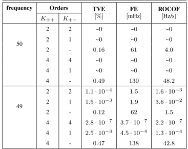
factor and the phase angle deviation applied to phase a. Table III reports the maximum TVE, FE and RFE for two frequencies and δm = +10 % when different orders are
used (2-cycle algorithms). 49 Hz and 50 Hz frequencies are
considered, as suggested by [20]. It is clear that a purely positive-sequence model K++ >0 is no longer sufficient to
match the SV and thus the errors become unacceptable. On the other end, a first order expansion (K+− = 1) is suitable
to properly consider the negative sequence component even under off-nominal frequency conditions.
TABLE III
MAXIMUMTVE, FE, RFEUNDER MAGNITUDE UNBALANCE
(δm= +10 %)
frequency Orders TVE
[%] FE [mHz] ROCOF [Hz/s] K++ K+− 50 2 2 ~0 ~0 ~0 2 1 ~0 ~0 ~0 2 - 0.16 61 4.0 4 4 ~0 ~0 ~0 4 1 ~0 ~0 ~0 4 - 0.49 130 48.2 49 2 2 1.1·10−4 1.5 1.6·10−3 2 1 1.5·10−3 1.9 3.6·10−2 2 - 0.12 62 1.5 4 4 2.8·10−7 3.7·10−7 2.2·10−7 4 1 2.5·10−3 4.5·10−4 1.3·10−4 4 - 0.47 138 42.8
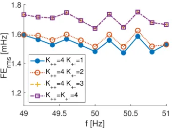
Since TF filtering is based on least squares fitting, more accurate estimations are achieved when the model is able to match the actual signal. In Figs. 3 and 4 the FErms and
RFErms results for a+10 %magnitude variation with a60dB
noise are considered in the frequency range [49,51]Hz. In particular, the errors forK++= 4 are reported with different
values of K+−. The configuration {K++, K+−} = {4,1}
gives best results for both FE and RFE with maximum error reductions with respect to the configuration {4,4} of about
12 % and29 %, respectively. It is possible to notice that the advantages with respect to the configuration {4,2} become less relevant as the frequency offset increases; the reason lies in the trade-off between stopband flatness around −f0
(that allows reucing interference with the negative sequence term) and wideband noise filtering. Similar results have been obtained for TVErms, but error reduction is lower (~7 %). Fig.
5 reports the results for a 10° variation of phase a signal (only RFErmsis reported for the sake of brevity); the previous
considerations for amplitude unbalance apply also in this case. The advantages of {4,1}are evident for frequencies close to
f0 (RFErms reduces up to 29 %); when a larger frequency
deviation occurs, the effect of the negative sequence infiltration becomes more important, hence a largerK+− (e.g.2) allows
reducing its impact.
The algorithm presented in Section II also permits to estimate the negative sequence synchrophasor. In this context the definition of the SV model becomes even more important, since, as explained in previous sections, X¯− is much lower
thanX¯+, thus resulting in a increased sensitivity to
interfer-ence with the positive sequinterfer-ence term and disturbances. Table IV shows the TVErmsvalues for the negative sequence
estima-49 49.5 50 50.5 51
f [Hz]
1.2 1.4 1.6 1.8FE
rms[mHz]
K ++=4 K+-=1 K ++=4 K+-=2 K++=4 K+-=3 K++=K+-=4Fig. 3. Root mean square FE achieved by SV-TF with different negative sequence component expansion orders under magnitude unbalance, 60dB SNR. 49 49.5 50 50.5 51
f [Hz]
0.1 0.2 0.3 0.4 0.5 0.6RFE
rms[Hz/s]
K ++=4 K+-=1 K ++=4 K+-=2 K++=4 K+-=3 K++=K+-=4Fig. 4. Root mean square RFE achieved by SV-TF with different negative sequence component expansion orders under magnitude unbalance, 60dB SNR. 49 49.5 50 50.5 51
f [Hz]
0.2 0.3 0.4 0.5 0.6RFE
rms[Hz/s]
K ++=4 K+-=1 K ++=4 K+-=2 K ++=4 K+-=3 K ++=K+-=4Fig. 5. Root mean square RFE achieved by SV-TF with different negative sequence component expansion orders under phase unbalance,60dB.
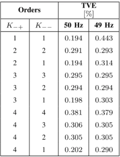
tion (2-cycle window) in the above conditions (δm= +10 %
and SNR = 60 dB) for different{K−+, K−−} couples. It is
important to notice that, as expected, TVE values are much higher than those considering positive sequence measurements. Choosing a suitable filter configuration has a dramatic impact on the accuracy: with {4,1}, for instance, it is possible to get at least a30 %error reduction at the rated frequency with respect to configurations resulting in similar TVE errors at
49Hz.
The accuracy in estimating the negative sequence syn-chrophasor have been compared to that achieved by using the well-known standard P-class method (P-C37.118.1) in [3] having the same two-cycle length. The negative sequence synchrophasor has been obtained by applying the Fortescue transformation to the estimated single-phase synchrophasors. For the above magnitude unbalance at 49Hz, with a SNR
= 60 dB, P-C37.118.1 results in RFErms ' 0.860Hz/s and
TVErms '0.383 % for the negative sequence synchrophasor,
which is much larger than almost all the configurations listed in Table IV. From another viewpoint, it is important to recall that the standard P-class method achieves maximum TVE errors which are at least two orders of magnitude larger than those reported in Tables I and II under amplitude and phase modulations.
Finally, tests have been performed also by considering signals acquired with a real data acquisition stage. Since real-world signals lack of ground-truth reference, algorithms are verified by using signals generated with an OMICRON CMC256Plus calibrator [21] synchronized with the IRIG-B output of CMIRIG-B interface [22] fed by a GPS receiver (±1µs overall synchronization accuracy). A typical PMU input level of 100 Vrms is used as reference voltage and thus a 300 Vrms NI-9225 card [23] is employed withfs= 50kHz.
As an example, the results in terms of FErms, for the +10%
magnitude unbalance and 49Hz frequency, are 0.6mHz and
1.2mHz for the configurations {K++, K+−} = {4,1} and
{4,4}, respectively. These values fully confirm the considera-tions derived from simulation results in Fig. 3. It is important to recall that the calibrator gives a stable frequency with a
0.5ppm accuracy, corresponding to less that 0.025mHz at nominal frequency.
IV. CONCLUSIONS
In this paper, a general framework to merge two powerful approaches (TF and SV) for PMU algorithm design in three-phase systems has been presented.
TF filters have been applied to estimate the positive and neg-ative sequence synchrophasors from the time domain samples obtained by applying the SV transformation. The proposed technique allows an independent estimation of the positive and negative sequences components by exploiting different Taylor expansions. This represents a very important outcome since the measurement challenges to be faced in the two cases are completely different.
Simultation results have shown that the proposed method al-lows following positive and negative sequence synchrophasors, frequency and ROCOF dynamics with remarkable accuracy
TABLE IV
ROOTMEANSQUARETVEOFX¯−ESTIMATION UNDER MAGNITUDE UNBALANCE(δm= +10 %). SNR= 60 dB Orders TVE [%] K−+ K−− 50 Hz 49 Hz 1 1 0.194 0.443 2 2 0.291 0.293 2 1 0.194 0.314 3 3 0.295 0.295 3 2 0.294 0.294 3 1 0.198 0.303 4 4 0.381 0.379 4 3 0.306 0.305 4 2 0.305 0.305 4 1 0.202 0.290
both in presence of noise and under off-nominal frequency conditions. The higher flexibility allowed by the three-phase approach permits better performance with respect to the con-ventional per-phase TF expansion.
The proposed framework is intended to permit a fine-tuning of PMU design that allows a better exploitation of the peculiarities of three-phase signals, which is extremely promising for many important applications requiring accurate estimates of the symmetrical components.
ACKNOWLEDGMENTS
Dr. Pegoraro’s work was partially funded by Fondazione di Sardegna for the research project “SUM2GRIDS, Solutions by mUltidisciplinary approach for intelligent Monitoring and Management of power distribution GRIDS”.
REFERENCES
[1] A. G. Phadke and J. S. Thorp,Synchronized Phasor Measurements and Their Applications. Springer Science, 2008.
[2] AA. VV.,Phasor Measurement Units and Wide Area Monitoring Sys-tems, 1st ed., A. Monti, C. Muscas, and F. Ponci, Eds. Academic Press, 2016.
[3] IEEE Standard for Synchrophasor Measurements for Power Systems, IEEE IEEE Std C37.118.1-2011 (Revision of IEEE Std C37.118-2005), Dec. 2011.
[4] IEEE Standard for Synchrophasor Measurements for Power Systems – Amendment 1: Modification of Selected Performance Requirements, IEEE IEEE Std C37.118.1a-2014 (Amendment to IEEE Std C37.118.1-2011), Apr. 2014.
[5] J. A. de la O Serna, “Dynamic phasor estimates for power system oscillations,”IEEE Trans. Instrum. Meas., vol. 56, no. 5, pp. 1648–1657, Oct. 2007.
[6] W. Premerlani, B. Kasztenny, and M. Adamiak, “Development and implementation of a synchrophasor estimator capable of measurements under dynamic conditions,”IEEE Trans. Power Del., vol. 23, no. 1, pp. 109–123, Jan. 2008.
[7] R. K. Mai, Z. Y. He, L. Fu, B. Kirby, and Z. Q. Bo, “A dynamic synchrophasor estimation algorithm for online application,”IEEE Trans. Power Del., vol. 25, no. 2, pp. 570–578, Apr. 2010.
[8] D. Petri, D. Fontanelli, and D. Macii, “A frequency-domain algorithm for dynamic synchrophasor and frequency estimation,”IEEE Trans. Instrum. Meas., vol. 63, no. 10, pp. 2330–2340, Oct. 2014.
[9] P. Castello, J. Liu, C. Muscas, P. A. Pegoraro, F. Ponci, and A. Monti, “A fast and accurate PMU algorithm for P+M class measurement of synchrophasor and frequency,” IEEE Trans. Instrum. Meas., vol. 63, no. 12, pp. 2837–2845, Dec. 2014.
[10] S. Toscani and C. Muscas, “A space vector based approach for synchrophasor measurement,” in Instrum. and Meas. Technol. Conf. (I2MTC) Proc., 2014 IEEE Int., May 2014, pp. 257–261.
[11] S. Toscani, C. Muscas, and P. A. Pegoraro, “Design and performance prediction of space vector-based pmu algorithms,”IEEE Trans. Instrum. Meas., vol. 66, no. 3, pp. 394–404, Mar. 2017.
[12] R. Ferrero, P. A. Pegoraro, and S. Toscani, “Employment of interpolated DFT-based pmu algorithms in three-phase systems,” in Proceeding of the IEEE International Workshop on Applied Measurements for Power Systems (AMPS), Liverpool, UK, Sep. 2017.
[13] L. Zhan, Y. Liu, and Y. Liu, “A Clarke transformation-based DFT phasor and frequency algorithm for wide frequency range,”IEEE Transactions on Smart Grid, vol. 9, no. 1, pp. 67–77, Jan 2018.
[14] Y. Xia, S. Kanna, and D. P. Mandic, “Maximum likelihood parameter estimation of unbalanced three-phase power signals,”IEEE Transactions on Instrumentation and Measurement, vol. 67, no. 3, pp. 569–581, Mar. 2018.
[15] F. Messina, P. Marchi, L. R. Vega, C. G. Galarza, and H. Laiz, “A novel modular positive-sequence synchrophasor estimation algorithm for pmus,” IEEE Transactions on Instrumentation and Measurement, vol. 66, no. 6, pp. 1164–1175, June 2017.
[16] P. Castello, R. Ferrero, P. A. Pegoraro, and S. Toscani, “Synchrophasor and frequency estimations: Combining space vector and Taylor-Fourier approaches,” in2018 IEEE International Instrumentation and Measure-ment Technology Conference (I2MTC), May 2018, pp. 1–6.
[17] N. C. Woolley and J. V. Milanovic, “Statistical estimation of the source and level of voltage unbalance in distribution networks,” IEEE Transactions on Power Delivery, vol. 27, no. 3, pp. 1450–1460, July 2012.
[18] T. Routtenberg, Y. Xie, R. M. Willett, and L. Tong, “PMU-based detec-tion of imbalance in three-phase power systems,”IEEE Transactions on Power Systems, vol. 30, no. 4, pp. 1966–1976, July 2015.
[19] M. Brown, M. Biswal, S. Brahma, S. J. Ranade, and H. Cao, “Charac-terizing and quantifying noise in pmu data,” in2016 IEEE Power and Energy Society General Meeting (PESGM), July 2016, pp. 1–5. [20] IEEE Guide for Synchronization, Calibration, Testing, and Installation
of Phasor Measurement Units (PMUs) for Power System Protection and Control, IEEEC37.242-2013, Mar. 2013.
[21] OMICRON, CMC 256Plus Technical Data. [Online]. Available: https://www.omicronenergy.com/en/download/document/ 69C95E19-2233-4610-B86E-CA2C87DBBBA8/
[22] OMICRON, CMIRIG-B Technical Data. [Online]. Available: https://www.omicronenergy.com/en/download/document/ 4EC4E377-7BEB-4749-964B-51D64AC5CC0F/
[23] National Instruments, NI-9225 Specifications. [Online]. Available: http://www.ni.com/pdf/manuals/374707e.pdf
Paolo Castello (S’11M’15) received the M.S. gree in Electronic Engineering and the Ph.D. de-gree in Electronic and Computer Engineering from the University of Cagliari in 2010 and in 2014, respectively. Currently, he is assistant professor in the Electrical and Electronic Measurements Group of the Department of Electrical and Electronic En-gineering at the University of Cagliari. His research activity focuses on the development of algorithms for synchrophasor calculation, the characterization and testing of Phasor Measurement Units, and design of new monitoring architectures for power systems based on IEC 61850 standard.
Roberto Ferrero (S10-M14-SM18) received his PhD degree (cum laude) in Electrical Engineering from Polytechnic of Milan, Italy, in 2013. He has been a lecturer with the Department of Electrical Engineering and Electronics, University of Liver-pool, UK, since 2015. His main research activity is focused on electrical measurements, particularly ap-plied to power systems and electrochemical devices. He is a member of the IEEE Instrumentation and Measurement Society, and of its TC 39 (Measure-ments in Power Systems). He has been an Associate Editor of the IEEE Transactions on Instrumentation and Measurement since 2017.
Paolo Attilio Pegoraro (M06) received the M.S. (summa cum laude) degree in telecommunications engineering and the Ph.D. degree in electronic and telecommunications engineering from the University of Padova, Padua, Italy, in 2001 and 2005, respec-tively. From 2015 to 20018, he was an Assistant Pro-fessor with the Department of Electrical and Elec-tronic Engineering, University of Cagliari, Cagliari, Italy, where he is currently Associate Professor. He has authored or co-authored over 80 scientific papers. His current research interests include the de-velopment of new measurement techniques for modern power networks, with attention to synchronized measurements and state estimation for distribution grids. Dr. Pegoraro is a member of the IEEE Instrumentation and Measurement Society and of its TC 39 (Measurements in Power Systems).
Sergio Toscani(S08, M12) received the M.Sc. (cum laude) and the Ph.D degree in electrical engineering from the Politecnico di Milano, Milan, Italy, in 2007 and 2011 respectively. Since 2011 he is Assistant Professor in Electrical and Electronic Measurement with the Dipartimento di Elettronica, Informazione e Bioingegneria of the same University. His research activity is mainly focused on development and test-ing of current and voltage transducers, measurement techniques for powers systems, electrical compo-nents and systems diagnostics. Dr. Sergio Toscani is member of the IEEE Instrumentation and Measurement Society and of the TC-39 - Measurements in Power Systems.