(will be inserted by the editor)
Comparative study of RPSALG algorithm for convex
semi-infinite programming
A. Auslender · A. Ferrer · M.A. Goberna · M.A. L´opez
the date of receipt and acceptance should be inserted later
Abstract The Remez penalty and smoothing algorithm (RPSALG) is a unified framework for penalty and smoothing methods for solving min-max convex semi-infinite programing problems, whose convergence was analyzed in a previous paper of three of the authors. In this paper we consider a partial implementation of RPSALG for solving ordinary convex semi-infinite programming problems. Each iteration of RPSALG involves two types of auxiliary optimization problems: the first one consists of obtaining an approximate solution of some discretized convex problem, while the second one requires to solve a non-convex optimization problem involving the parametric constraints as objective function with the parameter as variable. In this paper we tackle the latter problem with a variant of the cutting angle method called ECAM, a global optimization procedure for solving Lipschitz programming problems. We implement different variants of RPSALG which are compared with the unique publicly available SIP solver, NSIPS, on a battery of test problems.
Keywords convex semi-infinite programming - Remez-type methods - penalty methods - smoothing methods - cutting angle method
This research was partially supported by MINECO of Spain, Grants MTM2011-29064-C03-01/02.
Institut Camille Jordan, Universit´e de Lyon, CNRS, and Department of Economics, Ecole Polytechnique, France, email: [email protected]
Departament de Matem`atica Aplicada I, Universitat Polit`ecnica de Catalunya, Spain, email: [email protected]
Department of Statistics and Operations Research, University of Alicante, Spain, email: [email protected]
Department of Statistics and Operations Research, University of Alicante, Spain, email: [email protected]
1 Introduction
Ordinary convex SIP problems arise in a natural way in a variety of fields, such as finance [31], controller design problems [23], sensor selection [22], system identifica-tion [24], Chebyshev systems [16], convex geometry [19] or probability distribuidentifica-tions [15], among others.
A Remez penalty and smoothing algorithm (RPSALG in short) was proposed in [1] to solve min-max convex semi-infinite programming (SIP) problems of the form
(P0)F∗:= inf{F(x) : x∈C}, (1)
where the objective function is F(x) := sup{ft(x) : t ∈ T1}, the feasible set is C := Q∩D, with Q being a fixed closed convex subset of Rn and D := {x : G(x)≤0}, G(x) := sup{gt(x) :t∈T2}, T1andT2 are compact metric spaces, and f :T1×Rn →R∪ {+∞}andg:T2×Rn →R∪ {+∞}are finite and continuous functions onT1×QandT2×Q,respectively, and such that for eachtthe functions ft(·) :=f(t,·) and gt(·) :=g(t,·) are lower semicontinuous and convex onRn, and at leastC1onQ.In this general version of RPSALG, the objective functionF(x) is smoothed and the constraint function is replaced with a penalty function involving finitely many constraintsgt. In the article we confine ourselves to consider ordinary convex SIP problems in whichQ=Rn andT1is a singleton set. Then, the convex semi-infinite programming problem considered here can be described in the form:
(P)f∗= infx∈C{f(x) : g(t, x)≤0, t∈T}, (2)
whereT is a compact metric space,f:Rn→Ris convex onRn and level bounded on the feasible setC :={x∈ Rn :G(x)≤0}, with G(x) := max{gt(x) :t∈ T}, g:T ×Rn →R is continuous, and the constraint functionsgt are convex onRn for allt∈T.Moreover, the involved functions,f andgt, t∈T,are assumed to be C1. We also consider problems with constraints in blocks (also called parametric constraints), i.e. convex SIP problems where the feasible set is the intersection of finitely many sets of the form{x∈Rn:g(t, x)≤0, t∈T},withT andgas above. We say that the convex SIP problem (P) satisfies the Slater condition whenever there existsbx∈Rn such thatg(t,xb)<0 for allt∈T.This is a stability condition for (P) in the sense that sufficiently small perturbations of the constraints preserve the feasibility of the problem [13, Theorem 5.1].
Our version of RPSALG is a particular case of the unified framework described in [1], inspired by the first algorithm of Remez [29], which was proposed for ap-proximating functions in the framework of linear SIP. The basic Remez’s algorithm for solving (2) is described in Table 1, in which the stepS1 consists of computing a minimizer xk+1 of the ordinary convex program (Pk) obtained by replacing in (2) the index setT by a gridTk,while stepS2 provides the indextk+1 of a most violated constraint atxk+1.In practice, xk+1 is an approximate solution of (Pk) while tk+1 is the index of some constraint sufficiently violated by xk+1. The ap-proximate optimal solutiontk+1 ∈T obtained in stepS2 is aggregated toTk for the next iteration.
Table 1 REMEZ general framework
Procedure: REMEZ
Initialization:determineT0 andx0;k:= 0; non stop:=true (binary);
begin
while(non stop)do
S1 : Solve (Pk)f(xk+1) = min{f(x) : g(t, x)≤0, t∈Tk};
S2 : Solveg(tk+1, xk+1) = max{g(t, xk+1) : t∈T}; S3 :Tk+1:=Tk∪ {tk+1};
S4 :k:=k+ 1;
S5 : If the stopping condition is satisfied then, non stop:=false;
endwhile
return bestSolutionxk;
end
Accordingly, RPSALG is structured as the basic Remez’s algorithm, but replac-ing the constrained convex program (Pk) in stepS1 by the minimization without constraints of the regularized convex program
min {Hk(x) +ϕk(x) : x∈R n
}, (3)
where ϕk is a suitable regularizing convex function guaranteeing the strong con-vexity of the objective function of (3), andHkis the corresponding merit function,
Hk(x) :=f(x) +Gk(x), (4) withGk(x) defined as Gk(x) := γk |Tk| X t∈Tk θ(g(t, x)δk) δk , (5)
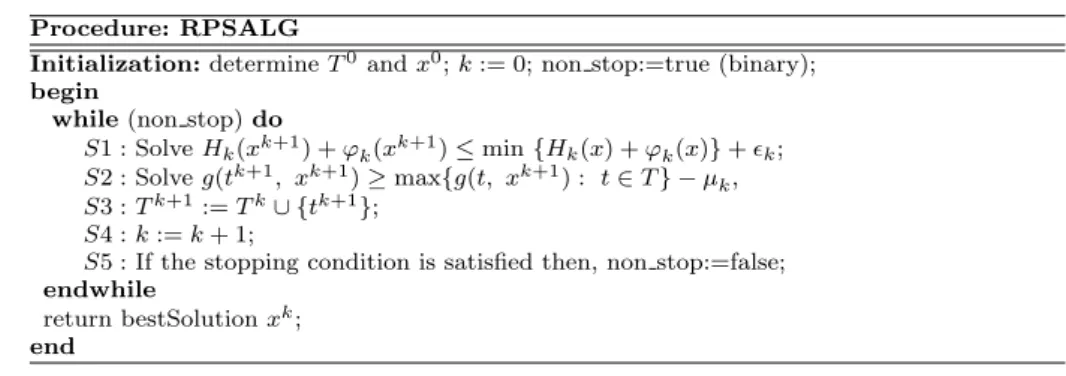
whereθbelongs to some family of penalty functions, and{γk}and{δk}are appro-priated sequences of positive scalars;Gk(x) is a penalty function for approaching of the feasible set of the discrete subproblem (Pk),i.e.{x∈Rn:g(t, x)≤0, t∈Tk}. RPSALG algorithm for solving (2) is described in Table 2, where {k}and{µk} denote two sequences of positive tolerances such thatk↓0 andµk↓0.
Table 2 RPSALG general framework
Procedure: RPSALG
Initialization:determineT0 andx0;k:= 0; non stop:=true (binary);
begin
while(non stop)do
S1 : SolveHk(xk+1) +ϕk(xk+1)≤min{Hk(x) +ϕk(x)}+k;
S2 : Solveg(tk+1, xk+1)≥max{g(t, xk+1) : t∈T} −µk,
S3 :Tk+1:=Tk∪ {tk+1}; S4 :k:=k+ 1;
S5 : If the stopping condition is satisfied then, non stop:=false;
endwhile
return bestSolutionxk;
Unfortunately there is not much software for SIP. In this paper we compare RP-SALG with NSIPS, the unique solver publicly available so far for solving SIP prob-lems. NSIPS is a set of solvers for semi-infinite programming problems designed without assumptions of convexity. NSIPS uses the SIPAMPL software package, which allows the codification of semi-infinite programming problems in AMPL and includes a database with a large battery of coded SIP problems (see [32] and the SIPAMPL manual1for additional information). NSIPS is publicly available on the NEOS server platform2. NSIPS includes four solvers: a discretization solver, a penalty technique solver, a sequential quadratic programming solver (SQP), and an infeasible quasi-Newton interior point solver. Some of them need to use com-mercial software NPSOL [18].
Of all the solvers included in NSIPS only the penalty technique solvers are considered in the article. Penalty methods include two versions based on a quasi-Newton method applied to penalty functions. The first method solves the uncon-strained problem, and it is based on penalty functions (several penalty functions can be selected), and no reference to Lagrange multipliers is made. The second one solves the unconstrained problem using two possible options, namely an Aug-mented Lagrangian penalty function or a multiplier penalty function.
The paper is organized as follows. Section 2 describes different versions of RP-SALG for problems with a unique block of constraints. Section 3 analyzes, from a computational efficiency point of view, implementations of RPSALG based on optimal gradient algorithms and variable metric schemes. Section 4 proposes stop-ping rules for both auxiliary optimization subproblems. Section 5 adapts RPSALG to problems with constraints in blocks. Section 6 compares the numerical results obtained for two particular implementations of RPSALG, and for two particular NSIPS solvers on a large collection of test problems. Finally, Section 7 provides some conclusions.
2 Versions of RPSALG
The implementation of RPSALG for the problem (P) formulated in (2) depends on the optimization algorithms used in steps S1 andS2 (see Table 2), and also on the regularizing convex function ϕ, the penalty functionθ, and the couple of sequences of positive scalars{γk} and{δk}. Notice that for each choice of these parameters we have a different instance of RPSALG.
Thus, once a standard algorithm has been chosen for solvingS1 (e.g., a Gradient-type, a Newton-Gradient-type, or a Quasi-Newton-type algorithm), the following question arises: how to solve efficiently the non-convex program in stepS2 when either the dimension ofT is greater than one or the constraint functions are non-standard? A sensible answer to this question consists of using the so-called Extended Cutting Angle Method (ECAM), a global optimization procedure for Lipschitz programs that allows us to solve the subproblemsS2 regardless of the dimension ofT. To the authors’ knowledge, the use in this article of global optimization software, such as ECAM, to solve the non-convex program at the step S2 in algorithms based on Remez’s approximation is an innovation in the field.
1 http://plato.la.asu.edu/ftp/sipampl.pdf 2 http://www.neos-server.org/neos/
2.1 The choice of the regularizing convex functionϕ
The most relevant choice concerns the regularizing convex function ϕ, as it de-termines the convergence behavior of the corresponding variants of our method. In this paper we consider two versions of RPSALG, named RPSALG1 and RP-SALG2, that use different regularizing convex functions,ϕ1andϕ2,guaranteeing the strong convexity of the objective function in the unconstrained convex problem (3). Consider the regularizing functionsϕ1, ϕ2:Rn→R defined by
ϕ1(x) =kxk2, for >0, andϕ2(x) =1
2kx−xk 2
, for x∈Rn,
i.e. the Tihonov and the Moreau-Yosida regularizing functions, respectively. In RPSALG1 we associate with a given positive sequence{k}such thatk &0 the sequence of regularized subproblems
(Pk1) min{Hk(x) +ϕ1k(x) : x∈R n
}, k= 1,2, ..., whereϕ1k(x) :=kkxk2, k= 1,2, ...
In RPSALG2 we consider the sequence of regularized subproblems
(Pk2) min{Hk(x) +ϕ2k(x) : x∈Rn}, k= 1,2, ...., (6) where ϕ2k(x) := 12 x−x k−1 2
, k = 1,2, ..., with xk−1 denoting an approximate solution of (Pk2−1).
2.2 The choice of the penalty functionθ
In order to guarantee the convergence of RPSALG, the penalty function θ:R→ R+ in (5) is required to be C1, convex, non-decreasing, non-constant and with limu→−∞θ(u) = 0.These conditions are satisfied by well-known penalty functions as the following: θ1(u) = log(1 + exp(u)), θ2(u) = 2−1(u+pu2+ 4), θ3(u) = 0, u≤ −1, 1 4(u+ 1) 2 ,−1< u <1, u, u≥1, θ4(u) = 1 2(u +)2 , whereu+:= max{u,0}, θ5(u) = (u+)3, and θ6(u) = exp(u).
The assumptions onθ entail θ∞(−1) = 0 andθ∞(1)>0, where θ∞ denotes the asymptotic function of θ,i.e. epi(θ∞) = (epiθ)∞ (the so-called recession cone of the epigraph ofθ).
2.3 The choice of the positive sequences{γk}and{δk}
Once the regularizing function has been fixed, each triplet (θ,{γk},{δk}) in the expression Gk(x) = γk |Tk| X t∈Tk θ(g(t, x)δk) δk
determines a different instance of RPSALG. To ensure convergence, we consider the following conditions involving a sequence of integer numbers {mk}such that mk≥ |Tk|, k= 1,2, ...:
(a) θ∞(1)<+∞,limk→∞γk/δk = 0,and limk→∞γk/mk= +∞.
(b) θ∞(1) = +∞,limk→∞γk/δk= 0,andγk/mk> ε∀kand a certain ε >0. (c) θ∞(1) = +∞,limk→∞δk = +∞, γk/mk > ε∀k and a certainε >0, {γk/δk}
is bounded, andθ(0) = 0 or the Slater condition holds. Observe that the three conditions (a), (b) and (c) imply
lim
k→∞γk= limk→∞δk= +∞.
The convergence of RPSALG1 derives from the following result (for RPSALG2 no counterpart is still available):
Theorem 1 [1, Theorem 3.1] If the triplet(θ,{γk},{δk})satisfies at least one of the
conditions (a), (b), (c), then the sequence n
xk
o
built by RPSALG1 is bounded and each limit point of this sequence is an optimal solution of(P).
With respect to the choice of the sequences {γk} and {δk} three cases are considered in our implementation. If we take mk := |T0|+k, we can verify the following statements:
i) γk := (mk)1.5 and δk := (mk)2.5 satisfy (a), (b) and (c). Then, any triplet (θ,{γk},{δk}) withθ∈ {θ1, θ2, θ3, θ4, θ5}can be used.
ii) γk :=mkandδk:= (mk)1.5satisfy (b) and (c). Then, any triplet (θ,{γk},{δk}) with θ∈ {θ4, θ5, θ6}can be used.
iii) γk =δk =mk satisfy (c). Then, any triplet (θ,{γk},{δk}) withθ∈ {θ4, θ5}, or θ=θ6together the Slater condition can be used. Nevertheless, Slater condition will not be taken into account in our analysis because it is difficult to be checked.
3 Implementing RPSALG
As we have seen, each triplet (θ,{γk},{δk}) determines a different instance of RP-SALG. In this section, we compare the implementations corresponding to cases i), ii) and iii), in which RPSALG1 converges. Nevertheless, some considerations must be taken into account. Indeed, the standardization of floating point arithmetics fol-lows the IEEE 754 standard. This standard has some major shortcomings. One of them is that it does not specify the behavior of standard transcendental functions so as the exponential function. As J.M. Muller states in [26], some transcenden-tal functions are even very badly implemented in common run-time libraries that
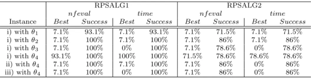
produce wrong results on some arguments. Thus, the defective results generated could seriously affect the numerical stability of the implementations. In addition, the lack of an exact definition of the results to be returned by standard libraries prohibits portability over different platforms. These drawbacks suggest not to use the penalization functionsθ1andθ6in our implementation of RPSALG. However, in order to emphasize the previous comments on numerical instability we have included the results of the functionθ1in Table 3, where we can see that it has the worst computational behavior from the point of view of successfully completing the program run. On the other hand, penalty functions θ4 andθ5 have a simi-lar performance. For this reason, since our purpose is to show the best penalty function, in Table 3 we only compareθ4with θi,i= 1,2,3.Tests with θ5 andθi, i= 1,2,3,have shown similar results on RPSALG.
3.1 Choosing an efficient version of RPSALG
The benchmark results are generated by running RPSALG1 and RPSALG2 on the set of test problems described in [21]. Then, we report information of interest for each instance from its performance profile (see Appendix for a summary or [14] for complete description) with respect the number of function evaluations and the CPU-time. From Table 3 we can compare the instances with the probability of win over the rest, Best, and the probability of success,Success, in solving the test problems with respect the number of function evaluations, nfeval, and the CPU-time,time.
Table 3 Performance profile results for instance evaluations
RPSALG1 RPSALG2
nf eval time nf eval time
Instance Best Success Best Success Best Success Best Success
i) withθ1 7.1% 93.1% 7.1% 93.1% 7.1% 71.5% 7.1% 71.5% i) withθ2 7.1% 100% 7.1% 100% 7.1% 86% 7.1% 86% i) withθ3 7.1% 100% 0% 100% 7.1% 78.6% 0% 78.6% i) withθ4 93.1% 100% 100% 100% 71.5% 78.6% 78.6% 78.6% ii) withθ4 7.1% 100% 7.1% 100% 7.1% 86% 0% 86% iii) withθ4 7.1% 100% 0% 100% 7.1% 86% 0% 86%
As we can see, the case i) with functionθ4is the best for all options. It requires less functions evaluations in the 93.1% of the cases with RPSALG1 (with an 100% of success), and in the 71.5% of the cases with RPSALG2 (78.5% of success). Moreover, it is the best option for CPU-time since it spends less time in the 100% of the cases with RPSALG1 (100% of success), and in the 78.6% of the cases with RPSALG2 (78.6% of success). So, we shall use the case i) with functionθ4 in all RPSALG implementations.
3.2 Building a starting gridT0
As explained in Section 1, we confine ourselves to consider ordinary convex SIP problems of the form (2) such that T is a compact metric space, the objective functionf:Rn→Ris convex onRn and level bounded onC={x∈Rn:G(x)≤ 0}, g:T ×Rn →R is continuous, and the constraint functionsgtare convex on Rn for all t ∈ T; we also assume that the involved functions, f and gt, t ∈ T, areC1. These assumptions guarantee that the optimal set of (2) is nonempty and compact (by the same argument as [1, Prop. 2.1]). Moreover, by [1, Lemma 3.1], there exists a finite nonempty subset T0 ⊂ T such that f is level bounded on C0 := {x ∈ Rn : G0(x) ≤ 0}, with G0(x) := max{gt(x) : t ∈ T0}. There are some particular cases in which the setT0is easily obtainable. For instance, when T = cl intT ⊂Rm andβr&0,since dist (T∩βrZm, T)→0,it is possible to take the regular gridT0=T∩βrZm for sufficiently larger(see [1, Remark 3.1]).
When T is either a full dimensional closed convex sets or the finite union of pairwise disjoint sets of this class (typically a box or the union of finitely many disjoint boxes, as it happens in almost all test problems), thenT = cl intT by the accessibility lemma.
WhenT has a finite number of isolated elements (indices), then they must be included inT0.So, it is easy to get a starting gridT0whenever T is the union of a finite set with finitely many pairwise disjoint boxes.
3.3 Solving the programs at stepS1
The aim of this subsection is to discuss the optimization methods allowing to solve efficiently the subproblems
(Pk1) inf{Hk(x) +kkxk2 : x∈Rn}, k= 1,2, ..., and (Pk2) inf{Hk(x) + 1 2 x−x k−1 2 : x∈Rn}, k= 1,2, ...,
whereHk(x) =f(x) +Gk(x).These problems have the common form
inf{f(x) : x∈Q},
wheref is a strongly convex objective function C1on Q=
Rn.When the number n of variables is too large we cannot use Newton type methods but only gradi-ent based methods. We summarize now, very shortly, the accelerating gradigradi-ent methods based on Nesterov’s ideas. Let Q be a closed convex set in Rn and let f : Rn → R∪ {+∞} be a proper lower semicontinuous convex function, C1 on Q.We suppose the existence of a global minimizer x∗ of f on Qand that∇f is globally Lipschitz onQwith Lipschitz constantL. This constant must be known since it is used in the construction of Nesterov-type method. More precisely, if {xk}is a sequence given by such an algorithm that we shall denote OGA (optimal gradient algorithm), then there exists a constantD(x∗, x0), depending onx∗ and the starting pointx0 such that
Furthermore, Nesterov [27] has shown that this estimate is ”optimal” for the class of convex C1 functions for which the gradient is globally Lipschitz (this last as-sumption is essential). It is worthwhile to note that Q must be ”simple” in the following sense: all the formulas in OGA are given by analytic formulas, without any subroutine for solving a minimization subproblem, so that (7) is really a com-plexity estimation. As examples of ”simple” setsQwe have Euclidean balls, affine sets, half-spaces, box constrained sets, simplex sets, etc. This kind of “optimal methods” have been extended with different versions to constrained optimization independently by Nesterov [27] and by Auslender and Teboulle [2] for “simple” feasible sets.
Since the comparative study tackled in this paper requires to solve (Pk1) and (Pk2) for the convex SIP problems collected at the SIPAMPL database, where Q = Rn, n is small, and the objective functions are very general (so that it is not possible to give analytic formulas), OGA methods are not so advantageous in this framework. We illustrate this sentence analyzing the particular case of linearly constrained convex SIP problems, i.e. problems as (P) in (2) withg(t, x) = hat, xi −bt,withat∈Rn andbt∈R,for allt∈T .The continuity ofgon T×Rn entails thatt7→atis continuous on the compact set T,so that
µ:= sup t∈T
katk is attained.
Proposition 1 Let θ:R→R+ be a C1,convex, non-decreasing, non-constant
func-tion such thatlimu→−∞θ(u) = 0 andθ0 is globally Lipschitz on Rwith constant α.
Assume thatL0 is a Lipschitz constant for∇f.Then∇ Hk+ϕ1k
and∇ Hk+ϕ2k
,
are globally Lipschitz with constantsL1 andL2 given by
Lk1=L0+ 2k+αγkδkµ2 andLk2=L0+ 1 +αγkδkµ2,
respectively.
Proof: Let θ be as above, with Lipschitz constant α. Given an affine function h(x) =δ(ha, xi −b),withδ≥0, a∈Rn,andb∈R,we have∇θ(h(x)) =δθ0(h(x))a. Thus, for any two pointsx, y∈Rn,one has
k∇θ(h(x))− ∇θ(h(y))k=δkakθ0(h(x))−θ0(h(y)) ≤αδkak kh(x)−h(y)k ≤αδ2kak2kx−yk,
so that∇(θ◦h) is globally Lipschitz onRn with constantαδ2kak2.Hence,
∇Gk(x) = γk |Tk| P t∈Tk∇θ(δkg(t, x)) δk is globally Lipschitz too, with Lipschitz constant αγkδk
|Tk|
P
t∈Tkkatk
2 ≤
αγkδkµ2. Thus, ∇Hk(x) = ∇f(x) +∇Gk(x) is globally Lipschitz with Lipschitz constant
L0+αγkδkµ2.
The penalty functions θ1 andθ2 satisfy the assumptions of Proposition 1 be-cause they are C2 with 0 ≤ θ001(u) ≤ 14 and 0 ≤ θ
00
the non-C2 functionsθ3 andθ4 satisfy the assumptions as their derivatives have Lipschitz constants equal to 2 and 1,respectively. Observe that the derivatives of θ5 andθ6 are not globally Lipschitz. Concerning the objective function f,∇f is Lipschitz with Lipschitz constantL0= 0 wheneverf is linear (i.e. in linear SIP).
Nevertheless, in practice, OGA is inconvenient for solving the problems con-sidered because the product γkδk tends to infinity as the number of iterations increases so thatLki →+∞ as k →+∞, i= 1,2. Indeed, in each iteration new points must be calculated through steps whose length depends on 1/Lki, which tends to zero ask→+∞, this makes OGA increasingly slow and inefficient. This phenomenon is illustrated in the Tables 4 and 5, corresponding to Example 1 below. For this reason, we propose to use the Limited-memory Broyden-Fletcher-Goldfarb-Shanno method [28] to solve the subproblems in Step 1 of Table 2. This is a quasi-Newton method (denoted by QN in the sequel) for unconstrained opti-mization that iteratively finds a minimizer by approximating the inverse Hessian matrix using information from last iterations, which drastically saves the memory storage and computational time for large-scaled problems.3
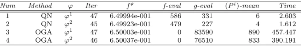
Example 1 Consider the well-known test problem from linear semi-infinite liter-ature consisting on computing the polynomial of degree less than n that best approximates the tangent curve over [0,1] in theL1norm whose exact solution is known (see [21]). minimize f(x) =Pn i=1 xi i subject to:−Pn i=1xit i−1≤ −tant, t∈[0, 1].
We solve it forn= 3, taking the penalization functionθ2and the positive sequences γk:= (|T0|+k)1.5 andδk= (|T0|+k)2.5.
We can observe the results in Table 4 and Table 5. The columnMethodin Table 4 indicates the use of QN or OGA methods,ϕindicates the regularized function which has been used, Iter indicates the number of major iterations required, f∗ represents the optimal value obtained by RPSALG,f-eval is the number of objec-tive functions evaluations,g-evalis the number of gradient evaluations, (Pi)-mean
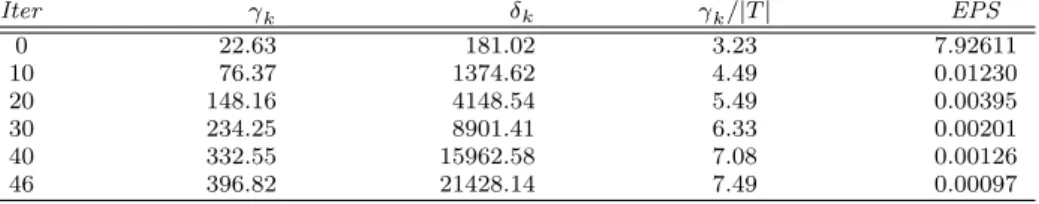
is the average of the iterations performed at each major iteration in the problems (Pki),i= 1, 2 andTime is the CPU time in seconds. On the other hand, Table 5 represents the evaluation of the numbersγk,δkandγk/|T|for the problem number 4 in Table 5, andEPS indicates the stopping criterion evaluation.
Table 4 Results and CPU time for the tangent sample with precision= 0.001
Num Method ϕ Iter f* f-eval g-eval (Pi)-mean Time
1 QN ϕ1 47 6.49994e-001 586 331 6 2.603
2 QN ϕ2 45 6.49923e-001 479 227 4 1.612
3 OGA ϕ1 47 6.50003e-001 0 83590 890 457.447
4 OGA ϕ2 46 6.50037e-001 0 76510 833 390.191
In Table 5 we can see the inconvenience of using OGA algorithm since the product γkδk tends to infinity as the number of iterations increases. In Table
4 we can compare the results of the different versions of the RPSALG and the advantages of using a Quasi-Newton method for solving subproblems in Step 1 of Table 2. Also, we can see that the use ofϕ2as the regularizing function allows one to reduce the CPU time in comparison with the use ofϕ1.
Table 5 {γk}and{δk}for the problem 4 in Table 4
Iter γk δk γk/|T| EPS 0 22.63 181.02 3.23 7.92611 10 76.37 1374.62 4.49 0.01230 20 148.16 4148.54 5.49 0.00395 30 234.25 8901.41 6.33 0.00201 40 332.55 15962.58 7.08 0.00126 46 396.82 21428.14 7.49 0.00097
3.4 Solving the programs at stepS2
The subproblems to be solved in Step 2 consist of finding the optimal set of g(·, x) :T →Rfor somex∈Rn.Assume thatg(·, x) is C1onT,for allx∈
Rn,and denoteµ:= maxt∈Tk∇tg(t, x)k ∈R.Then, givent1, t2 ∈T,there existsλ∈]0,1[ such that
|g(t1, x)−g(t2, x)|=|h∇tg((1−λ)t1+λt2, x),(t1−t2)i| ≤µkt1−t2k,
so thatg(·, x) is Lipschitz continuous onT with Lipschitz constantµ.
Assume further thatT is a convex polyhedron (typically, it is a box). Then we have to find the solution set of a problem of the form
inf{f(x) :x∈S}, (8)
wheref is Lipschitz continuous andS is a convex polyhedron.
In all the implementations of RPSALG considered in this paper we use an extension of the Cutting Angle method of Bagirov and Rubinov [3], due to Beliakov ([6],[7],[8],[9],[10]) and called Extended Cutting Angle Method (ECAM in short), in order to solve this very hard optimization problem. In ECAM the objective function is assumed to be Lipschitz continuous and it is optimized by building a sequence of piecewise linear underestimates. ECAM is inspired in the classical Cutting Plane method by Kelley [25] and Cheney and Golstein [12] to solve linearly constrained convex programs of the form (8), whereSis the solution set of a given linear system andf :Rn→R is convex. Sincef is lower semicontinuous, it is the upper envelope of the set of all its affine minorants, i.e.
f= sup{h : haffine function,h≤f}. (9)
Indeed, it is enough to consider in (9) the affine functions of the form h(x) = f(z)+hu, x−zi,whereu∈∂f(z) (the subdifferential offatz∈Rn), the graph ofh being a hyperplane which supports the epigraph offat (z, f(z)).Letx1, ..., xk∈S
be given and consider the affine functions hj(x) =f(xj) + uj, x−xj,for some uj∈∂f xj , j= 1, ..., k.The function fk := max j=1,...,kh j (10)
is a convex piecewise affine underestimate of the objective function f, in other words, a polyhedral convex minorant off.Thek-th iteration of the Cutting Plane method consists of computing an optimal solutionxk+1of the approximating prob-lem inf{fk(x) :x∈S}which results of replacingf withfk in (8) or, equivalently, solving the linear programming problem inRn+1
infnxn+1:x∈S, xn+1≥hj(x), j= 1, ..., k
o
, (11)
wherex= (x1, ..., xn).Then the next underestimate off, fk+1:= max
n
fk, hk+1 o
, is a more accurate approximation tof,and the method iterates.
The Generalized Cutting Plane method for (8), wheref:Rn→Ris now a non-convex function while S = nx∈Rn+:
Xn
i=1xi= 1
o
is the unit simplex, follows the same script, except that the underestimatefk is built using the so-calledH -subgradients (see [30]) instead of ordinary -subgradients, so that minimizingfkonS is no longer a convex problem. The Cutting Angle method ([3],[4]), of which ECAM is a variant, is an efficient numerical method for minimizing the underestimates when f belongs to certain class of abstract convex functions. Assume that f is Lipschitz continuous with Lipschitz constantM >0 and take a scalarγ≥M.Let x1, ..., xk∈S be given. Forj= 1, ..., k,we define thesupport vector lj∈Rn by
lji := f(x j) γ −x
j
i, i= 1, . . . , n, (12) and thesupport function hj by
hj(x) := min i=1,...,n(f(x j )−γ(xji−xi)) = min i=1,...,nγ(l j i +xi). (13) Since the functionshj are concave piecewise affine underestimates off (i.e. poly-hedral concave minorants of f), the underestimate fk defined in (10) is now a saw-tooth underestimate of f and its minimization becomes a hard problem as (11) is no longer a linear program.ECAM locates the set Vk of all local minima of the functionfk which, after sorting, yields the set of global minima offk (see [8] and [9] for additional information). A global minimumxk+1offk is aggregated to the setnx1, ..., xk
o
and the method iterates withfk+1:= max
n
fk, hk+1 o
.
Remark 1 Notice that the transformation of variables 1) ¯xi=xi−ai, i= 1, . . . , n, d=Pni=1(bi−ai) with ¯xi≥0 and
Pn
i=1¯xi≤d 2) zi= x¯di, i= 1, . . . , n,zn+1=Pni=1zi,
allows us to substitute the program
min{f(x) :x∈[a, b]} by the following one:
min{g(z1, . . . , zn+1) : (z1, . . . , zn+1)∈S}, whereS denotes the unit simplex inRn+1.
4 Stopping rules
4.1 Stopping rule for programs at the stepS1
SinceHk isC1, any usual convergent gradient method will provide the iteratexk in a finite number of steps if suitable stopping rules are adopted.
The regularized objective functions
Hregi
k (x) :=Hk(x) +ϕik(x), i= 1,2; k= 1,2, ....,
are strongly convex and so, they have a unique global minimizeryik. According to S1 in Table 2, for eachk,(Pki), i= 1,2,has to be solved within the errork,with k&0, i.e.xk must satisfy
Hregi
k (x k
)≤Hregi
k (x) +k, ∀x∈Rn, i= 1,2; k= 1,2, ... (14)
Stopping rule for (Pk1) in RPSALG1: According to [1, Remark 3.2], (14) will be satisfied, i.e. Hk(xk) +k x k 2 ≤Hk(x) +kkxk2+k ∀x∈Rn. (15)
provided that we use the stopping rule ∇Hk(x k) + 2 kxk ≤ √ 2k, (16) where ∇Hk(xk) =∇f(xk)+ γk |Tk| X t∈Tk θ0(δkgt(xk))∇gt(xk)
is obtained by the chain rule.
Stopping rule for (Pk2)in RPSALG2:Now (14) will be satisfied, i.e. Hk(xk) +1 2 x k −xk−1 2 ≤Hk(x) + 1 2 x−x k−1 2 +k ∀x∈Rn. (17)
provided that we use the stopping rule ∇Hk(x k) + xk−xk−1 ≤ √ k. (18)
In fact, the functionHreg2
k is strongly convex with modulus 1 [20, IV, Theorem 4.3.1], and applying (18) and [20, IV, Theorem 4.1.4] to the couple of pointsxk andy2k where{yk2}= argminRnH
reg2 k (and so,∇H reg2 k (y k 2) = 0n): x k− y2k 2 ≤D∇Hreg2 k (x k )− ∇Hreg2 k (y k 2), xk−yk2 E ≤ ∇H reg2 k (x k )− ∇Hreg2 k (y k 2) x k −yk2 = ∇H reg2 k (x k ) x k −y2k ≤√k x k −yk2 ,
entailing x k− y2k ≤ √ k.Moreover, by convexity, Hreg2 k (x k )≤Hreg2 k (y k 2)− D ∇Hreg2 k (x k ), xk−y2k E ≤Hreg2 k (y k 2) + ∇H reg2 k (x k ) x k− yk2 ≤Hreg2 k (y k 2) + √ k √ k, and we get (17).
Proposition 2 Assume that the triple(θ,{γk},{δk})satisfies at least one of the
con-ditions (a), (b), (c) in Theorem 1. Letξ andη be given positive numbers (tolerances) and let
n
xk
o
be the sequence generated by RPSALG 1. Then ∇Hk(x k ) ≤ξ andG(x k )≤η (19)
holds for somek∈N.
Proof:We can assume without loss of generality (w.l.o.g., in short) thatnxk
o is convergent. It is sufficient to show that limk→∞
∇Hk(x k) = 0 and limk→∞G(x k)≤ 0.
Let x∗= limk→∞xk.By Theorem 1x∗ is an optimal solution of (P).On the one hand, taking limits in (16) ask→ ∞,we get limk→∞
∇Hk(x
k)
= 0.On the other hand,G(x) = max{gt(x) :t∈T}is a convex finite-valued function, so that it is continuous and, so, limk→∞G(xk) =G(x∗)≤0.
Remark 2 The proof of Theorem 1 does not make use of the differentiability of the functions gt, t ∈T (see [1] for the details) Nevertheless, if gt is not differen-tiable, the same may happen withGk andHk, so that the new iterate xk could be non-approachable by gradient methods and the stopping rules (16) and (18) may not apply. So, convergence of RPSALG1 is conditioned to the fact that all the constraint functions are continuously differentiable at the elements of the sequence n
xk
o
built by RPSALG1, a condition which cannot be checked a priori.
4.2 Global stopping rule for RPSALG1
Theorem 1 established the existence of a subsequence of iterates {xk}k∈K such that limk∈K, k→∞xk=x∗, wherex∗ is optimal for problem (P) in (2). In [1], the Lagrangian dual of (P) is studied by considering the dual pair formed by:
a)C(T): the Banach space of real-valued continuous functions onT, equipped with the maximum norm
khk= max{|h(t)|:t∈T}.
b) M(T) : the topological dual of C(T), i.e. the space of all the finite signed Borel measures onT, embedded with the total variation norm.
c) The pairing
hσ, hi= Z
T
h(t)σ(dt) withσ∈ M(T) andh∈ C(T).
In [1, Section 4], a sequence of discrete measures {σk}k∈K associated with {xk}k∈K is introduced by means of the expression
σk := γk Tk X t∈Tk θ0(g(t, xk)δk)αt, (20)
where αt is the Dirac measure concentrated att, i.e. for any continuous function h∈ C(T)
hαt, hi=h(t).
Assuming that the objective function f : Rn →R is convex on Rn and level bounded on the feasible set C:={x∈Rn :G(x)≤0}, that the Slater constraint qualification holds, and that∇g(., .) exists and is continuous onT×Rn, Theorem 4.2 in [1] establishes the existence of a subsequence{σk}k∈K0, K0 ⊂K, which is
weak*-convergent to a measureσ∗.The measureσ∗is an optimal solution for the Lagrangian dual problem (D) given in [1, (47)] and satisfies
σ∗, g(·, x∗) = 0.
Then, applying for instance [11, Proposition 2.24(iii)], we have
lim k∈K0, k→∞hσ k , g(·, xk)i= σ∗, g(·, x∗) = 0.
Inspired by this fact we can use the following global stopping rule: hσ k , g(·, xk)i = γk Tk X t∈Tk θ0(g(t, xk)δk) gt(x k ) ≤η, (21)
whereη >0 is a tolerance parameter.
In the particular case of linearly constrained convex SIP, i.e.g(t, x) =ha(t), xi− b(t),if we useθ(u) =θ4(u) =12(u+)2,the stopping rule (21) becomes
γkδk Tk X t∈Tk (hDa(t), xk E −b(t)i+)2≤η. (22)
5 Adapting RPSALG to constraints in blocks
Some SIP problems arising in practice can be formulated as
(P0)f∗= inf{f(x) : gi(t, x)≤0, t∈Ti, i= 1, ..., m}, (23)
whereTiis a (possibly degenerate) compact interval inRdi, i= 1, ..., m, f :Rn→R is convex onRnand level bounded on the feasible setC:={x∈Rn:Gi(x)≤0, i= 1, ..., m}, with Gi(x) := max{gi(t, x) : t∈ Ti}. Assume that for each i= 1, ..., m, gi : Ti×Rn → R is continuous, and the functions gi(t,·) are convex on Rn for all t ∈Ti. Assume also that the involved functions, f and gi(t,·), t∈ T,are C1.
We shall now describe a procedure to reformulate (P0), when Ti is a (possibly degenerate) interval for all 1, ..., m,with a unique index set, in three steps which preserve the objective functionf and the feasible setC.
Step 1: Embedding all index sets in the same space.
Let d:= max{di:i= 1, ..., m}andTi= Y j=1,...,di αij, βij , αij≤βij, j= 1, ..., di. If di < d, we define αij, βij := [0,1], j = di+ 1, ..., d, Tei = Ti×[0,1]d−di and e
gi:Tei→Rsuch thategi(t, s, x) =gi(t, x) for all (t, s, x)∈Ti×[0,1] d−di×
Rn.Then, we can replacegi(t, x) in (P) byegi(t, s, x),whereegienjoys the same properties as
gi.At the end of Step 1, we have an optimization problem of the form (P1)f∗= inf{f(x) : gi(t, x)≤0, t∈Ti, i= 1, ..., m}, where all the index setsTihave the same dimension.
Step 2: Unifying the index sets.
Assume that Ti = Y j=1,...,d αij, βij , αij ≤βij, i = 1, ..., m.Given i∈ {1, ..., m}
and j ∈ {1, ..., d}, define hij : R → R such that hij(λ) = (1−λ)αij+λβij. For i∈ {1, ..., m},let hi :Rd →Rd be the affine mapping such that hi(λ1, ..., λd) =
hi1(λ1), ..., hid(λd)
. Since Ti = hi
[0,1]d,defining egi(s, x) := gi(hi(s), x), we can replace the constraint system in (P) with { egi(s, x)≤0, s∈T, i = 1, ..., m}, where T = [0,1]d is the common index set of all blocks of constraints. So, Step 2 provides a reformulation of (P1) of the form
(P2)f∗= inf{f(x) : gi(t, x)≤0, i= 1, ..., m, t∈T},
whose constraint functions satisfy the same properties as those in the initial model (P).
For most SIP problems arising in functional approximation Steps 1-2 are usu-ally unnecessary as the index setsTi coincide.
Example 2 Consider the problem consisting of computing a best uniform approx-imation from above to a given functionh: [α, β]→R, α < β, by means of poly-nomials of degree less than n−1,with n >2,under the condition that they are non-decreasing and convex on [α, β].Since the unknown polynomial Pn−1
i=1 t i−1
xi can be represented by its vector of coefficients (x1, ..., xn−1),denoting byxn the uniform error bound, the problem to be solved is
(P2)f∗= inf{f(x) : gi(t, x)≤0, i= 1, ...,5, t∈[α, β]}, wherex= (x1, ..., xn), f(x) =xn,and the constraints are:
◦Approximation from above:g1(t, x) =h(t)−Pni=1−1t i−1x i≤0. ◦Monotonicity:g2(t, x) =−Pn−1 i=1 (i−1)t i−2x i≤0. ◦Convexity:g3(t, x) =Pni=1−1(i−1) (i−2)t i−3x i≤0.
◦xn is a lower uniform error bound:g4(t, x) =−Pni=1−1ti−1xi−xn+h(t)≤0. ◦xn is an upper uniform error bound:g5(t, x) =Pni=1−1ti−1xi−xn−h(t)≤0.
Step 3: Reduction to a unique block.
Defining g(t,·) := max{gi(t,·), i= 1, ..., m},we get the following reformulation of (P2) :
(P3)f∗= inf{f(x) :g(t, x)≤0, t∈T}.
Since gi :T ×Rn →R is continuous and the functions gi(t,·) areC1 and convex onRn for allt∈T andi= 1, .., m,(P3) satisfies the same assumptions required to the problem (P) in (2), except the possible lack of differentiability of gt at those pointsx∈Rn whose correspondingset of active indices, defined as
It(x) = i∈1, ..., m:gi(t, x) = max j=1,...,mgj(t, x) ,
is not a singleton (i.e. such that max{gi(t, x), i= 1, ..., m}is attained at more than one index). Thus, the set
[
1≤i<j≤m
x∈Rn:gi(t, x) =gj(t, x) . (24)
contains all points wheregtfails to be C1.When solving (P3) with RPSALG, the failure of theC1property ofg
tatxkfor somet∈Tk entails the non-smoothness of the auxiliary problem (Pk1),which should be solved with some subgradient method (instead of a gradient one). Fortunately, the subdifferential ofHk atxk, ∂Hk(xk), can be easily computed through the closed formula (25), where convX stands for the convex hull ofX.
Proposition 3 Let (P0)be as in (23), the triple(θ,{γk},{δk})be as in Theorem 1,
andHk be defined as in (4) and (5). Then, givenxk∈Rn, ∂Hk(xk) =∇f(xk)+ γk |Tk| X t∈Tk θ0 gt xk convn∇gi(t, xk) :i∈It xk o . (25)
Proof.Lett∈T be given. By [20, Theorem 4.3.1 and Corollary 4.3.2] one has ∂(θ◦gt) (x) =θ0(gt(x))∂gt(x) =θ0(gt(x)) conv [ i∈It(x) ∇gi(t, x) . (26)
Observing that all functions in the right hand-side of the equation
Hk(x) =f(x)+ γk |Tk| X t∈Tk θ(gt(x)δk) δk
are finite-valued and convex, we can combine [20, Theorem 4.1.1] and (26) to obtain ∂Hk(xk) =∇f(xk)+ γk |Tk|δ k P t∈Tk∂θ(g(t, xk)δk) =∇f(xk)+ γk |Tk| P t∈Tkθ0 gt xk convn∇gi(t, xk) :i∈It xk o .
The unique possible drawback of RPSALG applied to (P3) is related with the stopping rule ∂Hk(xk)∩ξB6=∅(where Bdenotes the closed unit ball in Rn), the natural extension of
∇Hk(x
k)
≤ξ,which does not guarantee finite termination. If the constraints in (P0) are linear and non-repeated (as in Example 2), the sets
x∈Rn:gi(t, x) =gj(t, x) , i6=j, are hyperplanes and so the set in (24) is null. Actually, even though we may havegi(t,·) =gj(t,·) on some set of positive measure in artificial examples, in most convex SIP applications the constraints of (P3) areC1 almost everywhere for allt∈T.In that case, since the functionsGk andHk areC1 except on some subset of
[ t∈Tk [ 1≤i<j≤m x∈Rn:gi(t, x) =gj(t, x) (union of T k
null sets), these functions areC
1 almost everywhere for allt∈T. So, one can expect the convergence of RPSALG applied to (P3) provided at least one of the conditions (a), (b), (c) in Theorem 1 holds.
The convex SIP problem (P0) with blocks formed by a unique constraint (gi(t, x)≤0,such that|Ti|= 1) can be reformulated as (P3).WhenT1 is infinite while|Ti|= 1, i= 2, .., m,it can be convenient to replace (P0) by a suitable approx-imating problem withC1constraints. Indeed, letθ:
R→Rbe a non-decreasingC1 function suchθ(u) = 0 for allu≤0 andθ(u)>0 for allu >0 (conditions satisfied by the penalty functions θ4 and θ5); choose ”big” positive numbers M1, ..., Mm and consider the convex SIP approximating problem
(Pa)f∗= inf{f(x) + m X
i=2
Miθ(gi(x)) : g1(t, x)≤0, t∈T1},
where gi(x) stands for gi(t, x) as the latter function does not depend on t for i = 2, ..., m. Obviously, (Pa) has the same feasible set as (P0) and satisfies all assumptions required to the problem (P) in (2).
Example 3 Consider the convex SIP problem (P0) inR2[32, page 49] with objective functionf(x) =kxk2and constraintsg1(t, x) =tx1+t2x2≤0, t∈[0,1], g2(t, x) = x1+x2−10≤0 (t= 2),andg3(t, x) =−x1−x2−10≤0 (t= 3). Despite the fact thatT1= [0,1], T2={2}andT3={3}have different dimensions, we can replace T2 andT3 byT1,obtaining the following reformulation of (P0) :
(P3) f∗= inf{kxk2:gt(x)≤0, t∈[0,1]},
whose constraint function
gt(x) = max n
tx1+t2x2, x1+x2−10,−x1−x2−10
o
isC1except on the union of the straight lines
x∈R2: (t+ 1)x1+ t2+ 1 x2=−10 and x∈R2: (t−1)x1+ t2−1 x2=−10 (a null set).
The alternative approach consists of taking two big numbersM1>0 andM2>0 and a functionθ∈ {θ4, θ5},and replacing (P0) with
Observe that the linear constraints could be replaced by the non-smooth convex constraint|x1+x2| ≤10,getting the simpler approximating problem
inf{kxk2+M θ(|x1+x2| −10) :tx1+t2x2≤0, t∈[0,1]},
withM >0.The disadvantage of the latter problem is the failure of theC1property of the objective function on the parallel straight linesx1+x2=±10.
6 Numerical results
In this section we present the results of numerical experiments to compare the two versions of RPSALG with the penalty solvers included in NSIPS.
6.1 Options to the Solvers
As we know RPSALG can solve convex semi-infinite programs of class C1, with-out any limitation on the number of parametric and non-parametric constraints, the initial guess, and the dimension of T. The public version of NSIPS without using the NPSOL commercial software [18] cannot start an instance unless an ini-tial guess has been defined. Moreover, the index set of any parametric constraint is a one-dimensional interval. On the other hand, penalty methods in NSIPS in-clude two versions based on a quasi-Newton method applied to penalty functions. The first method solves the unconstrained problem, based on penalty functions (that can be chosen on three options), where no reference to Lagrange multipliers is made. The second one, in which an estimation of the Lagrange multipliers is made, solves the unconstrained problem using two possible options: an Augmented Lagrangian penalty function or a multiplier penalty function. For making a more streamlined presentation of the results we previously have tested all the option solvers and finally the two most efficient of them (for each penalty method) have been selected to be compared against the two versions of RPSALG by using the best option described in Table 3, i.e., case i) with functionθ4.
As penalty functions we have selected the following AMPL command options (indeed they are the penalty functions with integral representations in [32, (5.11) and (5.14)]):option nsips options ’method=penalty pf type=p1’andoption nsips options ’method=penalty m pf type=p1’. In this article we refer to this couple of selected methods as Penalty1 and Penalty2, respectively.
6.2 Test problems
A total of 71 semi-infinite test problems have been selected satisfying the con-vexity and differentiability hypothesis of RPSALG with an initial guess. The test problems have been selected as follows: 37 of them have been obtained from the SIAMPL database4 (numbers from 1 to 29 in Table 6 and from 50 to 57 in Tables 9, 10) and the remaining 34 problems have been generated by using the procedure described in [17]. In this latter case we can generate test problems with known solution and without limitations onnand dimT.
6.3 Computational results
The numerical experiments were carried out on a PC with Processor Intel(R) Core(TM)2 Duo CPU E8500, 3.16 GHz and 3.49 GB of RAM (MS Windows XP, professional). For comparing the different solvers on the same computer we have used the AMPL Student Version 20111121 (MS VC++ 6.0) to run NSIPS. The AMPL student version can be downloaded for free but it is limited to solve problems with 300 variables and a total of 300 objectives and constraints.
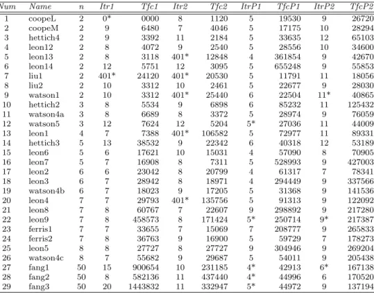
The numerical experiments are summarized in four tables. In Tables 6 and 7,
Num denotes the number assigned to the instance selected of the chosen solver,
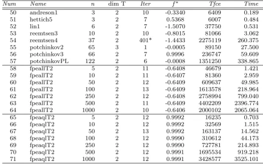
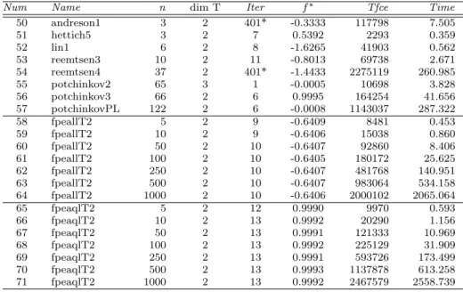
Nameindicates the name of the instance in SIAMPL database,n is the number of variables,Itr1 is the number of iterations required for RPSALG1,Tfc1 indicates the total number of functions and constraints evaluations for RPSALG1,Itr2 is the number of iterations required for RPSALG2,Tfc2 indicates the total number of functions and constraints evaluations for RPSALG2,ItrP1 is the number of it-erations required for Penalty1,TfcP1 indicates the total number of functions and constraints evaluations for Penalty1, ItrP2 is the number of iterations required for Penalty2,TfcP2 indicates the total number of functions and constraints eval-uations for Penalty2. In Tables 9 and 10 dimT represents the dimension of the space of parameters,f∗ the optimal value of the objective function,Tfce the total number of functions and constraints evaluations, andTimethe CPU time.
The results shown in the Tables 6 and 7 are compared in Table 8. The precise meanining of the entries in the latter table,ρs(1) (probability of success in solving a problem) andρ∗s(probability of win over the rest) is explained in the Appendix. The maximum number of iterations was limited to 400 and the precision is = 0.001 for all instances. If a solver needs more than 400 iterations to obtain a solution and/or the accuracy of the obtained solution is greater than the chosen value, then we will consider that the solver has failed in solving the problem. The failure of a solver is indicated with a star (∗), in the column that indicates the number of iterations of the corresponding solver.
Due to the mentioned limitations of the NSIPS, the computational results presented in the article have been divided in two cases:
i) Instances that satisfy the NSIPS limitations.We compare the total number of functions an constraints evaluations for the solvers RPSALG1, RPSALG2, Penalty1 and Penalty2 as described in Tables 6 and 7. For the sake of brevity and clarity, we have included the numerical results as performance profiles in Table 8. Figure 1 plots the performance profile of the results. From Table 8 we can compare the four solvers with respect to the probability of win over the rest,ρs(1), and the probability of success in solving a problem, ρ∗s.
ii) Instances that do not satisfy the NSIPS limitations. We compare the solvers RPSALG1, RPSALG2 for problems from 50 to 71 described in Tables 9 and 10, that do not satisfy the NSIPS limitations so we can only solve them by using the RPSALG versions. In Tables 9 and 10 the specific numerical results for the solvers RPSALG1, RPSALG2 with dimT >1 are described.
Table 6 Results for RPSALG1, RPSALG2, Penalty1 and Penalty2, dim T = 1, = 0.001, (∗) indicates the failure of corresponding solver
Num Name n Itr1 Tfc1 Itr2 Tfc2 ItrP1 TfcP1 ItrP2 TfcP2
1 coopeL 2 0* 0000 8 1120 5 19530 9 26720 2 coopeM 2 9 6480 7 4046 5 17175 10 28294 3 hettich4 2 9 3392 11 2184 5 33635 12 65103 4 leon12 2 8 4072 9 2540 5 28556 10 34600 5 leon13 2 8 3118 401* 12848 4 361854 9 42670 6 leon14 2 12 5751 12 3095 5 655248 9 55853 7 liu1 2 401* 24120 401* 20530 5 11791 11 18056 8 liu2 2 10 3312 10 2461 5 22677 9 28030 9 watson1 2 10 3312 401* 25440 6 22504 11* 40865 10 hettich2 3 8 5534 9 6898 6 85232 11 125432 11 watson4a 3 8 6689 8 3372 5 28974 9 76059 12 watson5 3 12 7624 12 5204 5* 27036 11 44009 13 leon1 4 7 7388 401* 106582 5 72977 11 89331 14 hettich3 5 13 38532 9 22342 6 40318 12 53189 15 leon6 5 6 17621 10 15031 4 57090 8 70905 16 leon7 5 7 16908 8 7311 5 528993 9 427003 17 leon2 6 6 23042 8 20799 4 61317 7 78341 18 leon3 6 7 28942 8 18971 4 294449 9 337566 19 watson4b 6 7 18023 9 17205 5 31368 9 141536 20 leon4 7 7 29793 401* 135756 5 91313 9 122092 21 leon8 7 8 60767 7 22607 9 298892 9 217280 22 leon9 7 8 458573 8 171424 5* 250714 9* 217387 23 ferris1 7 7 33655 7 15069 7 208777 9 265833 24 ferris2 7 8 36763 9 16900 5 59729 7 178273 25 leon5 8 8 27727 8 27727 9 304946 9 269204 26 watson4c 8 7 55682 9 29687 5 54011 9 205438 27 fang1 50 15 900654 10 231185 4* 42913 6* 167138 28 fang2 50 8 582136 11 437440 4* 44996 6 170520 29 fang3 50 20 1443832 11 332947 5* 44972 9 137194 7 Conclusions
This paper reports on the implementation of a penalty and smoothing method for solving convex semi-infinite programing problems inspired by the first algorithm of Remez, the so-called RPSALG. It is known that one of the main computational difficulties to solve semi-infinite programs comes from the non-convex optimization problem associated with the constraints, S2, which must be solved efficiently at each iteration. As an innovation of this paper, we tackle this problem with the so-called Cutting Angle Method, a global optimization procedure for solving Lipschitz programming problems. As far as we know, a global optimization software for solvingS2 has not been used before.
Two versions of RPSALG are proposed (RPSALG1 and RPSALG2), imple-mented in C++ and run on Visual C++ 6.0. We compare them with the best options of the two penalty methods solvers included in NSIPS, called Penalty1 (based on penalty functions where no reference to Lagrange multipliers is made) and Penalty2 (using an Augmented Lagrangian penalty function), and run on the student version of AMPL (with a maximum of 300 variables and a total of 300 objectives and constraints, and dimT = 1). We verify its performance by conduct-ing some numerical results with a set of test problems. All the results have been
Table 7 Results for RPSALG1, RPSALG2, Penalty1 and Penalty2, dim T =1= 0.001, (∗) indicates the failure of corresponding solver (Continued)
Num Name n Itr1 Tfc1 Itr2 Tfc2 ItrP1 TfcP1 ItrP2 TfcP2
30 ftpeallT1 5 8 23717 10 10486 3 68219 9 107806 31 ftpeallT1 10 8 38294 10 21980 4 104427 7 122150 32 ftpeallT1 15 9 64560 10 32020 4 128913 9 125002 33 ftpeallT1 20 9 74922 11 49486 4 149475 7 150263 34 ftpeallT1 25 9 113051 11 77726 3 134452 7 169104 35 ftpeallT1 50 8 204996 11 205008 4 152510 9 143445 36 ftpeallT1 100 9 370370 11 535044 3 217982 7 106212 37 ftpeallT1 150 9 631567 10 723818 4 72148 7 68182 38 ftpeallT1 200 9 888875 9 591287 3 59251 7 60756 39 ftpeallT1 250 9 1147834 8 564614 4 57262 7 62128 40 ftpeaqlT1 5 12 14823 13 14320 4 36017 9 53840 41 ftpeaqlT1 10 12 29001 13 24923 4 40330 10 62838 42 ftpeaqlT1 15 12 44718 12 32900 4 39372 10 66483 43 ftpeaqlT1 20 12 64793 13 49820 5 42169 9 67780 44 ftpeaqlT1 25 12 79442 13 63712 5 45696 8 50821 45 ftpeaqlT1 50 12 149173 12 109142 5 47843 9 67782 46 ftpeaqlT1 100 12 243641 12 222307 4 42026 10 60512 47 ftpeaqlT1 150 12 420680 12 325963 4 38261 9 68638 48 ftpeaqlT1 200 12 583250 12 444920 4 35394 7 47597 49 ftpeaqlT1 250 12 672318 12 573394 4 35427 7 48350
Table 8 Solvers evaluation
Solver ρs(1) ρ∗s RPSALG1 12.25% 96.43% RPSALG2 59.18% 90.38% Penalty1 18.37% 90.38% Penalty2 6.70% 94.67%
obtained on the same computer. Notice that, the termination criterion (21) used in RPSALG is computationally expensive due to the number of function evaluations performed at each iteration. NSIPS just requires the evaluation of a relatively small variable change at each iteration (with such termination criterion the num-ber of function evaluations performed for RPSALG would have been much lower). Despite of this drawback there are several reasons to use it: a) the theoretical co-herence of the article, b) it provides accurate approximations of the optimal value of the objective function together with good estimations of the optimal solution, and c) it minimizes the risk of a false statement of convergence.
The preliminary numerical considerations are as follows. From the summary results of the solvers evaluation of Table 8 (and Figure 1), we can conclude that RPSALG2 is much faster than the other solvers while RPSALG1 is slightly more stable than the others (it solves more than 96% of the instances in contrast with percentages in the interval 90%-95% for the three other solvers). On the other hand, RPSALG can solve convex semi-infinite programs of classC1, without any limitation on the number of parametric constraints, the number of general finite constraints, and dimT as described on the Tables 9 and 10.
Table 9 Results for RPSALG1, dim T>1,= 0.001, (∗) indicates failure of the solver
Num Name n dim T Iter f∗ Tfce Time
50 andreson1 3 2 10 -0.3340 6409 0.189 51 hettich5 3 2 7 0.5368 6007 0.484 52 lin1 6 2 7 -1.5070 37750 0.531 53 reemtsen3 10 2 10 -0.8015 81066 3.062 54 reemtsen4 37 2 401* -1.4433 2275119 260.375 55 potchinkov2 65 3 1 -0.0005 89150 27.500 56 potchinkov3 66 2 7 0.9996 236747 59.609 57 potchinkovPL 122 2 6 -0.0008 1351250 338.865 58 fpeallT2 5 2 11 -0.6408 46679 1.421 59 fpeallT2 10 2 11 -0.6407 81360 2.959 60 fpeallT2 50 2 12 -0.6409 609637 49.985 61 fpeallT2 100 2 13 -0.6409 1613578 218.964 62 fpeallT2 250 2 12 -0.6408 2758994 799.040 63 fpeallT2 500 2 11 -0.6409 4402209 2396.774 64 fpeallT2 1000 2 10 -0.6406 2000102 2065.064 65 fpeaqlT2 5 2 12 0.9992 16235 0.703 66 fpeaqlT2 10 2 12 0.9992 32569 1.515 67 fpeaqlT2 50 2 13 0.9992 163137 14.562 68 fpeaqlT2 100 2 12 0.9990 310612 44.173 69 fpeaqlT2 250 2 12 0.9990 727781 214.893 70 fpeaqlT2 500 2 12 0.9991 1695534 919.218 71 fpeaqlT2 1000 2 12 0.9991 3428577 3525.101
Table 10 Results for RPSALG2, dim T>1,= 0.001, (∗) indicates failure of the solver
Num Name n dim T Iter f∗ Tfce Time
50 andreson1 3 2 401* -0.3333 117798 7.505 51 hettich5 3 2 7 0.5392 2293 0.359 52 lin1 6 2 8 -1.6265 41903 0.562 53 reemtsen3 10 2 11 -0.8013 69738 2.671 54 reemtsen4 37 2 401* -1.4433 2275119 260.985 55 potchinkov2 65 3 1 -0.0005 10698 3.828 56 potchinkov3 66 2 6 0.9995 164254 41.656 57 potchinkovPL 122 2 6 -0.0008 1143037 287.322 58 fpeallT2 5 2 9 -0.6409 8481 0.453 59 fpeallT2 10 2 9 -0.6406 15038 0.860 60 fpeallT2 50 2 10 -0.6407 92860 8.406 61 fpeallT2 100 2 10 -0.6405 180172 25.625 62 fpeallT2 250 2 10 -0.6407 481768 140.951 63 fpeallT2 500 2 10 -0.6407 983064 534.158 64 fpeallT2 1000 2 10 -0.6406 2000102 2065.064 65 fpeaqlT2 5 2 12 0.9990 9970 0.593 66 fpeaqlT2 10 2 13 0.9992 20290 1.156 67 fpeaqlT2 50 2 13 0.9991 121333 10.969 68 fpeaqlT2 100 2 13 0.9992 225129 31.909 69 fpeaqlT2 250 2 13 0.9991 593726 173.499 70 fpeaqlT2 500 2 13 0.9993 1137878 613.258 71 fpeaqlT2 1000 2 13 0.9992 2467579 2558.739
The results obtained are promising enough to suggest that RPSALG could be a competitive solver for CSIP problems.
Appendix: performance profiles
The benchmark results are generated by running the three solvers to be compared on the collection of problems gathered in the SIPAMPL database and recording the information of interest, in this case the number of function evaluations (as it is independent of the available hardware). In this paper we use the notion of performance profile due to Dolan and Mor´e [14]) as a tool for comparing the performance of a set of solversSon a test setP. For each couple (p, s)∈ P × S we define
fp,s:= number of function evaluations required to solve problempby solvers.
Letp∈ P be a problem solvable by solvers∈ S. We compare the performance on problem
pof solverswith the best performance of any solver on the same problem by means of the
performance ratio
rp,s:=
fp,s min{fp,s: s∈ S}
≥1,
with rp,s = 1 if and only if s is a winner for p (i.e. it is at least as good, for solving p, as any other solver ofS). We also definerp,s =rM when solver sdoes not solve problem
p,where rM is some scalar greater than the maximum of the performance ratios rp,s of all couples (p, s)∈ P × S such thatpis solved by solvers.The choice ofrM does not affect the performance evaluation.
The performance of solverson any given problem may be of interest, but we would like to obtain an overall assessment of the performance of the solver. To this aim, we associate with eachs∈ Sa functionρs:R+→[0,1],calledperformance profile ofs,defined as the ratio
ρs(t) =
size{p∈ P: rp,s≤t} sizeP , t≥0.
Obviously,ρs is a stepwise non-decreasing function such thatρs(t) = 0 for allt∈[0,1[ and
ρs(1) is the relative frequency of wins of solversover the rest of the solvers. Ifpis taken at random fromP,thenrp,scan be interpreted as a random variable andρs(1) as the probability of solversto win over the rest of the solvers while, fort >1, ρs(t) represents the probability for solvers∈ Sthat a performance ratiorp,sis within a factort∈Rof the best possible ratio.
So, in probabilist terms,ρscan be seen as a distribution function.
The definition of the performance profile for large values requires some care. We assume thatrp,s ∈[1, rM] and thatrp,s=rM only when problempis not solved by solvers. As a result of this convention,ρs(rM) = 1, and the number
ρ∗s:= lim t&rM
ρs(t)
is the probability that the solvers∈ Ssolves problems ofP.
Choosing a best solver for P is a bicriteria decision problem, the objectives being the probability of winning and the probability of solving a problem, i.e.
“ min ”{(ρs(1), ρ∗s) :s∈ S}.
Performance profiles are relatively insensitive to changes in results on a small number of problems. Additionally, they are also largely unaffected by small changes in results over many problems.
Acknowledgments
The authors wish to thank A. Vaz for his valuable help concerning the implementation of SIPAMPL.
The research of the second author has been partially supported by MINECO of Spain, Grant MTM2011-29064-C03-01. The research of the third and fourth authors has been sup-ported by MINECO of Spain, Grant MTM2011-29064-C03-02 and Generalitat Valenciana, Grant ACOMP/2013/062.
References
1. Auslender, A., Goberna, M.A., L´opez, M.A.: Penalty and smoothing methods for convex semi-infinite programming. Math. Oper. Res. 34, 303-319 (2009)
2. Auslender, A., Teboulle, M.: Interior gradient and proximal methods for convex and conic optimization. SIAM J. Optim. 16, 697-725 (2006)
3. Bagirov A.M., Rubinov A.M.: Global minimization of increasing positively homogeneous functions over the unit simplex. Ann. Oper. Res. 98, 171-187 (2000)
4. Bagirov, A.M., Rubinov, A.M.: Modified versions of the cutting angle method. In: Had-jisavvas, N., Pardalos, P.M. (eds.) Advances in Convex Analysis and Global Optimization, pp. 245-268. Kluwer, Netherlands (2001)
5. Batten, L.M., Beliakov, G.: Fast algorithm for the cutting angle method of global opti-mization. J. Global Optim. 24, 149-161 (2002)
6. Beliakov, G.: Geometry and combinatorics of the cutting angle method. Optimization 52, 379-394 (2003)
7. Beliakov, G.: Cutting angle method. A tool for constrained global optimization. Optim. Method. Softw. 19, 137-151 (2004)
8. Beliakov, G.: A review of applications of the cutting angle method. In: Rubinov, A.M., Jeyakumar, V. (eds.) Continuous Optimization, pp. 209-248. Springer, New York (2005) 9. Beliakov, G.: Extended cutting angle method of global optimization. Pacific J. Optim. 4,
153-176 (2008)
10. Beliakov, G., Ferrer, A.: Bounded lower subdifferentiability optimization techniques: ap-plications. J. Global Optim. 47 211-231 (2010)
11. Bonnans, J.F., Shapiro, A.: Perturbation Analysis of Optimization Problems. Springer, New York (2000)
12. Cheney, E.W., Goldstein, A.A.: Newton method for convex programming and Tchebycheff approximation. Numer. Math. 1, 253-268 (1959)
13. Dinh, N., Goberna, M.A., L´opez, M.A.: On the stability of the feasible set in optimization problems. SIAM J. Optim. 20, 2254-2280 (2010)
14. Dolan, E.D., Mor´e, J.J.: Benchmarking optimization software with performance profiles. Math. Programming, 91 201-213 (2002)
15. Fackrell, M.: A semi-infinite programming approach to identifying matrix-exponential dis-tributions. Internat. J. Systems Sci. 43, 1623-1631 (2012)
16. Faybusovich, L., Mouktonglang, T., Tsuchiya, T.: Numerical experiments with universal barrier functions for cones of Chebyshev systems. Comput. Optim. Appl. 41, 205-223 (2008)
17. Ferrer, A., Miranda, E.: Random test examples with known minimum for convex semi-infinite programming problems. E-prints UPC, 2013 (http://hdl.handle.net/2117/19118) 18. Gill, P.E., Murray, W., Saunders, M.A., Wright, M.H.: User’s guide for NPSOL: A Fortran
Package for Nonliner Programing. Stanford University, Stanford, CA (1986)
19. G¨urtuna, F.: Duality of ellipsoidal approximations via semi-infinite programming. SIAM J. Optim. 20, 1421-1438 (2009)
20. Hiriart-Urruty, J.-B., Lemar´echal, C.: Convex Analysis and Minimization Algorithms. I. Fundamentals. Springer-Verlag, Berlin (1993)
21. Ito, S., Liu, Y., Teo, K.L.: A dual parametrization method for convex semi-infinite pro-gramming. Ann. Oper. Res. 98, 189-213 (2000)
22. Joshi, S., Boyd, S.: Sensor selection via convex optimization. IEEE Trans. Signal Process-ing 57, 451-462 (2009)
23. Karimi, A., Galdos, G.: Fixed-orderH∞controller design for nonparametric models by convex optimization. Automatica 46, 1388-1394 (2010)
24. Katselis, D., Rojas, C., Welsh, J., Hjalmarsson, H.: Robust experiment design for system identification via semi-infinite programming techniques. In: Kinnaert, M. (ed.), Preprints of the 16th IFAC Symposium on System Identification, pp. 680-685. Brussels, Belgium (2012)
25. Kelley, J.E., Jr.: The cutting-plane method for solving convex programs. J. Soc. Indust. Appl. Math. 8, 703-712 (1960)
26. Muller, J.M.: Elementary Functions: Algorithms and Implementation (2nd Ed.). Birkh¨auser, Boston (2006)
27. Nesterov, Y.: A method for solving the convex programming problem with convergence rateO(k12). Soviet Math. Dokl. 27, 372-376 (1983)
28. Nocedal, J., Wright, S.J.: Numerical Optimization. Springer, New York (1999)
29. Remez, E.: Sur la d´etermination des polynˆomes d’approximation de degr´e donn´e. Commun. Soc. Math. Kharkoff et Inst. Sci. Math. et Mecan. 10, 41-63 (1934)
30. Rubinov, A.M.: Abstract Convexity and Global Optimization. Kluwer, Dordrecht/Boston (2000)
31. Tichatschke, R., Kaplan, A., Voetmann, T., B¨ohm, M.: Numerical treatment of an asset price model with non-stochastic uncertainty, TOP 10, 1-50 (2002)
32. Vaz, A., Fernandes, E., Gomes, M.: SIPAMPL: Semi-infinite programming with AMPL. ACM Trans. Math. Software 30, 47-61 (2004)