Machine-Learning Techniques for Customer Recommendations

Machine-Learning Techniques for

Customer Recommendations

Felix Glas

MASTER’S THESIS | LUND UNIVERSITY 2015

Department of Computer Science

Faculty of Engineering LTH

ISSN 1650-2884 LU-CS-EX 2015-17

Machine-Learning Techniques for

Customer Recommendations

(A Practical Study in Data-Driven Customer Prediction for

Customer Relationship Management)

Felix Glas

[email protected]

June 9, 2015

Master's thesis work carried out at Lundalogik AB.

Supervisors: Pierre Nugues,[email protected]

Peter Wilhelmsson,[email protected]

Abstract

Today, there is a demand for automated procedures for predicting future cus-tomers using recommendation engines in the customer relationship manage-ment market. There are already functions commonly available for finding “twins”, i.e., possible customers that are similar to existing customers, and for browsing through lists of customers partitioned into categories such as lo-cations or lines of business.

Current recommendation engines are typically built using machine-learning algorithms. Thus, it is of interest to determine which machine-learning algo-rithms that are best suited for making a recommendation engine aimed at cus-tomer prediction possible. This thesis investigates the prerequisites for deter-mining suitability, and perform an evaluation of various off-the-shelf machine-learning algorithms.

The supervised learner models are shown to have promise, as a direct method of identifying new potential customers. A classifier algorithm can be trained using a set that contains existing customers, and be applied on a large set of various companies, to classify suitable prospects, provided there is a sufficiently large number of existing customers.

Keywords: CRM, Recommendation Engine, Customer Prediction, Machine Learn-ing, Classification, ClusterLearn-ing, Apriori, k-Nearest Neighbors, C4.5, Decision Tree,

Acknowledgements

To my supervisor at LTH, Pierre Nugues, for his solid knowledge, valued feedback, and support.

To my supervisor at Lundalogik, Peter Wilhelmsson, for his helpful suggestions and sup-port.

To examiner Thore Husfeldt, for the helpful suggestions.

To all the employees at Lundalogik, for their friendly reception and help. To my family and friends, for all their support.

Contents

2.2 Analysis of Existing Algorithms . . . 11

2.3 Evaluation Method . . . 11

2.3.1 Confusion matrix . . . 12

2.3.2 Accuracy and error rate . . . 12

2.3.3 Precision and recall . . . 13

2.3.4 Bias-Variance trade-off . . . 14

2.3.5 Visualizing performance trade-offs . . . 15

2.4 Implementation . . . 17

3 Evaluation of Algorithms 19 3.1 Data Preparation . . . 19

3.1.1 Labeling . . . 19

3.1.2 Continuous attributes . . . 20

3.2 Frequent Set Counting using Apriori . . . 22

3.2.1 Implementation . . . 24

3.2.2 Performance evaluation . . . 27

3.3 k-Nearest Neighbors . . . 29

3.3.2 Performance evaluation . . . 31

3.4 Decision Tree Induction using C4.5 . . . 35

3.4.1 Implementation . . . 37 3.4.2 Performance evaluation . . . 39 3.5 k-Means Clustering . . . 43 3.5.1 Implementation . . . 44 3.5.2 Performance evaluation . . . 46 4 Discussion 49 4.1 Performance Comparison . . . 49

4.1.1 Frequent set counting using Apriori . . . 49

4.1.2 k-Nearest neighbors . . . 49

4.1.3 C4.5 decision tree . . . 50

4.1.4 k-Means clustering . . . 50

4.1.5 ROC graph . . . 51

5 Conclusion 53 5.1 Algorithm for recommendation engine . . . 53

5.2 Future work . . . 54

Chapter 1

Introduction

Today, there is a demand for automated procedures for predicting future customers using recommendation engines in the customer relationship management (CRM) market. Cur-rent prediction techniques are limited to single attribute filtering, and simple observations of equivalence. The quickly evolving clientele of sales-oriented businesses desire more advanced recommendation techniques for identifying new prospects.

In other industries, complex recommendation systems are already put to use,e.g., by well-known providers of music and movie entertainment. The prevalence ofbig data in combination withmachine-learningtechniques are behind these high quality recommen-dations.

As more data becomes available in the CRM industry, new possibilities arise for deriv-ing deep insights from the accumulated amount of information. Such learnderiv-ing techniques can benefit most users of CRM systems, enabling them to make accurate predictions on future customers.

This master's thesis concerns the realization of a recommendation engine for CRM. Current recommendation engines are typically built using machine-learning algorithms, hence, it is of interest to determine which machine-learning algorithms that are best suited for making possible a recommendation engine aimed at customer prediction. In this thesis we will investigate the prerequisites for determining suitability, and perform an evaluation of various off-the-shelf machine-learning algorithms.

The objective is to find a suitable algorithm with the following aspects in mind: • Which criteria should be used to determine the suitability of an algorithm? • Which algorithms are suitable for this type of problem?

• Which suitable algorithm have optimal performance? This master's thesis project was carried out at Lundalogik AB.

1.1 CRM

Customer Relationship Management(CRM) is a system for managing the interaction be-tween current and future customers to a company.

In a business world that is growing more and more competitive and where customer ex-perience is becoming increasingly important, businesses need their products and services to be better aligned with their customer's needs. To address this, businesses have increased focus on their customers by examining the customer's perspective and deliberately man-aging customer information and relationships more thoughtfully (Kostojohn et al., 2011). CRM can be seen as the vendor's reaction to a more demanding and less loyal customer base by collecting and refining information about individual customers and using it for finding new and more effective ways of communication (Peel and Gancarz, 2002).

In order to support this new focus on customers and customer management there has been an emergence of a new class of computerized tools and software. This software is aimed at utilizing the power and capacity of modern technology for complex tasks, such as statistical analysis and machine learning. Computers and software allow us to work with large amounts of customer data in real-time. This allows for the discovery of new valuable information, which would otherwise not have been available, and this information can be used for further improving customer relations.

1.2 Recommendation Engine

In today's expanding CRM market, there is a demand for automated procedures that can be used for customer prospecting. There are already functions commonly available for finding “twins”, i.e., possible customers that are similar to existing customers, and for browsing through lists of customers partitioned into categories such as locations or lines of busi-ness. In the near future, computer algorithms will enable systems to automatically suggest prospects that have a high potential for becoming profitable customers. Such systems need a recommendation engine for making predictions on which companies are relevant.

A recommendation engine can use data associated withexistingcustomers to automat-ically produce new customer suggestions. To find new suggestions, data can be analyzed for similarities that characterize the existing customers. These similarities can then be used to find new customers that are similar to existing customers. The resemblance need not necessarily be precise. It can in fact sometimes be desirable to get a broad range of matches that extend somewhat outside the characteristic domain of existing customers.

The recommendation engine can potentially be based on a self-learning algorithm that uses existing customers as a training set. Data associated with the customers can then be used to identify new prospects in a large company database.

1.3 Machine Learning

Machine learning is a discipline that describe techniques used to make observations and predictions about data algorithmically.

Machine-learning algorithms can be divided in two main groups:supervised learners, used to train predictive models for classification tasks, andunsupervised learners, used to

1.4 D R

train descriptive models for clustering tasks (see James et al., 2013, chap. 2).

1.3.1

Supervised learning

Supervised learning is the process of training a predictive model that can learn to deter-mine a plausible value from a set ofknowntarget values. A predictive modellearns to predict one value by using other values in the data set to model the relationship among the target feature (the feature being predicted) and the other features. The model is given clear instruction on what to learn and how to learn it and therefore the training of a predictive model is calledsupervised(Lantz, 2013).

One of the most common uses of supervised machine-learning tasks is predicting which category an example belongs to. This is known as classification and the model trained for this task is called aclassifier.

Supervised learning can be summarized in the following steps: 1. Training - train the model with the labeled training set. 2. Validation (optional) - tune the parameters of the model. 3. Testing - test the performance of the model against the test set. 4. Application - apply the model to real-world data.

1.3.2

Unsupervised learning

As opposed to predictive models that predict a target feature,descriptive modelsgive no special importance to any single feature. Because there is no target to learn, the process of training a descriptive model is calledunsupervised(Lantz, 2013).

A descriptive model tries to summarize data by dividing it into homogeneous groups. This is known asclusteringorcluster analysis. This can be used for segmentation dis-covery where groups that are generally similar in some way can be identified in the data set.

1.4

Data Requirements

All machine learning is based on analysis of existing data, and often, a learner will have improved performance when it has access to large quantities of data. More samples will make it easier for a model to make statistical assumptions about general characteristics in the data.

The data used in this project consists of business data originating from a large database of companies located in Sweden. This business data includes information about company locations, lines of business, number of employees, and various financial properties. See Table A.1 in Appendix A for a list of all attributes available in the company database. Some of the attributes have discrete values, such as: location and line of business, while most of the financial attributes have continuous ranges of values.

Only a selection of the available attributes were used when training the models. While most of the attributes are relevant for use, many of the discrete attributes exists as both

a “code” variant, and a plain text variant, where the coded attribute conveys the same information as the corresponding text variant, but translated into codes. Thus, it is only necessary to use one of the variants. Furthermore, a few attributes contain no values what-soever, and are omitted.

Additionally a second database was kept, containing lists of existing customers for the individual companies in the company database. Using this information, it was possible to create a directed graph of all the companies, where the edges represent company-to-customer relationships.

All data used during this project was provided by Lundalogik AB.

1.5 Previous Work

Pazzani and Billsus (2007, chap. 10) describe different methods for recommending items using a content-based filteringapproach. Common algorithms, such as k-nearest neigh-bors and decision trees are reviewed with respect to suitability for classification tasks. Results show that good recommendations can be given if the data contain enough infor-mation to distinguish desirable items from undesirable items.

Ungar and Foster (1998) explore the possibility of using common algorithms, such as

k-means clustering, forcollaborative filtering. Cluster analysis is performed on a data set consisting of movie and music history for individual users. It is indicated that clustering using k-means is somewhat problematic as the data is too sparse for creating relevant clusters with distinct characteristics, which suggests a dependence on suitable data for producing good recommendations.

A previous master's thesis project, carried out by Buö and Kjellander (2014), inves-tigated the possibility of utilizing data mining for predicting churn1_{, by exploiting the}

same set of data used in this thesis. The data mining procedure was performed using the well-known machine-learning algorithm C4.5. The conclusion from this project was that the churn could in fact be predicted from the data by some degree, which implies that the data is of sufficient quality for the extraction of new information using machine learning.

1.6 Summary of Contributions

This master's thesis begins with an introductory explanation of the essential concepts, such as CRM, recommendation engines, machine learning, data requirements, and other matters of relevance, in Chapter 1 (Introduction).

Chapter 2 (Approach), gives a detailed description of the evaluation methods used to analyze the properties of machine-learning models, such as various measures of perfor-mance, and methods for visualizing differences between results. Chapter 3 (Evaluation of Algorithms), contains evaluation results of the individual algorithms that were analyzed. In Chapter 4 (Discussion) the evaluation results are discussed.

Finally, in Chapter 5 (Conclusion), the thesis results are presented, and future work suggested.

1_{Churnrate refers to the rate by which customers or subscribers leave a supplier during a given time}

Chapter 2

Approach

2.1

Finding Potential New Customers

The main goal of the evaluation is to determine a successful method for automatically identifying new prospects among the company data. As new prospects will be based on existing customers, the effort should be focused on finding a predictive model that can identify characteristic properties among the data trained upon, and that can use this infor-mation to predict new customers with similar properties.

2.2

Analysis of Existing Algorithms

As there alrady exist a large array of off-the-shelf machine-learning algorithms that are well documented, the evaluation will consist of measuring the performance of a selection of existing algorithms. The choice of algorithms must be based upon research of suitability for the problem at hand. The chosen algorithms must also be common and readily available from well-known providers of machine-learning services, such as PredictionIO or Apache Mahout.

2.3

Evaluation Method

The first requirement for comparing performance between different learner models is to determine a method of evaluation. This section will present a number of common statistics for measuring the performance of machine learners. These statistics will range from simple measures of modelaccuracy to measures of specific characteristics of the models as, for example, the proportion of relevant instances when dealing with information retrieval.

Performance in the terms of computational speed or memory consumption are con-sidered second-rate as computational power is often not an issue with modern hardware.

More important is how well a learner is able to learn and successfully identify relevant in-stances. However, the running time must not become impractically long during execution of an algorithm when it is applied on large sets of data.

2.3.1 Confusion matrix

A confusion matrix is a table used to categorize predictions according to how they match the actual value in the data. One of the table's dimensions represents the possible categories of predicted values and the other dimension represent the actual values. A confusion ma-trix can be used to categorize the predictions of a model predicting any number of target values, but it is mostly used for binary predictions represented by the 2×2 confusion matrix.

The prediction outcomes of interest are known as thepositiveclasses, while the other outcomes are known as negative. The relationship between positive class and negative class predictions can be represented by the2×2confusion matrix (Figure 2.1) depicting the four categories (see Lantz, 2013, chap. 10):

True positive (TP): Correctly classified as outcome of interest

True negative (TN): Correctly classified as outcome ofnointerest

False positive (FP): Incorrectly classified as outcome of interest

False negative (FN): Incorrectly classified as outcome ofnointerest True Class Positive Negative Hypothesized Class Positive TP FP

Negative FN TN

Figure 2.1: Confusion Matrix.

2.3.2 Accuracy and error rate

There are many measures of performance in machine learning that have been developed for specific purposes. Accuracyis perhaps the simplest one, describing the success rate of a prediction. It is defined as the proportion of correct classifications in relation to all classifications made (see Lantz, 2013, chap. 10).

accuracy = T P +T N

T P +T N +F P +F N.

The termsT P,T N,F P andF N refer to the number of times the predictions fell into each of these categories.

2.3 E M

The opposite of the success rate is theerror rate, describing the proportion of incorrect classifications. It is defined as the number of incorrect classifications divided by the total number of classifications, or simply:1−accuracy(see Lantz, 2013, chap. 10).

error rate = F P +F N

T P +T N +F P +F N = 1−accuracy.

Accuracy and error rate are simple measures of how well a model performs in general terms. However, it can be misleading when used alone. If the number of positive target values in the test set is small in relation to other values, say10%, then a model that,e.g., classifies all instances as negative will still have an accuracy of0.9as90%of the instances are correctly classified as negatives.

2.3.3

Precision and recall

Precision and recall are two other measures of performance that are used primarily in the domain of information retrieval. Both measures are meant to give an indication of how interesting and relevant a model's results are.

Precisionis defined as the proportion of positive classification that are truly positive (see Lantz, 2013, chap. 10). In other words, when a positive prediction is given, how often is it correct? A high precision might suggest that a model is trustworthy. To take an example of aprecisemodel in the context of information retrieval, this would correspond to,e.g., a search engine returning a high degree of related results. A search engine using animprecisemodel would return mostly unrelated results.

precision= T P

T P +F P.

Recallis instead a measure of how complete the results are. It measures the proportion of positive examples that were correctly classified (see Lantz, 2013, chap. 10). A model with high recall will correctly classify a high portion of the positive instances as positive. That being said, there is no guarantee that there will not also be a lot of incorrectly clas-sified positives. For example, a search engine using a model withhighrecall will return a large number of results. A search engine withlow recall will return a low number of results.

recall = T P

T P +F N.

The two measures precision and recall are closely related and there exists an inherent trade-off between having a high value of either. It is easy to be precise by only classifying the most obvious instances, and conversely, it is easy for a model to achieve a high recall by being overly optimistic when classifying instances. However, it is difficult to build a model that has both high precision and high recall. It is often a balance between being conservative and overly aggressive in decision making (see Lantz, 2013, chap. 10).

Precision and recall can be combined into a single number known as theF-measure. The F-measure combines precision and recall using the harmonic mean. This measure can be valuable to determine an overall performance from the perspective of information retrieval. It is defined according to the following formula:

F-measure= 2×precision×recall

recall+precision =

2×T P

2×T P +F P +F N.

2.3.4 Bias-Variance trade-off

The trade-off between precision and recall is a symptom of the general trade-off dilemma called the bias-variance trade-off. The bias-variance trade-off applies to all supervised learning tasks and represents two sources of error that prevent a learner to generalize be-yond its training set (Geurts, 2002).

If a model istoo simplewith respect to the complexity of the Bayes model1_{, there will}

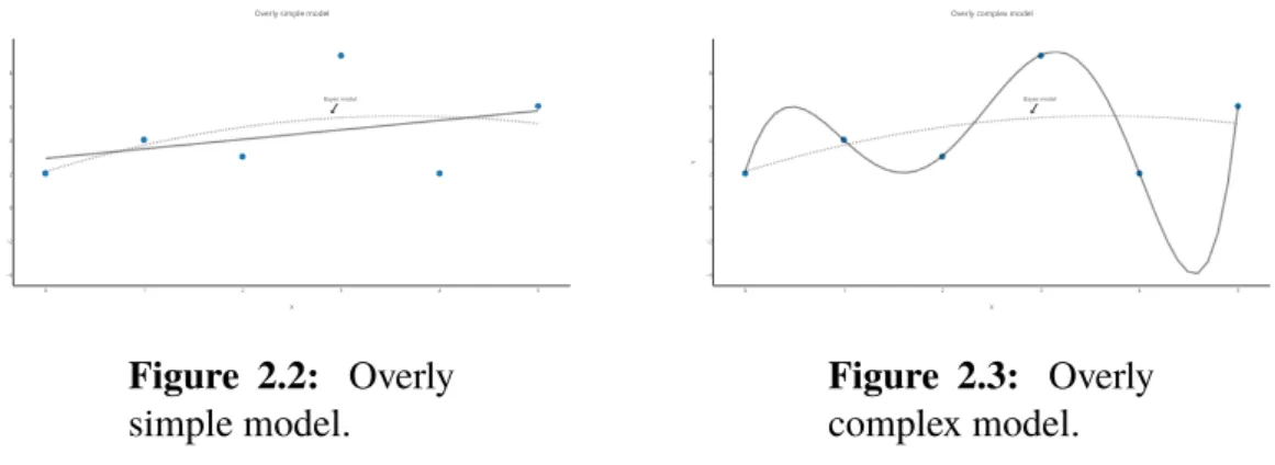
always be an error due to the fact that the model is too simple to cover all instances of the training set. This lack of complexity of the model is called bias(Domingos, 2000). To illustrate, the regression problem described in Figure 2.2 shows that an overly simple model will inevitably fail to account for small variations in the training set. A model with high bias will make false assumptions about the data and can cause the learner to miss relevant relations between features and target features. High bias will generally tend to cause underfitting.

Figure 2.2: Overly simple model.

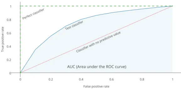
Figure 2.3: Overly complex model.

On the other hand, if a model isoverly complexit might achieve a near perfect match on the training set. However, it will also learn the noise in the training set and will therefore not generalize well on different sets of data. If the model will achieve a perfect match on the training set, it will generally tend to overfit. Even if there is no noise, the model will have errors due to being overly complex. This exaggerated complexity in respect to the complexity of the training set is calledvariance (Domingos, 2000). The analogy in the regression problem can be seen in Figure 2.3. A model with high variance will be overly sensitive to small fluctuations in the training data and can cause modeling of random noise. High variance will generally tend to cause overfitting.

As both bias and variance depend on the complexity of the model, but in opposite di-rection, there must exist a trade-off effect between these sources of error. Due to bias, care must be taken not to use an overly simple model. And vice versa, care must be taken not

2.3 E M

to use an overly complex model with respect to the complexity of the problem due to vari-ance. The bias-variance trade-off applies to all supervised learning such as classification and regression. Apart from the generalization errors produced by bias and variance there is also an unavoidable error that is always present called theirreducible errorcaused by noise in the data.

2.3.5

Visualizing performance trade-offs

Visualizations are often helpful for human comprehension. They also provide a method for comparing machine-learning models side-by-side in a single diagram.

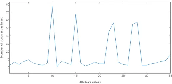
TheROCgraph (Receiver Operating Characteristic) can be used to visualize the trade-off between the detection of true positives and false positives. This can be a good mea-sure of the general efficiency of machine-learning models. The ROC graph is a two-dimensional space that is defined by showing the proportion of true positives (true positive rate) on the vertical axis, and showing the proportion of false positives (false positive rate) on the horizontal axis (see Lantz, 2013, chap. 10).

TheTrue Positive Rate(T P R) is estimated by dividing the number oftruepositives (T P) by the total number of positives (T). T P R is also called hit rate or recall (see Fawcett, 2006, Classifier performance section).

T P R= T P

T P +F N = T P

T .

The False Positive Rate (F P R) is estimated by dividing the number offalse posi-tives (F P) by the total number of negatives (N). F P Ris also calledfall-out orcost(see Fawcett, 2006, Classifier performance section).

F P R= F P

F P +T N = F P

N .

A discreteclassifier model, that outputs a target feature label (as opposed to a prob-abilistic classifier that outputs a probability), will produce a single measure ofT P Rand

F P Rcorresponding to a point in the ROC graph. Depending on where a classifier's cor-responding point is positioned in the graph, some conclusions can be drawn. Classifiers appearing on the left-hand side of the ROC graph, may be considered asconservativeas they will only make positive classifications when there is strong evidence, hence they will generate few false positives. The downside with a conservative classifier is that it will also have a low true positive rate. Classifiers appearing on the upper right-hand side of the ROC graph may inversely be considered asliberalas they will make positive classifi-cations with weak evidence and will classify a high proportion of the positives correctly. However, a liberal classifier will likely also have a high false positive rate. Inductively, a classifier appearing to the northwest of another classifier is better as itsT P Ris higher, itsF P Ris lower or both. See Figure 2.4 depicting the ROC graph. Performance on the left-hand side of the ROC graph is often more interesting as real-world problems are likely dominated by large numbers of negative instances. The point positioned at the uppermost left-hand side of the ROC graph at coordinates(0,1)represents a perfect classifier with perfect performance (see Fawcett, 2006, ROC space section).

Classifiers appearing along the diagonaly=xrepresent models that randomly guesses a target feature. To move away from the diagonal, a classifier must be able to exploit some information in the data. Points positioned in the lower right triangle of the ROC graph will perform worse than random guessing and therefore this region is usually empty. However, if a classifier performs worse than random guessing it will exhibit deterministic behavior and its output can simply be negated to produce a point in the upper left triangle (see Fawcett, 2006, ROC space section).

Figure 2.4: ROC curve and AUC.

A classifier that outputs a probability or a score representing the likeliness that an instance is considered positive is called a probabilistic classifier. Such a classifier can easily be used as a discrete classifier by comparing the output to a threshold. If the output is above the threshold the instance is considered positive. By varying the threshold, a varying degree of the instances in the test set will be classified as positives. It is therefore possible to produce multiple TPR and FPR value pairs on the same classifier model by using multiple threshold values. This can be used to create a ROC curve, by connecting the points produced. A discrete classifier can even be made into a probabilistic one by applyingensemble learningmethods2_{and averaging the results. The ROC curve is useful}

as it can visualize if a model performs better in the conservative or liberal region of the graph. Further it can be revealed at which threshold the classifier has optimal accuracy (the point on the curve that has the smallest distance to the upper left corner has the best accuracy) (Fawcett, 2006).

2_{Ensemble learningis a method for using multiple classifiers concurrently on the same instance to be}

2.4 I

TheAUC(Area Under the ROC Curve) is a statistic that can be used to depict general performance from a ROC curve. It treats the ROC graph as a two-dimensional square and measures the total area under the ROC curve. AUC will range from 0.5 (random guessing) to 1.0 (perfect classifier). There is also a convention using classes similar to academic let-ter grades for inlet-terpreting the AUC scores (see Lantz, 2013, chap. 10).

0.9–1.0 - A (outstanding) 0.8–0.9 - B (excellent/good) 0.7–0.8 - C (acceptable/fair) 0.6–0.7 - D (poor) 0.5–0.6 - F (no discrimination)

2.4

Implementation

Implementing code did inevitable cover a large portion of the algorithm evaluation process. To help reduce the effort put into implementation, existing software and libraries have been used, such as Weka, SciPy, NumPy and Armadillo. Weka is a desktop application that comes packaged with a collection of machine-learning algorithms that can be applied on custom data. SciPy, NumPu, and Armadillo are libraries oriented at statistical, mathematic and scientific computing for Python and C++, respectively.

Some of the algorithms were tested using different implementations, however, as all evaluated algorithms were simple to implement, custom implementations were created in C++ for reasons of flexibility, speed, control, freedom of parallelization, and last but not least --- for fun.

Languages used during implementation: Matlab, R, Python, Java and C++. Most of the data sets used during evaluation were structured as comma-separated-value (CSV) text files.

Chapter 3

Evaluation of Algorithms

The chosen algorithms for this evaluation are: frequent set counting, k-nearest neigh-bors, C4.5, andk-means clustering. These algorithms are all well-known off-the-shelf algorithms with readily available implementations in most programming languages. The first three algorithms are designed to solve classification problems, while the fourth is intended for performing cluster analysis.

The selected algorithms were chosen as they are well documented, easy to understand, and seem fitting for solving the problem at hand. They are also known for having perfor-mance that is competitive with more advanced algorithms, such asNeural networks, given suitable data.

This section contains descriptions of the implementations tested and evaluation mea-sures for each algorithm, respectively. The evaluations were performed using a test ma-chine equipped with a 2.6 GHz quad-core CPU using 8 GB DDR3 SDRAM.

3.1

Data Preparation

Before the algorithms were evaluated, the data needed some preparation. The goal of the preparation was to produce a diverse collection of high quality training sets and test sets for evaluation of the algorithms.

3.1.1

Labeling

All training sets used to train the classifiers need a way of distinguishing between desirable and undesirable outcomes. In order to define a notion of positiveness and negativeness among the instances in a training set, a distinction was made between customers and non-customers. The purpose of this distinction is to be able to train a classifier to identify all customers in a set of data. Hence, the notion of a positive instance was related to customers, and the notion of a negative instance was related to non-customers.

As the company database stores information about existing customers for individual records, it is possible to label all instances in a training set as positive, or negative, depend-ing on the customer states of the instances, respectively. Hence, an additional attribute was added to all training sets and test sets, containing the value “positive” or “negative” which denotes each instance as either a customer, or a non-customer.

3.1.2 Continuous attributes

Continuous attributes contain numeric values which potentially range from negative infin-ity to positive infininfin-ity. This presents a problem as the number of attribute values that need to be accounted for by the models is possibly infinite, and most machine-learning models require a small number of attribute values (Chmielewski and Grzymala-Busse, 1996).

Another problem with attributes containing continuous ranges of values is that it is hard to make generalizations about the values, as many models generalize using equality. For example, given a range of numbers 1–100,000, it can be reasoned that the numbers 5,000 and 5,001 are similar, but to a machine-learning model using symbolic equality as the measure of similarity, this is not true. To the model, the numbers 5,000 and 5,001 are equally dissimilar as 1 and 100,000. In order for the model to be able to make gener-alization about the data, the range of numbers would need to be partitioned into discrete intervals: {[a1, b1], [a2, b2], . . . , [an, bn]}, where bi −ai >= 1, andi = 1, 2, . . . , n.

This process of partitioning continuous ranges into discrete values is calleddiscretization. In this project, two different methods for discretization was evaluated. The first method:

entropy-based partitioning, is part of the C4.5. decision tree algorithm, as an extension, and the second method was invented during the course of this project as an improvement over the first method.

Entropy-based partitioningworks by partitioning the range of continuous values in two partitions, by splitting the sorted range at a threshold value. The threshold value is found by performing an exhaustive search for the maximum gain score over the at-tribute values (gain is a measure of gained information, as described in section 3.4.1). In other words, the maximum threshold is found by iterating over the set of sorted values:

{v1, v2, . . . , vn}, usingvias the threshold in theith iteration, and computing the summed

gain for the the two partitions{v1, v2, . . . , vi}and{vi+1, vi+2, . . . , vn}. The threshold

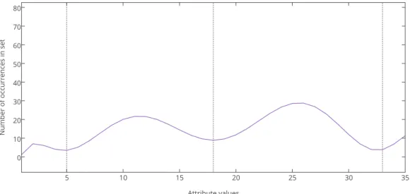
that maximizes the summed gain values of the partitions is chosen as the final value. The improved discretization method analyses the distribution of attribute values, and tries to identify multiple partitions of attribute values that are frequently occurring in the set. The method works by first iterating over all attribute values and counting individual occurrences, creating a distribution of values. As depicted in Figure 3.1, the attribute value distribution will form a jagged curve (most likely). The local maxima of the curve represent the most frequently occurring attribute values, which a classifier should be able to generalize from. Whene.g., two local maxima of near equal value happen to be located far from each other, it becomes hard to create a well-performing discretization by using a binary split, as only one of the maxima will be included. It would be better if the continuous range could be partitioned into multiple parts somehow.

3.1 D P

Figure 3.1: The distribution of attribute values among existing customers.

Our method partitions the distribution by first approximating a polynomial fit on the distribution curve using Least squares (Legendre, 1805), then forms new segments by splitting the distribution at the approximation's minima. Figure 3.2 shows the Least squares approximation of the distribution and Figure 3.3 shows the new segments, partitioned at the approximation's minima. The number of segments created by the approximation fit can be controlled by varying the degree of the polynomial fit.

Figure 3.2: The Least squares approximation for the distribution.

Next, if the new bell-shaped segments are treated as normal distributions, it is possi-ble to compute the expected valuesµi and the standard deviations σi for the individual

intervals of size2σi around the expected values of the individual bell-curve segments:

{[µ1 −σ1, µ1 +σ1], [µ2−σ2, µ2+σ2], . . . , [µn−σn, µn+σn]},

wheren i the number of segments created from the approximation. Finally, all values in the continuous range are partitioned into two groups: therepresentative rangeconsisting of the values that lie within any of the intervals created from the approximation-curve segments, and thenon-representative rangeconsisting of the rest of the values.

Figure 3.3:Four segments are created by splitting the distribution at the approximation's local minima. The dotted lines mark the split points.

The second method was tested to perform marginally better than Entropy-based par-titioning, when used in combination with all three classifier algorithms evaluated in this project. Additionally, the second method was much faster, generally completing the dis-cretization process in seconds, compared to many minutes using Entropy-based partition-ing, which is computationally expensive due to the amount of iterations needed for its exhaustive search for maximum gain.

3.2 Frequent Set Counting using Apriori

Frequent Set Counting (FSC) is often used as an unsupervised learning method for finding frequently occurring subsets of values in a data set (Orlando et al., 2001). The method is similar to n-gram extraction used in natural language processing. n-gram extraction works by counting the frequency ofnconsecutive words in a corpus1_{for determining the}

statistical probability of a specific order ofnwords (see Nugues, 2010, chap. 4). The same principle can be applied on data sets with unordered and unrelated attribute values. All possible combinations of n attribute values are created using every available pair in the

3.2 F S C  A

data,i.e., thepower set2 _{is created, and then all corresponding occurrences are counted.}

By applying FSC on labeled data, the method can be used for supervised learning by counting frequently occurringn-itemsets(ann-itemset consists of n attribute values or

items) that are labeled as positive. Consequently, n-itemsets with a high probability of representing a positive instance can be identified and used to classify unlabeled data.

By varying the size ofn, the complexity of the model can be increased or decreased. Using a smallnwill yield a model withhigh biasandlow variance. Conversely, a largen

will yield a model with low bias and high variance, however, finding frequent occurrences of largen-itemsets will become increasingly difficult as the size ofnincreases.

When the method is applied for classification, athresholdcan be used for determining the minimum number of occurrences of ann-itemset that is needed for it to be used for positive classification. In other words, ann-itemset needs to be sufficiently frequent for it to be representative of the set of data labeled as positive. It is even possible to use combi-nations of frequently occurringn-itemsets that have different sizes ofnfor classification.

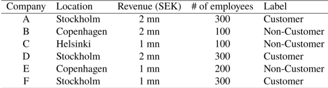
Company Location Revenue (SEK) # of employees Label A Stockholm 2 mn 300 Customer B Copenhagen 2 mn 100 Non-Customer C Helsinki 1 mn 100 Non-Customer D Stockholm 2 mn 300 Customer E Copenhagen 1 mn 200 Non-Customer F Stockholm 1 mn 300 Customer

Table 3.1:Training set of labeled companies.

Table 3.1 shows a training set of companies that are labeled as customers or non-customers of a hypothetical company aspiring to use frequent set counting for identify-ing new customers. Companies labeled as customers are considered as positive instances and companies labeled as non-customers are considered as negative instances. Table 3.2 shows the most frequently occurringn-itemsets among the 3 positive instances. Here, the threshold is set to0.5,i.e., the table only shows then-itemsets present in at least50%of the positive instances. Observe that the2-itemset{Stockholm, 300}is present in all of the positive instances (n = 2as two items are present), as well as the1-itemsets{Stockholm}

and{300}(1-itemsets consist of a single item), which are also present in all instances. The

3-itemset{Stockholm, 2 mn, 300}, the2-itemsets{2 mn, 300}and {Stockholm, 2 mn}

and the1-itemset{2 mn}are present in two thirds of the positive instances.

Using this information it can be hypothesized that companies located in Stockholm which have 300 employees are likely to fit the current customer profile and should therefore be classified as positive instances. Companies located in Stockholm, having 300 employ-ees and that additionally have a revenue of SEK 2 million could also be hypothesized to be positive instances if the threshold is set to a lower value. Note that using the1-itemsets will yield a model with very high bias as, for example, if a classifier would classify all companies located in Stockholm as positive instances, this would likely result in a large number of irrelevant positives (underfitting). On the other hand, using only the biggest 2_{Thepower setof a setSis the set whose members are all possible subsets ofS,e.g., the power set of}

n-itemset n Occurrence {Stockholm, 300} 2 3 of 3 {Stockholm} 1 3 of 3 {300} 1 3 of 3 {Stockholm, 2 mn, 300} 3 2 of 3 {Stockholm, 2 mn} 2 2 of 3 {2 mn, 300} 2 2 of 3 {2 mn} 1 2 of 3

Table 3.2: List of most frequently occurring n-itemsets among companies labeled as customers.

n-itemset available will likely result in very few positive classifications, although most, if not all, will be relevant. Moreover, if the intent is to find new customers then finding the exact same companies labeled as existing customers in the training set is of no use. Therefore it can be concluded that using a too high value fornwill not generalize well to different sets of data and will lead to overfitting.

3.2.1 Implementation

The FSC learner model consists of the process of identifying the frequently occurringn -itemsets and storing these for future classification use. The algorithm used for identifying the frequent itemsets was implemented by first creating asparse matrixrepresentation of all the featuresin the training set. A featureis an attribute-value pair used to describe a value related to an attribute. This is needed as values need to be distinct among the attributese.g., the value “3” will have different meanings when observed within either of the two different attributesemployees orrevenue. The training set depicted in Table 3.1 have 8 distinct features as can bee seen in Table 3.3

Feature # Attribute Value 1 Location Stockholm 2 Location Copenhagen 3 Location Helsinki 4 Revenue 1 mn 5 Revenue 2 mn 6 Employees 100 7 Employees 200 8 Employees 300

Table 3.3:All features present among the positive instances in the training set.

The purpose of using a sparse matrix representation is to get an ordered set of all the features, to save storage space and also to produce a compact representation of the data to utilize locality of reference3 _{for performance gains. The sparse matrix saves storage}

3.2 F S C  A

space as all features can be stored in abinary matrix as opposed to storing the features themselves. An example of a sparse matrix representation can be seen in Table 3.4.

Company Feature 1 Feature 4 Feature 5 Feature 8

A x x x

D x x x

F x x x

Table 3.4: Sparse matrix representation of the positive instances in the training set where “x” indicates that the feature is present. Columns for features 2, 3, 6 and 7 are not displayed as those fea-tures are not present in any of the positive instances.

The next step consists of creating the power set of the set of features by producing su-persetsfrom all the combinations of all features in the training set. Creating the supersets is performed in abottom upmanner,i.e., first,1-itemsets are created from all features, then

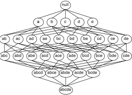
2-itemsets are created from all possible combinations of the1-itemsets, and so on until all combinations ofn-itemsets have been created. However, identifying all itemsets from all combinations of features using a brute force approach will become very expensive both in time and space when the number of features is large (Orlando et al., 2001). The number of supersets that can be generated from a data set containingkdifferent features is2k−1

(Tan et al., 2006). Thus, the search space of itemsets is exponentially large. See Figure 3.4 for a graph depicting all itemsets produced from a data set containing only 5 features.

Figure 3.4: The lattice structure shows the 31 possible itemsets produced from a data set containing 5 features.

To remedy the problem of exponential growth, theApriori principle(Agrawal and Srikant, 1994) can be applied to the problem.

TheAprioriprinciple states:

“If an itemset is frequent, then all of its subsets must also be frequent.” (Tan et al., 2006)

i.e., suppose that the set{b, c, d}is frequent, then all of itssubsets{b, c}, {b, d}, {c, d},

{b},{c}and{d}must also be frequent. Conversely, if a subset{a, b}isinfrequent, then all of itssupersetsmust also be infrequent (Agrawal and Srikant, 1994). Using this strategy, it is possible to immediately prune the entire subtree of supersets that contains the subset

{a, b}, i.e., the subsets {a, b}, {a, b, c}, {a, b, d}, {a, b, e}, {a, b, c, d}, {a, b, c, e}and

{a, b, d, e}can be removed from the search space. By trimming the search space using the Apriori principle, the number of possible itemsets that need to be identified by the algorithm is reduced drastically.

To take advantage of the conclusions drawn above, the frequent set generation can be implemented by using a threshold value indicating the minimum support required for an itemset to continue generating supersets. Starting at the1-itemsets, the frequency of each itemset is counted among all occurrences in the actual data set (e.g., the training set). If the frequency is found to be less than the threshold value, the algorithm will discard the itemset from further use. Take, for example, the set of positive instances represented in the sparse matrix in Table 3.4, if an algorithm were to identify all itemsets using the Apriori principle it would start with counting the frequency of all1-itemsets. Given a threshold value of0.5, a single feature itemset must be present in at least 2 of the 3 instance rows to qualify for further itemset generation. Itemsets{1}, {5}and{8}is present in at least 2 instances, but itemset{4}is only present in 1 instance, hence it is removed from further use. Next, 2-itemsets are created by merging the available1-itemsets resulting in the itemsets

{1, 5},{1, 8}and{5, 8}, of which all are present in 2 or more instances. Finally, a3-itemset

{1, 5, 8}can be created by merging the frequent2-itemsets. The3-itemset itself is present in 2 instances and will thus also qualify as frequent. No more itemsets can be identified as the full search space has been explored. When comparing these results with the frequently occurring itemsets in Table 3.2, it can be seen that the same itemsets have been identified (use Table 3.3 to translate feature numbers into features, respectively).

Pseudocode for the FSC algorithm using the Apriori principle, is showed in Algo-rithm 1.

Algorithm 1Frequent set counting using the Apriori principle.

1: procedureFSC(L, t)

2: F1 ← {frequent1-itemsets} 3: k←2

4: whileFk−1 ̸=∅do

5: C←Generate all possiblek-itemsets fromFk−1

6: Fk ←FilterC, keeping only itemsets that are frequent above threshold.

7: k←k+ 1

3.2 F S C  A

3.2.2

Performance evaluation

Our tests show that the model have high accuracy when performing classification using large itemsets. However, identifying larger itemsets during training requires using a low threshold value, resulting in increased running time. Measured running time for varying threshold values is showed in Table 3.5. As can be seen by the figures, the running time seems to be inversely exponential in relation to the threshold value. The relation between running time and threshold value is also depicted in Figure 3.5.

Threshold Running time (s) Max set size

0.85 1 2 0.8 1 4 0.77 2 6 0.76 7 6 0.75 35 7 0.74 202 7

Table 3.5: Time spent training for varying threshold values.

The size of the itemsets identified during training is also related to the choice of thresh-old value, as can be seen by our measures showed in Table 3.5. Using lower threshthresh-old values will enable the model to identify larger frequent itemsets, but at the cost of longer running times. Thus, it becomes impractical to identify itemsets consisting of more than approximately 7 items, as it simply will take too long.

Figure 3.5: Time spent training for varying threshold values.

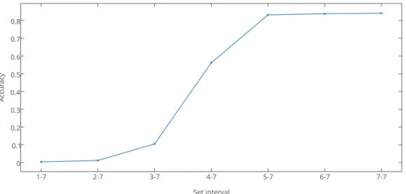
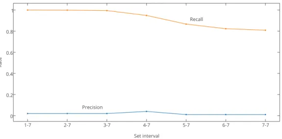
During classification, different intervals of itemset sizes can be chosen for different performance results. By using a broader range of itemset sizes, a higher bias is achieved. For example, using an interval of 1 to 7 means that all itemsets with sizes 1 through 7 are used for classification. Performance results are showed in Table 3.6. The tests was per-formed using a threshold value of 0.75. The results show that higher accuracy is achieved

when using only larger itemset sizes (see Figure 3.6). This however, comes at the cost of reduced recall scores. Also, the precision score is constantly low for all set intervals, never exceeding 0.01 (see Figure 3.7).

Set interval Accuracy Precision Recall F-measure 1–7 0.004 0.002 1.000 0.004 2–7 0.012 0.002 0.999 0.004 3–7 0.105 0.002 0.995 0.004 4–7 0.562 0.004 0.949 0.008 5–7 0.832 0.010 0.867 0.019 6–7 0.838 0.010 0.823 0.019 7–7 0.841 0.010 0.809 0.019

Table 3.6: FSC performance results usingthreshold= 0.75.

Figure 3.6: Accuracy increases as the choice of itemset interval becomes more conservative.

3.3-N N

Figure 3.7: Recall decreases when the set interval is limited to only the larger sizes. Precision is at a constant low.

3.3

k

-Nearest Neighbors

k-nearest neighbors (k-NN) is one of the oldest and simplest algorithms for pattern classi-fication (Cover and Hart, 1967). Despite this it often yields good results in many domains compared to other algorithms. k-NN is considered to be alazy learner, as it delays gen-eralization on the training data until the model is applied for classification (Lantz, 2013). This is opposed to aneager learner, which performs generalization on the data during the training phase. The algorithm usually has good accuracy, but suffers from being compu-tationally expensive both in time and space.

The algorithm works by classifying unlabeled instances by the majority label of itsk -nearest neighbors in the training set. Neighboring instances are determined to be near by means of some distance metric that can be calculated and compared among all instances. See Figure 3.8 for a depiction of a two dimensional k-NN classification model. In the figure, an unlabeled instance is classified by measuring the distances between all labeled instances in the training set, here depicted as black and white dots, and determining the majority vote among thek-nearest instances. For example, ifk = 3, the unlabeled instance will be classified as being associated with the white classas two out of three of the 3-nearest instances are white. A different choice ofk might produce different results,e.g., the unlabeled instance in the figure will belong to theblack classwhenk= 15. Note that using odd numbers forkis preferable when performing binary classification as it avoids a tied vote (see the example in the figure wherek= 8).

When training the model, every instance in the training set is represented by a vector consisting of all the features present in the respective instance. If the vectors carries n

features, respectively, then all vectors are modeled in ann-dimensional space, where the features represent the vector coordinates (see,e.g., Lantz 2013 for a more detailed descrip-tion). The model creates the space of neighboring instances from a labeled training set, and then classifies each unlabeled test-set instance by inserting them one by one into the

Figure 3.8: k-nearest neighbors classification visualized in two dimensions. The big black centerpiece is the unlabeled instance to classify. Black and white dots represent instances with different labels in the training set.

space and finding thek-nearest neighbors, respectively.

The choice ofk is user-defined. Choosing a good value for k is reliant on the char-acteristics of the data. Choosing a smallkmay yield accurate results as closer neighbors will likely be more similar, but it will also cause the learner to be more sensitive to noise in the training data. A largerk will cause the learner to be less dependent on noise, but askapproaches the total number of neighbors in the training set, the result will have less and less predictive value (a majority vote among all instances will be entirely dependent upon the balance of class membership in the training set).

3.3.1 Implementation

There are many different methods for calculating the distance between instances, but it is common to useEuclidean distanceforcontinuous attributes, andHamming distance

orLevenshtein distance(also called edit distance) fordiscrete attributes. These methods are usually good enough, but sometimes the model accuracy can be increased significantly by using more advanced distance metrics (Weinberger and Saul, 2009). TheEuclidean distancebetween two pointsP andQin ann-dimensional space can be calculated using:

3.3-N N

The Hamming distance can be calculated for two strings of equal length by count-ing the number of characters for which the strcount-ings differ (Hammcount-ing, 1950). For example, the Hamming distance between “paper” and “vapor” is 2. For strings of unequal length a generalization of the Hamming distance metric, called theLevenshtein distance(or edit distance), can be used (Levenshtein, 1966). The Levenshtein distance between two strings can be determined as the minimum number of single-character insertions, deletions, or substitutions needed for the strings to become identical. See Algorithm 2 showing pseu-docode for an implementation of a recursive Levenshtein-distance function. A dynamic programmingapproach can be used to avoid the inefficiency of recomputing the distances of the same substrings multiple times.

Algorithm 2Computing Levenshtein distance.

1: procedureLD(s, t)

2: if Length ofsis zerothen ◃Base case: empty strings

3: returnLength oft

4: if Length oftis zerothen ◃Base case: empty stringt

5: returnLength ofs

6: if sandthave same last characterthen 7: cost←0

8: else

9: cost←1

10: returnThe minimum of:

LD(s−1, t)+ 1 ◃Remove last letter froms

LD(s, t−1)+ 1 ◃Remove last letter fromt

LD(s−1, t−1)+cost ◃Remove last letter fromsandt

In this project, all continuous attributes was discretized prior to the model being trained, hence, only the Levenshtein metric was needed (if desired, a lookup table containing type mappings for all attributes in the data can be used to keep the attribute types apart).

3.3.2

Performance evaluation

Tests performed by us show that the k-nearest neighbors algorithm is computationally expensive when applied on large sets of data. Because of the time required, only small fractionsof the training set data could be used for testing. Table 3.7 shows the measured performance of the evaluation implementation on the test machine for varying training set sizes (the number of instances in the training set). The training sets used was balanced using 30% positive instances and 70% negative instances. In this measurement, classifi-cation was performed on the full set of test data containing 2,227,831 unlabeled instances. The data suggests a linear increase in running time as the number of instances in the training set increases. By approximating alinear fiton the data, it is possible to produce a model that can be used for estimating the running time required when using the reference training set in its entirety (it consists of 13,933 labeled instances). This approximation model suggests a running time of approximately 11 hours, which is clearly too much for the existing application (see Figure 3.9 for a linear model of the running time).

# Running time (s) Accuracy Precision Recall F-measure 22 72 0.83 0.01 0.86 0.019 83 241 0.88 0.009 0.54 0.017 167 478 0.90 0.012 0.68 0.024 250 712 0.86 0.012 0.75 0.024 333 946 0.88 0.012 0.75 0.023

Table 3.7: Measured performance results for varying training set sizes. k= 3was used for all measurements.

The results in Table 3.7 show that accuracy is above 80% even for the smallest training set, but the precision is very low at around 1%. This is reflected by the small training set sizes used, as the model have a hard time determining the relevancy of information with such a low amount of training data.

Figure 3.9: Measured running time on the test machine with vary-ing trainvary-ing-set sizes (logarithmic scales used).

When using a smaller test set, however, the full training set could be used for per-formance evaluation. Classification-perper-formance results using this method are showed in Table 3.8. The reference training set used consists of 13,933 labeled instances (30% pos-itive instances), and the test set used contained about 14,000 unlabeled instances. The performance metrics are presented for different values of k. The results show that the model is accurate with both precision and recall reaching almost 90% for small values of

k. The running time using this method was around 4 minutes for all values of k. The graph showed in Figure 3.10 depicts a trend of decreasing accuracy as larger values ofk

3.3-N N

k Accuracy Precision Recall F-measure 3 0.92 0.86 0.88 0.87 5 0.91 0.84 0.85 0.85 9 0.90 0.82 0.83 0.83 15 0.89 0.82 0.82 0.82 19 0.89 0.82 0.81 0.81 25 0.89 0.82 0.80 0.81 33 0.88 0.81 0.80 0.81 45 0.88 0.81 0.79 0.80

Table 3.8:k-nearest neighbors performance results.

Figure 3.10: Measures show that accuracy decreases as k is in-creased.

Figure 3.11 shows that both precision and recall are subject to the same falling trend as larger values ofkare chosen.

Figure 3.11: Both precision (left) and recall (right) decreases as

k is increased (the same horizontal scale as for accuracy is used).

Further, our results show that the bias-variance trade-off can be controlled somewhat by varying the degree of positives in the training set. Training sets with the proportion of instances labeled as positive was varying from 30% to 70% was used for testing and the results can be seen in Figure 3.12.

Figure 3.12: Precision and recall varies as the proportion of pos-itives in the training set is changed.

3.4 D T I  C4.5

Thelearning curveofk-NN (see Figure 3.13) shows that the algorithm has an accu-racy above 80% even when used with smaller training set sizes (as have been previously shown).

Figure 3.13: k-nearest neighbors learning curve.

3.4

Decision Tree Induction using C4.5

Decision tree induction is a machine-learning method used for supervised learning tasks. The method focuses on the modeling of the relationships between inputs and outputs in the form of if-then rules (originally described by Hunt et al. 1966). Decision tree learning is at the top of the list of various classification learning methods for meeting the require-ments of being an off-the-shelf method for data mining. It is quite fast, produces models interpretable to humans, is resistant to irrelevant variables, immune to outliers4_{and can be}

easily extended to be used with many data types such as: discrete classes, numerical and time series (Hastie et al., 2013). Decision tree models often have low bias and high vari-ance and might suffer from bad generalization when used on different sets of data (Geurts, 2002). There are, however, techniques for addressing thise.g., by simplifying the model using discretization, tree pruning and ensemble learning.

Decision tree induction works by creating a tree structure from a labeledtraining set representing the multiple decisions required to reach a leaf of the tree. Each leaf in the tree determine a target-feature or class while the nodes represent attribute based tests with a branch for each possible outcome. The task of the induction is to create a classification model that can decide the class of any instance from its attributes and values (Quinlan, 1986).

Classification of an instance is performed by starting at the root of the tree, evaluating its test and continuing on the branch with the most appropriate outcome. If the selected branch leads to another node, its test is evaluated and the classification algorithm will

continue onto another branch. The process will continue until a leaf has been reached, at which point the instance can be determined to be a member of the class named by the leaf. Table 3.9 shows a training set depicting some weather data over 14 days (Quinlan, 1986). The set has been labeled with the coincidence of a person playing golf or not on that day. By using decision tree induction, it is possible to create a classification model that can be used for determining the likelihood of a person playing golf on any future day, provided that enough weather data is supplied.

Day # Outlook Temperature Humidity Windy Play golf 1 sunny hot high false no 2 sunny hot high true no 3 overcast hot high false yes 4 rain mild high false yes 5 rain cool normal false yes 6 rain cool normal true no 7 overcast cool normal true yes 8 sunny mild high false no 9 sunny cool normal false yes 10 rain mild normal false yes 11 sunny mild normal true yes 12 overcast mild high true yes 13 overcast hot normal false yes 14 rain mild high true no

Table 3.9:A labeled training set with weather data.

An example of a decision tree created from the weather data is showed in Figure 3.14. Notice how the “overcast”-branch is connected directly to a leaf node as all instances in the training set that have the valueovercastfor attributeOutlookhave the labelyes

3.4 D T I  C4.5

Take, for example, a particular Sunday morning, which is not included in the training set, that has the weather characteristics as follows:

Outlook: overcast

Temperature: cool

Humidity: normal

Windy: false

Using the aforementioned decision tree, it can be concluded that the Sunday morning can be classified as a member of the classyes, and is thus a probable candidate day for playing golf.

It is always possible to construct a decision tree that can correctly classify all instances in a training set given that there is enough attribute data available. However, there are usually many such correct decision trees as there is no predetermined order in which the attribute tests should be evaluated. Which attribute should be tested at the root of the tree and which attributes should be tested at the nodes? In the example given in Figure 3.14, the attributeOutlook is tested at the root, but it could just as well be replaced with the attributeHumidityand the tree would look very different. A different tree might perform equally well as a classification rule on the training set, but generally a smaller tree will generalize better to different sets of data as it will suffer less from having high variability being overly complex (Quinlan, 1986).

3.4.1

Implementation

To create a good decision tree during the induction process the algorithmC4.5was used (Quinlan, 1993). C4.5 is an extension to the original algorithm ID3, invented by Ross Quinlan. It provides some improvements over ID3 by being able to handle both con-tinuous and discrete attributes, working with missing attribute values and by providing some built-in pruning capabilities. There is also another extensionC5.0, but it is limited to commercial use and was not explored in this project. The C4.5 algorithm has gener-ally been found to construct simple enough decision trees with good performance, but it can not guarantee that better trees have not been overlooked (Quinlan, 1986). This was, however, not a problem with the particular task of classifying companies as customers, or non-customers, because the models never showed the characteristics of being exces-sively complex. Some of the extensions provided by C4.5 over ID3 was not of interest in this project and was thus not implemented. Also, the discretization extension providing the algorithm the ability to handle continuous numeric attributes was implemented sepa-rately and executed as a separate step in the classification process. This was done, in order to enable evaluation of different types of discretization algorithms, independently of the classifier algorithm.

As C4.5 works in the same way as its predecessor, aside from providing some extended capabilities, the core implementation steps are identical to ID3. The steps of the ID3 algorithm are showed in Algorithm 3 (Quinlan, 1993). Here,Ris the set of attributes to evaluate at the different nodes of the tree andSis the set of instances (the training set). The algorithm works by using a divide-and-conquer strategy for partitioning the set of

Algorithm 3ID3 decision tree induction algorithm.

1: procedureID3(R, S)

2: ifScontains one or more instances, all belonging to the same classthen 3: returnA leaf identifying the class

4: ifSis emptythen

5: returnA leaf identifying the most frequent class in the parent node 6: ifRis emptythen

7: returnA leaf identifying the most frequent class inS

8: A←largestGain(R, S) ◃Get attribute with largest gain inS amongR.

9: {vi |i= 1, 2, . . . , n} ←the values of attributeA.

10: {Si |i= 1, 2, . . . , n} ←the subsets ofS consisting respectively of instances

with valuevi for attributeA.

11: returnA tree with a root node evaluating attributeAand branches labeled

v1, v2, . . . , vngoing respectively to trees:

ID3(R− {A}, S1), ID3(R− {A}, S2), . . . , ID3(R− {A}, Sn)

instances according to the values they contain in respect to the attribute being evaluated. This will continue until all instances in the current subset belong to the same class or until the subset is empty (Quinlan, 1993). The problem is to determine in which order the at-tributes should be evaluated. Our implementation used the standard method of measuring theinformation gained by branching on a particular attribute. Given a probability distri-butionT = {t1, t2, . . . , tm}, the information conveyed by this distribution (also called

theentropyofT) is (Quinlan, 1986):

I(T) =−

m

∑

i=1

(tilog2(ti)).

For example, if T = {0.5, 0.5} then I(T) = 1, if T = {0.8, 0.2}then I(T) = 0.72, and if T = {1, 0}then I(T) = 0(note that a more uniform distribution conveys more information). When performing binary classification, the information needed to identify the class of an instance in the training setSis the information conveyed by the probability distribution of the class affiliations in the set. If pis the number of instances that belong to classPositive, andn is the number of instances that belong to classNegative, then the probability distribution is:

T = { p p+n, n p+n } .

In the case of the weather training set showed in Table 3.9, the information needed to identify the class of an instance isI(T) = I({₁₄9,₁₄5}) = 0.94.

If the training set S is partitioned on the basis of the value of an attribute A, with possible values{a1, a2, . . . , av}, into subsets{S1, S2, . . . , Sv}, thenSiwill contain the

instances inSthat have valueai ofA. The information needed to identify the class of an

instance ofSiisI({_pi+pi_ni, _pin₊i_ni}), wherepiis the number of instances inSithat belong to