A Signal Decomposition Model-Based
Bayesian Framework for ECG Components
Separation
Ebadollah Kheirati Roonizi, and Roberto Sassi, Senior Member, IEEE
Abstract
The paper introduces an improved signal decomposition model-based Bayesian framework (EKS6). While it can be employed for multiple purposes, like denoising and features extraction, it is particularly suited for extracting electrocardiogram (ECG) wave-forms from ECG recordings. In this framework, the ECG is represented as the sum of several components, each describing a specific wave (i.e., P, Q, R, S and T), with a corresponding term in the dynamical model. Characteristic Waveforms (CWs) of the ECG components are taken as hidden state variables, distinctly estimated using a Kalman smoother from sample to sample. Then, CWs can be analyzed separately, accordingly to a specific application. The new dynamical model no longer depends on the amplitude of the Gaussian kernels, so it is capable of separating ECG components even if sudden changes in the CWs appear (e.g., an ectopic beat). Results, obtained on synthetic signals with different levels of noise, showed that the proposed method is indeed more effective in separating the ECG components when compared with another framework recently introduced with the same aims (EKS4). The proposed approach can be used for many applications. In this paper, we verified it for T/QRS ratio calculation. For this purpose, we applied it to 288 signals from the PhysioNet PTB Diagnostic ECG Database. The values of RMSE obtained show that the T/QRS ratio computed on the components extracted from the ECG, corrupted by broadband noise, is closer to the original T/QRS ratio values (RMSE=0.025 for EKS6 and 0.17 for EKS4).
E. Kheirati Roonizi and R. Sassi are with Dipartimento di Informatica, Universit`a degli Studi di Milano, Via Bramante 65, 26013 Crema, Italy (corresponding author, e-mail:[email protected])
Manuscript accepted for publication September 27, 2015.
Copyright (c) 2015 IEEE. Personal use of this material is permitted. However, permission to use this material for any other purposes must be obtained from the IEEE by sending an email to [email protected].
I. INTRODUCTION
The analysis of the electrocardiogram (ECG) is routinely performed to assess cardiac health status. Every ECG beat is composed of different waves, classically labeled as P, Q, R, S and T, which reflect, at the body surface, the electrophysiological activity of the heart. The cardiac cycle begins with the P wave, linked to atrial depolarization, followed by the QRS complex and T wave, which instead corresponds to ventricular depolarization and repolarization. Most of the clinically relevant information can be found within the amplitudes, shapes and intervals between these waveforms. Some examples are ST-waveform analysis for intrapartum fetal monitoring [1], [2], changes in P wave morphology due to various conditions [3], [4], QT interval analysis [5], [6] and T wave alternans (TWA) [7]. So an accurate and robust procedure for automatic ECG labelling is an important goal for clinicians and biomedical engineers. A preliminary ECG components extraction phase, where the different waves are separated from each other, could surely simplify the task.
McSharry et al. proposed an ECG dynamical model (EDM), based on a set of nonlinear state space equations in Cartesian coordinates [8]. Their idea was to construct a dynamical model that repeats the single beat in a pseudo-periodic manner. Subsequently, EDM has been widely used for many applications such as filtering, compression and classification of ECG signals [9], as well as developing an extended Kalman filter (EKF) and extended Kalman smoother (EKS) for noisy ECG filtering [10].
Sameni et al. modified the EDM model by reducing the number of state variables using polar co-ordinates and proposed a Bayesian framework for ECG denoising, also based on EKF and EKS [10]. In the following, these will be referred to as “EKF2” or “EKS2” respectively, since two hidden state variables were used. Thereafter, applications of the modified EDM has been proposed for removing cardiac contaminants [11], generating multi-channels ECG, modeling fetal ECG [12], as well as generating rather realistic synthetic electrocardiogram signals in normal and abnormal conditions [13].
Sayadi et al. introduced a modified EKF structure (“EKF17” as it uses 17 state variables) for ECG denoising and compression [14], as well as for ECG beat segmentation [15]. They also proposed a Gaussian basis function based EDM (“EKF4” and “EKS4”) for robust detection of premature ventricular contractions [16] as well as modeling the temporal dynamics of ECG [17]. Finally, Niknazar et al. have used the EKF structure for fetal ECG extraction using single-channel recordings [18].
Subsequently, a framework for morphological modeling of cardiac signals based on signal decompo-sition, which is capable of generating a realistic synthetic ECG was proposed [19]. Three types of basis functions, including polynomial splines, sinusoidal and Gaussian functions, were alternatively employed to model ECG waves, following the approach of McSharryet al.[8]. However, while the average beat was
represented as a sum of basis functions, it was then repeated in a pseudo-periodic manner to generate multiple subsequent beats. Unfortunately, real ECG signals can be highly non-stationary in practice. So fixing the parameters of a single beat and repeating it to generate multiple beats, is largely an approximation.
In this paper, we aim to improve the morphological model of cardiac signals, described in [19], and to combine it with the Bayesian filtering framework, in order to separate the ECG signal into its component waves, on a beat-to-beat basis. Some very preliminary ideas were presented in [20], and largely extended in here. The rest of the paper is organized as follows. In Section II, the relevant background on EDM and EKF is reviewed. Section III presents the original signal decomposition model-based Bayesian framework for ECG components extraction, comparing it with previous approaches. Applications are presented in Section IV. General remarks and a discussion are given in the final section.
II. BACKGROUND
A. Extended Kalman filter and extended Kalman smoother
The Kalman filter is one of the most widely used methods for estimating the hidden state of a linear dynamical system. In fact, for linear dynamical systems, it is an optimal estimator in the minimum mean square error (MMSE) sense [21]. For nonlinear systems, theextendedKalman filter, which is applied after linearization of the model, might be employed instead. Specifically, let’s consider the undriven non-linear discrete dynamical system
xk+1=f(xk, k) yk=g(xk, k)
and its associated “noisy” system
xk+1=f(xk, wk, k) yk=g(xk, vk, k) , (1)
wherexkis the unobserved underlying state vector, ykis the observation vector at time instant k,f(·)is
the evolution state function, g(·) represents the relationship between the hidden state and observations, wk andvk are process and measurement noise, respectively, with the corresponding covariance matrices
Qk=E{wkwTk} and Rk=E{vkvkT}. The extended Kalman filter for (1) is given as follows [22]:
Time Update: ˆ x−k+1=fk(ˆx+k, w, k)|w=0 Hk−+1=AkHk+ATk +FkQkFkT (2)
Measurement update: ˆ x+k = ˆx−k +Kk h yk−g(ˆx−k, vk, k)|v=0 i Kk=Hk−C T k CkHkCkT +GkRkGTk −1 Hk+=Hk−−KkCkHk− (3) where Ak= ∂f(x,wˆk, k) ∂x x=ˆxk Fk= ∂f(ˆxk, w, k) ∂w w= ˆwk Ck= ∂g(x,vˆk, k) ∂x x=ˆxk Gk= ∂g(ˆxk, v, k) ∂v v=ˆvk (4)
and xˆ−k =E{xk|yk−1,· · ·y1} is a prior estimate of x at time instant k given the previous observations
y1 to yk−1 and xˆ+k =E{xk|yk,· · ·y1} is a posterior estimate that is obtained by correction ofxˆ+k after
observing yk. The matrices Hk− =E{(xk−xˆ−k)(xk−xˆ−k)T} and H +
k =E{(xk−xˆ+k)(xk−xˆ+k)T} are
also defined as the prior andposterior state covariance matrices.
For smoother results, an extended Kalman smoother is usually employed after EKF. It consists of a forward EKF stage followed by a backward recursive smoothing stage. Since EKS uses information brought by “future” observations, it provides better estimates of the current states and follows the ECG morphology more accurately than EKF in noisy scenarios [17].
B. An ECG model based on sum of Gaussian functions
A single ECG beat can be modeled as a sum of N Gaussian functions with different amplitudes and widths centered at specific points in time:
z= N−1 X i=0 αiexp " −(t−θi) 2 2b2i # , (5)
where αi, bi and θi are the amplitude, scale factor and center of the kernels, respectively. It can be
coupled with a model of the heart rate dynamics, to synthesize multiple ECG beats with arbitrary heart rates [8] ˙ θ=ω z= N−1 X i=0 αiexp " −(θ−θi) 2 2b2i #, (6)
(a) Synthetic ECG time(s) 0 1 2 3 4 5 6 7 8 9 10 Amplitude -0.6 -0.4 -0.2 0 0.2 0.4 0.6 (b) Noisy ECG time (s) 0 1 2 3 4 5 6 7 8 9 10 -0.6 -0.4 -0.2 0 0.2 0.4 Noisy ECG
(c) Mean ECG pattern
Samples 0 50 100 150 200 250 Amplitude -0.5 -0.4 -0.3 -0.2 -0.1 0 0.1 0.2 0.3 0.4 0.5 SD Mean
(d) QRS extraction provided by EKS4
time (s) 0 1 2 3 4 5 6 7 8 9 10 Amplitude -0.6 -0.4 -0.2 0 0.2 0.4 Noisy ECG QRS detection
(e) T wave extraction provided by EKS4
time(s) 0 1 2 3 4 5 6 7 8 9 10 -0.6 -0.4 -0.2 0 0.2 0.4 Noisy ECG T-wave detection
(f) QRS extraction provided by EKS6
time (s) 0 1 2 3 4 5 6 7 8 9 10 Amplitude -0.8 -0.6 -0.4 -0.2 0 0.2 0.4 0.6 Noisy ECG QRS detection
(g) T wave extraction provided by EKS6
time(s) 0 1 2 3 4 5 6 7 8 9 10 -0.8 -0.6 -0.4 -0.2 0 0.2 0.4 0.6 Noisy ECG T-wave detection
Fig. 1. QRS complex and T-wave estimates provided by EKS6 and EKS4, when applied to a synthetic signal corrupted by noise with SNR = 18 dB.
where θ is the cardiac phase signal (periodical with a base period defined between −π and π) and ω is the angular speed of thephase signal defined in [12]. A common approach [8] to obtain a dynamical model for z is to differentiate directly (6) to get
˙ θ=ω ˙ z=− N−1 X i=0 αiω θ−θi b2i exp " −(θ−θi) 2 2b2i #. (7)
The EDM in (7) was used in a Bayesian framework with two hidden state variables [10], thus termed EKS2. It can estimate the cardiac phase and ECG amplitude, since they are just assumed as hidden state variables.
Another approach which is more suitable when applying the model to filtering arrhythmias, is to consider different events of the ECG separately as hidden state variables. This idea has been proposed by Sayadi et al. for generating synthetic ECG as well as separate ECG characteristic waveforms (CWs)
[16], [17]. Seven Gaussian kernels were employed to model ECG beats, corresponding to each of the ECG components (P wave, QRS complex, and T wave), and for modeling asymmetries two Gaussian kernels were used for P or T waves (indicated by+ and− superscripts), leading to:
˙ θ=ω ˙ P =− X i∈{P−,P+} αiω θ−θi b2i exp " −(θ−θi) 2 2b2i # ˙ QRS=− X i∈{Q, R, S} αiω θ−θi b2i exp " −(θ−θi) 2 2b2i # ˙ T =− X i∈{T−,T+} αiω θ−θi b2 i exp " −(θ−θi) 2 2b2 i # z=P+QRS+T , (8)
While the kernels are seven, the number of state variables is four, thus the method was termed EKS4. The parameters αi, bi, and θi are identified before applying the Kalman filter. To this aim, after QRS
complex detection, an ECG waveform template is obtained by averaging the time-warped beats [10] and then used to fit the parameters by nonlinear least square estimation. However, morphological changes in abnormal ECG beats or artifacts, which are included when computing the average ECG beat, influence the value of the parameters. This is particularly true for the amplitudesαi. Although they are considered
as a noise process in EKS4, their changes can dramatically impact on filter output, since they appear in the time update (8). To further clarify the issue and to highlight the reasons which motivated our work, the synthetic ECG in Fig. 1(a) displays an episode of alternation of T-wave forms (macroscopic T-wave alternans, TWA). It was inspired by figure 2 in [23]. Such alterations often precede torsade de pointes and sudden cardiac death and their detection is clearly relevant. During the episode depicted in Fig. 1(a) or its noisy version in Fig. 1(b), the T wave amplitude changes in time. The different polarity affects the value of the average template in Fig. 1(c), which is obtained by averaging the noisy signal in Fig. 1(b). The CWs obtained with EKS4 are shown in Fig. 1(d) and 1(e). Unfortunately, the low amplitude of the T waves detected is evident. Morphological changes, especially in abnormal ECG sequences, lead to large errors on the updating state variables and low accuracy on the corresponding ECG component separation. For this reason, in section III we will introduce a new EDM, which no longer depends on the amplitude of the Gaussian kernels, to be used with EKS.
C. Signal modelling using basis functions
Kheirati Roonizi and Sameni [19] worked on the different, but related, problem of morphological modelling of a single ECG beat, through its projection over a set of basis functions. In fact, a single
(a) ECG record08378m. Samples ×104 0.98 1 1.02 1.04 1.06 1.08 1.1 1.12 1.14 1.16 1.18 1.2 Amplitude -2 -1 0 1 2 3 4 record 8378
(b) QRS extraction provided by EKS4
Samples ×104 0.98 1 1.02 1.04 1.06 1.08 1.1 1.12 1.14 1.16 1.18 1.2 Amplitude -2 -1 0 1 2 3 4 EKS4 Original ECG QRS detection
(c) T wave extraction provided by EKS4
Samples ×104 0.98 1 1.02 1.04 1.06 1.08 1.1 1.12 1.14 1.16 1.18 1.2 -2 -1 0 1 2 3 4 EKS4 Original ECG T detection
(d) QRS extraction provided by EKS6
Samples ×104 0.98 1 1.02 1.04 1.06 1.08 1.1 1.12 1.14 1.16 1.18 1.2 Amplitude -1.5 -1 -0.5 0 0.5 1 1.5 2 2.5 3 EKS6 Original ECG QRS detection
(e) T wave extraction provided by EKS6
Samples ×104 0.98 1 1.02 1.04 1.06 1.08 1.1 1.12 1.14 1.16 1.18 1.2 -1.5 -1 -0.5 0 0.5 1 1.5 2 2.5 3 EKS6 Original ECG T detection
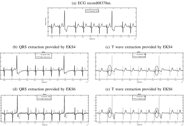
Fig. 2. QRS complex and T-wave estimates provided by EKS6 and EKS4, for record 08378m from the MIT-BIH Atrial Fibrilation Database (afdb).
ECG beat can be represented as the linear combination:
z=
N−1
X
i=0
αiφi(θ), (9)
where{φi}Ni=0−1 is a set of functions used for signal expansion, αi are the expansion coefficients andθis,
as before, the cardiac phase which is defined between−πandπ. Their interest was mainly rooted in signal modelling, not in differentiating CWs, as in the present work. However, some signals, like ECG, admit a decomposition into “natural” components, with a clear physiological meaning (e.g., the well-known P, QRS, and T waves for ECG). If each of theφi components, in the model (9), or their combination, are
meant to describe one of these “natural” subparts of the signal, then the interpretation is straightforward. Gaussian kernels are good candidates for describing each of the ECG component waveforms (even if not orthogonal, the Gaussian expansions is very efficient for describing bumpy waves, e.g., P, QRS and T waves), as the works of the previous section implied. Therefor, putting (5) and (6) in the context of [19],
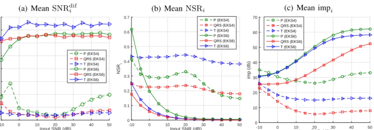
(a) MeanSNRdif i -10 0 10 20 30 40 50 SNR dif i (dB) 15 20 25 30 35 40 45 50 55 Input SNR (dB) P (EKS4) QRS (EKS4) T (EKS4) P (EKS6) QRS (EKS6) T (EKS6) (b) MeanNSRi -10 0 10 20 30 40 50 NSR i 0 0.1 0.2 0.3 0.4 0.5 0.6 0.7 Input SNR (dB) P (EKS4) QRS (EKS4) T (EKS4) P (EKS6) QRS (EKS6) T (EKS6) (c) Mean impi -10 0 10 20 30 40 50 imp (db) 0 10 20 30 40 50 60 70 Input SNR (dB) P (EKS4) QRS (EKS4) T (EKS4) P (EKS6) QRS (EKS6) T (EKS6)
Fig. 3. Mean values ofSNRdifi , NSRi and impi for ECG components estimated by EKS6 and EKS4, as a function of the power of the broadband noise corrupting the input signal.
we now have ˙ θ=ω φi= exp " −(θ−θi) 2 2b2 i # z= N−1 X i=0 αiφi . (10)
Taking the derivative of the basis functionφi, instead of the signalz, they derived the following dynamical
model ˙ θ=ω ˙ φi =−ω θ−θi b2 i ! φi z= N−1 X i=0 αiφi , (11)
which was used to generate synthetic ECG signals.
III. METHODOLOGY
As described before, generating multiple ECG beats using (11) is largely an approximation, due to the non-stationary nature of the ECG. For example, it is known that the QT-interval changes significantly under varying heart rates [5]. Our objective is to estimate the states of a model derived from a modification of (11) using the Bayesian filtering framework described in section II-A. While improving the approach described in section II-B, we will target our goal of separating the ECG components, on a beat-to-beat basis, for further analysis and easier feature extraction.
A. Signal decomposition model-based Bayesian framework
In a preliminary attempt to remove the EDM dependency on CWs amplitude [20], we combined the Bayesian filtering framework with (11) to estimate ECG components. However, in (11), the observation equation still depends on αi.
We move here a step further by defining φei ≡αiexp[−(θ−θi)2/(2b2i)]. A new model can be derived as follows ˙ θ=ω e φi=αiexp " −(θ−θi) 2 2b2i # z= N−1 X i=0 e φi .
Comparing it with (10), the amplitudes now pertain to the basis functions and φei correctly model the ECG components, not just the state as in [20]. In the following, for simplifying the notation, we will drop the tilde and we will simply refer to the new basis functions as φi.
Taking again the derivative of φi, instead of the signalz, the EDM becomes
˙ θ=ω ˙ φi =−αiω θ−θi b2 i ! exp " −(θ−θi) 2 2b2 i # z= N−1 X i=0 φi , (12)
which, in our notation, is similar to the model (8) that is used in EKS4. Nonlinearity is decreased significantly by substituting αiexp[−(θ−θi)2/(2b2i)] with φi in the second equation. Our final EDM
model, which is capable of generating continuous ECG waveforms, is thus as follows ˙ θ=ω ˙ φi =−ω θ−θi b2i ! φi z= N−1 X i=0 φi . (13)
It no longer depends on αi, which are absorbed completely into the state φi.
B. Discretization and implementation
While in the previous section a continuous formulation was used for the ECG dynamical model (as it is more convenient for analytical manipulations), in practical applications a discretized version is needed for EKS. The modified EKS is defined by process and observation equations:
Process equation: θk+1 = (θk+ω∆) mod 2π φi,k+1 = 1−ω∆ θk−θi b2i ! φi,k +ηi,k (14)
where θk and φi,k, i ∈ {P, Q, R, S, T} are state variables, ηi,k are i.i.d. Gaussian random variables
considered to be random additive noise and∆is the sampling interval. At each time stepk, the proposed discrete ECG model consists of six state variables (one for each of P, Q, R, S and T components), plus the cardiac phase θk. To have a more accurate representation, the number of Gaussian basis functions
could be increased, at the cost of an increased complexity of the overall scheme and the risk of modelling noise (see section V for a discussion on the issue). Whenηi,k goes to zero in (14), the time evolution of
each state variable, linked to an ECG waveform, is described by a Gaussian basis functions. However, in any other situation, the new formulation of the EDM is not strictly based on Gaussian kernels, like EKS4 was. Observation equation: ψk=θk+v1,k sk= X i∈{P,Q,R,S,T} φi,k+v2,k , (15)
where sk is the noisy observation (the real ECG) and ψk is the noisy cardiac phase at time instant k.
v1,k andv2,k are zero mean random variables considered to be observation noise. As a result, the state
variables vector, xk, the observation vector, yk, the process noise vector, wk, and the observation noise
vector, vk, are defined as follows:
xk= [θk, φP,k, . . . , φT ,k]
yk= [ψk, sk]
wk= [bP, . . . , bT, θP, . . . , θT, ηP, . . . , ηT, ω]
vk= [v1,k, v2,k]
.
Putting (14) and (15) together, our non-linear discrete dynamical system is as follows: θk+1= (θk+ω∆) mod 2π φi,k+1= 1−ω∆ θk−θi b2 i ! φi,k+ηi,k ψk=θk+v1,k sk= X i∈{P,Q,R,S,T} φi,k +v2,k , (16)
The dynamical model in (16) is still nonlinear. However, the nonlinearity is largely reduced with respect to (8), and it is limited to the productθkφi,k. To linearize it, and then build the EKS, we first reformulate
it into the terminology of (1): θk+1 =f1(θk, ω, k)
φi,k+1 =fi(θk, φi,k, ω, bi, θi, ηi,k, k)
ψk =g1(θk, k) sk =g2(θk, φi,k, k) . Then, following (4): ∂f1 ∂θk = 1 ∂fi ∂θk = −ω∆ b2 i φi,k ∂f1 ∂φi,k = 0 ∂fi ∂φi,k = 1−ω∆θk−θi b2 i ! ∂f1 ∂bi = 0 ∂fi ∂bi = 2ω∆(θk−θi) b3 i φi,k ∂f1 ∂θi = 0 ∂fi ∂θi = ω∆ b2 i φi,k ∂f1 ∂ηi,k = 0 ∂fi ∂ηi,k = 1 ∂f1 ∂ω = ∆ ∂fi ∂ω = −∆(θk−θi) b2 i φi,k ∂g1 ∂θk = 1 ∂g1 ∂φi,k = 0 ∂g2 ∂θk = 0 ∂g2 ∂φi,k = 1 ∂g1 ∂v1,k = 1 ∂g1 ∂v2,k = 0 ∂g2 ∂v1,k = 0 ∂g2 ∂v2,k = 1
so that the matrices Ak, Fk, Ck and Gk are obtained as follows: Ak= 1 O1×5 γ5×1 M5×5 6×6 Fk= O1×5 O1×5 O1×5 ∆ Γ5×5 Λ5×5 I5×5 β5×1 6×16 Ck= 1 O1×5 0 11×5 2×6 Gk=I2×2 , where γ5×1 = " −ω∆ b2 i φi,k #T M5×5 = diag " 1−ω∆θk−θi b2i # Γ5×5 = diag " 2ω∆(θk−θi) b3i φi,k # Λ5×5 = diag " ω∆ b2 i φi,k # β5×1 = " −∆(θk−θi) b2i φi,k #
andI,Oare identity and zero matrices, respectively. In the new formulation of the ECG dynamical model proposed herein, the state matrix Ak is not anymore a constant diagonal matrix, as it was for EKS4, and
it changes at each step k. The non-constant nature of Ak let the overall EKS scheme (which we will
refer to as “EKS6” in the following, as the state is six-dimensional) to be more capable of adapting to changes in amplitude in the ECG waveforms. We will return on this issue, in particular with respect to the comparison with EKS4, in the discussion section.
After linearization, the state variables are propagated in time using equations (2) and (3). This is equivalent to having a set of basis functions updated over time, such that they are distinctly estimated from sample to sample. Therefore ECG components can be extracted even in noisy scenarios, leading to a higher accuracy of the fitting of the model.
IV. APPLICATIONS
The EKS6-based decomposition can find various applications in ECG processing, such as ECG com-ponents extraction,e.g., for T/QRS ratio calculation, denoising or QT interval measurement. As proof of
(a) time (sec) 0.4 0.6 0.8 1 1.2 1.4 1.6 1.8 2 2.2 Amplitude (mV) -1 -0.5 0 0.5 1 1.5 Noisy ECG P-wave detection QRS detection T-wave detection (b) time (sec) 0.4 0.6 0.8 1 1.2 1.4 1.6 1.8 2 2.2 Amplitude (mV) -1 -0.5 0 0.5 1 1.5 Noisy ECG Denoised ECG
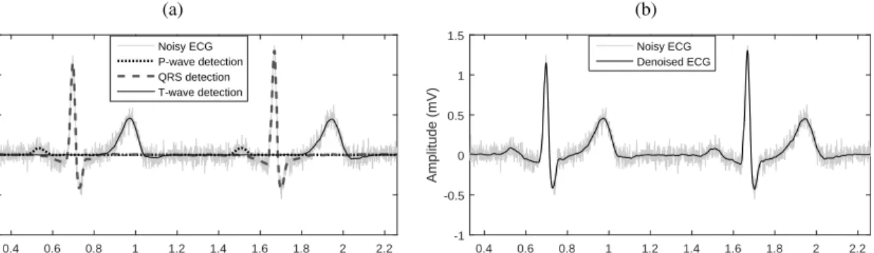
Fig. 4. Panel (a): Noisy ECG beats (SNR = 10 dB) with QRS and T-waves components overlaid, as extracted by means of EKS6. Panel (b): The same noisy ECG overlaid with its de-noised version (the superposition of components produced by EKS6).
concept, we focus on two specific applications.
As a preliminary remark, we clarify that in the following sections, the initial value for the state vector, kernels as well as the covariance matrices of the process and the measurement noise were initialized using the procedure described in [10] and [16]. In particular, using the location of the R-peaks in the signal, an ECG average template waveform,ECG(θ), and its standard deviation,σECG(θ), were obtained
by averaging the time-warped beats. Then, nonlinear least squares was employed (due to the nonlinear dependence) to fit the model
zk=
X
i∈{P,Q,R,S,T}
αiexp[−(θk−θi)2/(2b2i)]
to the ECG template and get the initial values of the parameters of the Gaussian kernels. The angular frequency of the model was set to ω = 2π/hRRi, where hRRi is the average RR-interval of the whole signal and we setθ0 =−π.
The process noise covariance matrixQkwas set to E{wkwkT}=diag(σbp2 , ..., σbT2 , σθp2 , ..., σ2θT, σηp2 , ..., σηT2 , σω2),
where the values were found by computing the magnitude of the amount of deviation of the parameters of φi,k around ECG(θ) to stay within the upper and lower bound of ECG(θ)±σECG(θ) [14], [10].
With respect to the measurement noise covariance matrix R0, E{v21,k} was set to (ω∆)2/12, implying
a uniform error in the location of the R-peak. Then, E{v22,k} was set to the average variance of the perturbation found around baseline (where no P, QRS or T waves are present), across the different beats used to build the template. The measurement noise covariance matrixRk was considered to be diagonal
A. ECG components extraction
1) Preliminary examples: As preliminary example, Fig. 1(f) and 1(g) show the result of applying EKS6 to the synthetic ECG displaying alternation of T-wave forms, as discussed in section II-B. The T wave component follows more precisely, when compared to EKS4 in Fig. 1(d) and 1(e), the ECG morphology, due to the independence of the model from the amplitude.
Furthermore, the decomposition for a specific case (record 08378m from MIT-BIH Atrial Fibrilation Database [24]), using both EKS6 and EKS4, are reported in Fig. 2. EKS4 leads to the distortion of T waves before premature ventricular contractions (PVC), while EKS6 does not, as highlighted using circles in panels (c) and (e). A PVC is a heart beat which is autonomously triggered in the ventricles, and not in the sinus node. PVCs are common events which do not necessarily imply a negative heart condition [25].
2) Synthetic data: For evaluating the performance of the proposed method, we applied it on simulated data, which permit to quantify the decomposition error directly (no gold-standard is available for the decomposition of ECG components of real recordings). Application to real ECG series, will be discussed in the next section.
Single-channel synthetic data were obtained using the EDM on which EKS4 is based and reported in (8). The sampling rate was set to1000Hz, the 250 synthetic series were 20s long and the RR interval durations were allowed a random fluctuation of up to5%in each beat. To make the comparison between EKS6 and EKS4 fair, after applying the former, the Q, R and S waveforms were combined to obtain the QRS complex. Thus, we had three components for each ECG (P wave, QRS complex, and T wave). We produced signals varying the power ofv2,k in (15). The signal-to-noise ratio (SNR) was modulated from
−10 to50 dB.
To simplify the definition of the error metrics, we group together the estimated components into the matrix Φˆ and we call Φthe corresponding matrix of “true” components. Inspired by [18], the estimates
ˆ
Φ are taken to be the linear combination of the true components plus noise v, that is
ˆ Φ =UΦ +Dv, where ˆ Φ = [ ˆφP,φˆQRS,φˆT]T = [ ˆφ1,φˆ2,φˆ3]T Φ = [φP, φQRS, φT]T = [φ1, φ2, φ3]T U = [uij]3×3, i, j= 1,2,3 D= [di]3×1, i= 1,2,3
(a) histogram T/QRS Ratio 0 0.1 0.2 0.3 0.4 Frequency 0 20 40 60 80
(b) with bandpass filter
Original T/QRS Ratio 0 0.1 0.2 0.3 Noisy T/QRS Ratio 0 0.05 0.1 0.15 0.2 0.25 0.3 R2 = 0.928 (c) with EKS6 Original T/QRS Ratio 0 0.1 0.2 0.3 Noisy T/QRS Ratio 0 0.05 0.1 0.15 0.2 0.25 0.3 R2 = 0.969
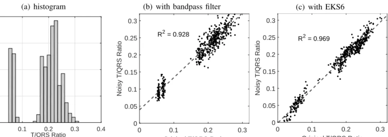
Fig. 5. Panel (a): histogram of T/QRS ratio values for ECG signals from the PhysioNet PTB Diagnostic ECG Database. After contaminating the ECG signal with broadband noise (SNR=10 dB), the T/QRS ratio was recalculated in panel (b) after bandpass (0.5 to 40 Hz) filtering and in panel (c) after EKS6.
and the coefficient matrix U and Dhave to be estimated. Given the fact that the ECG components only minimally overlap in time, we can take their inner product to be approximatively zero. Moreover, ECG components and noise are assumed to be orthogonal. Under these conditions, the estimator Φˆ achieves minimum mean square error (MMSE) if and only if E{( ˆΦ−Φ)TΦˆ} = 0. Hence the MMSE estimates of the matrices of coefficientsU and Dare:
ˆ uij = E{φˆT iφj} E{φT jφj} , ˆ di = E{φˆTiv} E{vTv}.
In a successful component extraction procedure, the interference of undesired components should be minimal, as well as the contribution of noise to the desired component. In other words, in the output of
ˆ
φi, the power ofuˆiiφi (target component) should be much larger than the power of P3j=1,j6=iuˆijφj+ ˆdiv
(other components). That is, in an optimal component separation, the coupling matrixU should be close to the identity matrix andDclose to a null vector. The input signal-to-noise ratio and output signal-to-noise ratio are, respectively, defined as follows:
SNRini = P3 Pφi j=1,j6=iPφj +Pv , SNRouti = uˆ 2 iiPφi P3 j=1,j6=iuˆij2Pφj + ˆd2iPv ,
where Pφ1, Pφ2, Pφ3 and Pv denote powers of P wave, QRS complex, T wave and noise respectively.
SNRini characterizes the problem at hand before performing any separation of components: some compo-nents might be very small with respect to the others and thus difficult to detect. A largeSNRouti indicates
instead that the power of the estimated component φˆi is high against other components and noise. We
further define the improvementSNRdifi = SNRouti −SNRini . A summary of the results of the components extraction procedures on synthetic data is reported in Fig. 3(a).SNRdifi for EKS6 outperformed EKS4.
For evaluating the performance of the proposed method, we also used two other measures of improve-ment. The first one, given by
NSRi= P k φi,k−φˆi,k 2 P kφ2i,k 1/2 ,
is a classical ratio between the power of the reconstruction error and the power of the component φi,k
(a noise-to-signal ratio). The results, reported in Fig. 3(b), show that the reconstruction improvement continues for EKS6 even when the noise corrupting the input signal is small, while it saturates for EKS4. In fact, the results are referred to components separation, not ECG modelling. A wrong component detection or the mixing in the components detected might happen also when little noise is contaminating the input signal. Clearly EKS6 is more tailored to component separation than EKS4, confirming Fig. 3(a). A similar result is conveyed in Fig. 3(c) by the second metrics, inspired by [17]
impi =−10 log10 P k ˆ φi,k−φi,k 2 P k(sk−φi,k)2 (dB), (17)
which instead considers the ratio between the power of the reconstruction error and the power of the other components contained in the original signal sk, defined in (15), including the noise v2,k.
B. T/QRS ratio estimation
Abnormality of ventricular repolarization in the ECG (like ST depression, T wave inversion and QT prolongation) have been shown to be related to cardiovascular mortality. A possible marker of ventricular repolarization is the ratio of T amplitude to QRS amplitude, also known as the T/QRS ratio. The T/QRS ratio has been shown important in distinguishing acute myocardial infraction (AMI) from left ventricular aneurysm (LVA) [26] or very relevant in fetal surveillance [27], [28]. However, the automatic and accurate calculation of this index in noisy scenarios can be very challenging given the possible errors in the location of the fiducial points. EKS6 can improve the estimated T/QRS ratio calculating it from the estimated components, hence reducing the impact of noise.
We tested the approach over the PhysioNet PTB Diagnostic ECG Database [24]. The database contains 549 records from 290 subjects. Each record consists of twelve conventional ECG leads plus the three Frank’s ones, sampled at 1kHz with 16-bit resolution. The feasibility study was limited to 288 ECG segments, of 10s each, obtained from the beginning of selected records (about one for each subject; we considered the twelve standard leads only). The choice was based on the fact that 10s is the standard
duration for diagnostic ECG recordings, where components separation would be of large help (e.g., QT measurement [6]). The T/QRS ratio computation was repeated three times. First, it was performed directly on the original ECG data. Then, white Gaussian noise with a signal-to-noise ratio of 10 dB was added to the ECG signal (“noisy ECG”) and the T/QRS ratio was recomputed. Finally, T-wave and QRS-wave were automatically separated by EKS6, starting from the noisy ECG signal, and the T/QRS ratio was computed a third time employing the amplitudes of the components. In every case, the QRS and T peaks were located as the maximum values in the two windows of length 200ms and 250ms, starting from the Q onset and 100ms after the R-peak, respectively. Beat annotations contained into the database were employed. A Butterworth 3rd order bandpass filter (0.5 to 40 Hz) was employed as preprocessing step when EKS6 was not used. In Fig. 4(a), a couple of noisy ECG beats and the EKS6 outputs are shown. The amplitudes of T and QRS components, as obtained by EKS6, are close to the original ECG. Then, in Fig. 4(b) the ECG, as reconstructed by adding the components, is compared with the original noisy signal. Finally, in Fig. 5, scatter plots of the T/QRS ratios are compared for the original and noisy ECG. When using EKS6, the results are better aligned along a straight line, which indicates that the model rendered the results more resilient to noise.
We also compared EKS6 and EKS4 on this problem. To quantify the performance of the two methods, we employed the root mean square error (RMSE) defined as:
RMSE = 1 n X n Tn QRSn − Tˆn ˆ QRSn !2 1/2 ,
where Tn/QRSn was calculated on the original ECG (nth beat) while Tˆn/QRSˆ n on the components
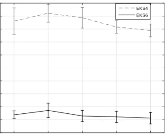
extracted by EKS4 or EKS6, after contaminating the same signal with a broadband noise. The additive Gaussian noise was added with varying SNR (from 0 to 20 dB). The mean and standard deviation (SD) of the RMSE versus different input SNRs achieved over 288 ECG segments (20 repetitions each) are plotted in Fig. 6. A similar approach can be followed for calculating metrics based on other ECG fiducial points, such as the P-wave, PR segment and QT-interval.
V. DISCUSSION AND CONCLUSION
In this paper, a signal decomposition model-based Bayesian filtering method (EKS6) has been in-troduced for ECG signal processing and separation into its components (P, Q, R, S and T waves), by employing an original dynamical model. In the proposed method, the ECG components are directly utilized as hidden state variables, and simultaneously estimated as a time series through an EKS. The simulation results demonstrated that EKS6 has the capability of correctly tracking ECG component waves, on a beat-to-beat basis.
Input SNR (dB) 0 5 10 15 20 RMSE 0 0.02 0.04 0.06 0.08 0.1 0.12 0.14 0.16 0.18 0.2 EKS4 EKS6
Fig. 6. Mean and standard deviation of RMSE in T/QRS ratio values computed from ECG components extracted by means of EKS4 and EKS6, as a function of the broadband noise contaminating the input signal.
There are some theoretical advantages that EKS6 has over other recent works in this context. As compared with EKS2, that uses only two state variables, six state variables are employed, with the advantage of permitting ECG components separation (and not only ECG filtering). Compared to EKS4, it no longer depends on the amplitudes of the Gaussian kernels, so it is able to separate the ECG components, even when abrupt changes happens in the signal. Also, the matrixAkin EKS6 is not constant
in time, hence making it able to better model the nuances in the ECG signal. Finally, EKS linearizes the dynamical system at an operating point by approximating the state model through a first order Taylor series approximation. The truncation of the Taylor series is a poor approximation for most non-linear functions. In fact, the accuracy of the linearization depends on the amount of local nonlinearity in the functions being approximated. Then, the posterior mean and covariance estimations become suboptimal and model errors are introduced. This can lead to instability, particularly when the system dynamics are strongly nonlinear [29]. The EDM proposed here for EKS6 was derived to reduced the nonlinearity of the state model with respect to previous solutions.
From a practical point of view, EKS6 outperformed EKS4 in the tests we performed. For example, components were sometimes mixed up by EKS4 but not by EKS6, as shown for QRS and T waves in Fig. 1 and 2. Surely, EKS6 has two extra state variables with respect to EKS4 (a price to pay for removing amplitude from the model), and, in principle, a larger number of degrees of freedom surely helps EKS6 in better following the ECG components. However, this is not the main source of the performance improvement, but the improvement is due to the new EDM proposed in (13). To support this claim, we increased the number of hidden state variables of EKS4 to six, by using the EDM in (12), which in our
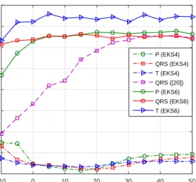
Input SNR (dB) -10 0 10 20 30 40 50 SNR dif (dB)i 15 20 25 30 35 40 45 50 55 P (EKS4) QRS (EKS4) T (EKS4) QRS ([20]) P (EKS6) QRS (EKS6) T (EKS6)
Fig. 7. MeanSNRdifi for ECG components estimated by EKS6 and EKS4. For the latter the number of hidden state variables was increased to six, so that it did not differ from what used in the former. The picture also reports the mean SNRdif
i value obtained when estimating the QRS component using the preliminary EKS described in [20].
notation corresponds to (8). The results are reported in Fig. 7. EKS6 still outperformed the previously suggested solution, even when the number of hidden state variables was made equal. The same figure also contains the partial results (only related to QRS to make the figure easier to read), obtained employing the method described in [20], our preliminary attempt based on (11) and six hidden state variables. Also in this second case, EKS6 displayed better performance. These two further tests support the idea that the improvements derive from the new EDM model itself, possibly underlining the importance of the complete removal of the amplitude dependence. A second technical reason favoring EKS6, might be related to what reported recently by [30], where an EDM, similar to (8), was found to produce a baseline drift in non-invasive fetal ECG, obtained from a similar Bayesian framework.
In the experiments performed in this work, six hidden state variables were employed. The number could be increased to have a more accurate representation of ECG components, at the cost of an increased complexity of the overall scheme. However, this might cause the model to follow undesired observation noises. Information on the measurement and process noises (vk and wk) might help in selecting the
values of the matrixes Qk and Rk, and hence the actual smoothness of the results. The eigenvalues
of Rk−1 should be large when the SNR is high, i.e., little measurement noise vk is assumed, while the
eigenvalue of Q−k1 should be large when the state model is accurate, i.e., wk is supposed to be small
in (1).
ECG components separation through EKS6 is feasible. The same approach is also applicable to robust extraction of other ECG fiducial point markers, including ST-level, QT and PR-intervals. One of the limitation of the present work is the fact that only 10s ECG recordings were considered. The choice was based on the fact this is the standard duration for diagnostic ECG recordings. However, the approach should be tested on longer recordings and we plan to do it in the future. Other immediate future extensions of the present work might be either (i) fetal ECG components separation using non-invasive abdominal ECG recording or (ii) QRST cancellation during atrial fibrillation in adult cardiology for subsequent fibrillatory wave analysis. For example, for fetal ECG components separation, one could modify the parallel EKS introduced in [18] using the new EDM model in (13) for fetal ECG and the one in (7) for maternal ECG.
REFERENCES
[1] K. Ros´en, A. Dagbjartsson, B. Henriksson, H. Lagercrantz, and I. Kjellmer, “The relationship between circulating catecholamines and ST waveform in the fetal lamb electrocardiogram during hypoxia,” Am. J. Obstet. Gynecol., vol. 149, pp. 190–195, 1984.
[2] J. H. Becker, L. Bax, I. Amer-W˚ahlin, K. Ojala, C. Vayssi`ere, M. E. Westerhuis, B.-W. Mol, G. H. Visser, K. Marˇs´al, A. Kwee, and K. G. M. Moons, “ST analysis of the fetal electrocardiogram in intrapartum fetal monitoring: a meta-analysis,”
Obstet. Gynecol., vol. 119, pp. 145–154, 2012.
[3] F. Censi, G. Calcagnini, C. Ricci, R. Ricci, M. Santini, A. Grammatico, and P. Bartolini, “P-wave morphology assessment by a Gaussian functions-based model in atrial fibrillation patients,”IEEE Trans. Biomed. Eng., vol. 54, pp. 663–672, 2007. [4] M. A. Colman, O. V. Aslanidi, J. Stott, V. Holden, and H. Zhang, “Correlation between P-wave morphology and origin of atrial focal tachycardia - insights from realistic models of the human atria and torso,”IEEE Trans. Biomed. Eng., vol. 58, pp. 2952–2955, 2011.
[5] P. Kligfield, K. G. Lax, and P. M. Okin, “QT interval-heart rate relation during exercise in normal men and women: Definition by linear regression analysis,”JACC, vol. 28, pp. 1547–1555, 1996.
[6] M. Malik, P. F¨arbom, V. Batchvarov, K. Hnatkova, and A. J. Camm, “Relation between QT and RR intervals is highly individual among healthy subjects: implications for heart rate correction of the QT interval,”Heart, vol. 87, no. 3, pp. 220–228, 2002.
[7] R. L. Verrier, T. Klingenheben, M. Malik, N. El-Sherif, D. V. Exner, S. H. Hohnloser, T. Ikeda, J. P. Mart´ınez, S. M. Narayan, T. Nieminen, and D. S. Rosenbaum, “Microvolt T-wave alternans: Physiological basis, methods of measurement, and clinical utility-consensus guideline by ISHNE,”J. Am. Coll. Cardiol., vol. 58, pp. 1309–1324, 2011.
[8] P. E. McSharry, G. D. Clifford, L. Tarassenko, and L. A. Smith, “A Dynamic Model for Generating Synthetic Electrocardiogram Signals,”IEEE Trans. Biomed. Eng., vol. 50, pp. 289–294, 2003.
[9] G. D. Clifford, A. Shoeb, P. E. McSharry, and B. A. Janz, “Model-based filtering, compression and classification of the ECG,”Int. J. Bioelectromagn., vol. 7, pp. 158–161, 2005.
[10] R. Sameni, M. B. Shamsollahi, C. Jutten, and G. D. Clifford, “A nonlinear Bayesian filtering framework for ECG denoising,”
IEEE Trans. Biomed. Eng., vol. 54, pp. 2172–2185, 2007.
[11] R. Sameni, M. B. Shamsollahi, and C. Jutten, “Model-based Bayesian filtering of cardiac contaminants from biomedical recordings,”Physiol. Meas., vol. 29, pp. 595–613, 2008.
[12] R. Sameni, G. D. Clifford, C. Jutten, and M. B. Shamsollahi, “Multichannel ECG and noise modeling: Application to maternal and fetal ECG signals,”EURASIP J. Adv. Signal Process., pp. 043 407:1–14, 2007.
[13] G. D. Clifford, S. Nemati, and R. Sameni, “An artificial vector model for generating abnormal electrocardiographic rhythms,”
Physiol. Meas., vol. 31, pp. 595–609, 2010.
[14] O. Sayadi and M. B. Shamsollahi, “ECG denoising and compression using a modified extended Kalman filter structure,”
IEEE Trans. Biomed. Eng., vol. 55, pp. 2240–2248, 2008.
[15] ——, “A model-based Bayesian framework for ECG beat segmentation,”Physiol. Meas., vol. 30, pp. 335–352, 2009. [16] O. Sayadi, M. B. Shamsollahi, and G. D. Clifford, “Robust detection of premature ventricular contractions using a
wave-based Bayesian framework,”IEEE Trans. Biomed. Eng., vol. 57, pp. 353–362, 2010.
[17] ——, “Synthetic ECG generation and Bayesian filtering using a Gaussian wave-based dynamical model,”Physiol. Meas., vol. 31, pp. 1309–1329, 2010.
[18] M. Niknazar, B. Rivet, and C. Jutten, “Fetal ECG extraction by extended state Kalman filtering based on single-channel recordings.”IEEE Trans. Biomed. Eng., vol. 60, pp. 1345–1352, 2013.
[19] E. Kheirati Roonizi and R. Sameni, “Morphological modeling of cardiac signals based on signal decomposition,”Comput.
Biol. Med., vol. 43, pp. 1453–1461, 2013.
[20] E. Kheirati Roonizi and M. Fatemi, “A modified Bayesian filtering framework for ECG beat segmentation,” inProc. of
the 22nd Iranian Conference on Electrical Engineering (ICEE), 2014, pp. 1868–1872.
[21] S. M. Kay,Fundamentals of Statistical Signal Processing: Estimation Theory. Upper Saddle River, NJ, USA: Prentice-Hall, Inc., 1993.
[22] B. D. O. Anderson and J. B. Moore,Optimal Filtering. Dover Publications, Inc., 1979.
[23] E. A. Raeder, D. S. Rosenbaum, R. Bhasin, and R. J. Cohen, “Alternating morphology of the QRST complex preceding sudden death,”N. Engl. J. Med., vol. 326, pp. 271–272, 1992.
[24] A. L. Goldberger, L. A. N. Amaral, L. Glass, J. M. Hausdorff, P. C. Ivanov, R. G. Mark, J. E. Mietus, G. B. Moody, C.-K. Peng, and H. E. Stanley, “Physiobank, Physiotoolkit, and Physionet: Components of a new research resource for complex physiologic signals,”Circulation, vol. 101, pp. e215–e220, 2000.
[25] L. E. Hinkle, S. T. Carver, and D. C. Argyros, “The prognostic significance of ventricular premature contractions in healthy people and in people with coronary heart disease,”Acta Cardiol., vol. Suppl 18, pp. 5–32, 1974.
[26] S. W. Smith, “T/QRS ratio best distinguishes ventricular aneurysm from anterior myocardial infarction,”Am. J. Emerg. Med., vol. 23, pp. 279–287, 2005.
[27] K. G. Ros´en, I. Amer-W˚ahlin, R. Luzietti, and H. Nor´en, “Fetal ECG waveform analysis,”Best Pract. Res. Clin. Obstet.
Gynaecol., vol. 18, pp. 485–514, 2004.
[28] I. Amer-W˚ahlin, S. Arulkumaran, H. Hagberg, K. Marˇs´al, and G. Visser, “Fetal electrocardiogram: ST waveform analysis in intrapartum surveillance,”BJOG, vol. 114, pp. 1191–1193, 2007.
[29] P. Maybeck, Stochastic Models, Estimation, and Control. Mathematics in Science and Engineering. Elsevier Science, 1982.
[30] J. Behar, J. Oster, and G. Clifford, “A Bayesian filtering framework for accurate extracting of the non invasive FECG morphology,” inComputing in Cardiology, vol. 41, 2014, pp. 53–56.
Ebadollah Kheirati RooniziEbadollah Kheirati Roonizi was born in Estahban, Iran, in 1982. He received a B.Sc. in computer engineering and M.Sc. in bioelectrical engineering both from Shiraz University, Iran, in 2006 and 2011, respectively. As a member of Biomedical Image and Signal Processing group, he is currently working toward the Ph.D. degree in computer science at the University of Milan, Crema, Italy. His research interests include signal modeling/processing, especially for cardiac modeling and simulation, ventricular repolarization, functional data analysis. He is working on aspects related to modeling, filtering, separation and analysis of cardiac signal waveforms in his Ph.D. thesis.
Roberto Sassi(M’06SM’12) received the Laurea degree (B.Sc. and M.Sc.) in electronic engineering in 1996, and the Ph.D. degree in biomedical engineering in 2001, both from Politecnico di Milano, Italy. After graduating, he worked as Postdoctoral Researcher at the University of California, Santa Cruz, in mathematical modeling of non-Newtonian fluids and at Politecnico di Milano on ECG signals and atrial fibrillation. He is currently Associate Professor at Universit`a degli Studi di Milano, Italy. He taught courses of digital signal and image processing, statistics and programming. His research interests include biomedical signal processing, linear and nonlinear time series analysis, biometrics, with special emphasis on privacy protection issues, and applied mathematics.