Graph-based Data Modeling and Analysis for Data Fusion in Remote Sensing

(1)

Rochester Institute of Technology Rochester Institute of Technology

RIT Scholar Works

Theses

12-2016

Graph-based Data Modeling and Analysis for Data Fusion in

Remote Sensing

Lei Fan

[email protected]

Follow this and additional works at: https://scholarworks.rit.edu/theses Recommended Citation

Recommended Citation

Fan, Lei, "Graph-based Data Modeling and Analysis for Data Fusion in Remote Sensing" (2016). Thesis. Rochester Institute of Technology. Accessed from

This Dissertation is brought to you for free and open access by RIT Scholar Works. It has been accepted for inclusion in Theses by an authorized administrator of RIT Scholar Works. For more information, please contact

(2)

Graph-based Data Modeling and Analysis for Data Fusion in

Remote Sensing

by

Lei Fan

B.S. Optical Engineering, Nanjing University of Science and Technology, 2011

A dissertation submitted in partial fulfillment of the requirements for the degree of Doctor of Philosophy in the Chester F. Carlson Center for Imaging Science

College of Science

Rochester Institute of Technology December, 2016

Signature of the Author

Accepted by

(3)

CHESTER F. CARLSON CENTER FOR IMAGING SCIENCE COLLEGE OF SCIENCE

ROCHESTER INSTITUTE OF TECHNOLOGY ROCHESTER, NEW YORK

CERTIFICATE OF APPROVAL

Ph.D. DEGREE DISSERTATION

The Ph.D. Degree Dissertation of Lei Fan has been examined and approved by the dissertation committee as satisfactory for the

dissertation required for the Ph.D. degree in Imaging Science

Dr. David Messinger, Dissertation Advisor, Date

Dr. David Ross, External Chair, Date

Dr. Anthony Vodacek, Date

Dr. Sildomar Monteiro, Date

(4)

Graph-based Data Modeling and Analysis for Data Fusion in

Remote Sensing

by Lei Fan Submitted to the

Chester F. Carlson Center for Imaging Science in partial fulfillment of the requirements

for the Doctor of Philosophy Degree at the Rochester Institute of Technology

Abstract

Hyperspectral imaging provides the capability of increased sensitivity and discrimination over traditional imaging methods by combining standard digital imaging with spectro-scopic methods. For each individual pixel in a hyperspectral image (HSI), a continuous spectrum is sampled as the spectral reflectance/radiance signature to facilitate identifica-tion of ground cover and surface material. The abundant spectrum knowledge allows all available information from the data to be mined. The superior qualities within hyperspec-tral imaging allow wide applications such as mineral exploration, agriculture monitoring, and ecological surveillance, etc. The processing of massive high-dimensional HSI datasets is a challenge since many data processing techniques have a computational complexity that grows exponentially with the dimension. Besides, a HSI dataset may contain a lim-ited number of degrees of freedom due to the high correlations between data points and among the spectra. On the other hand, merely taking advantage of the sampled spectrum of individual HSI data point may produce inaccurate results due to the mixed nature of raw HSI data, such as mixed pixels, optical interferences and etc.

Fusion strategies are widely adopted in data processing to achieve better perfor-mance, especially in the field of classification and clustering. There are mainly three types of fusion strategies, namely low-level data fusion, intermediate-level feature fu-sion, and high-level decision fusion. Low-level data fusion combines multi-source data that is expected to be complementary or cooperative. Intermediate-level feature fusion

(5)

4

aims at selection and combination of features to remove redundant information. Decision level fusion exploits a set of classifiers to provide more accurate results. The fusion strate-gies have wide applications including HSI data processing. With the fast development of multiple remote sensing modalities, e.g. Very High Resolution (VHR) optical sensors, Li-DAR, etc., fusion of multi-source data can in principal produce more detailed information than each single source. On the other hand, besides the abundant spectral information contained in HSI data, features such as texture and shape may be employed to represent data points from a spatial perspective. Furthermore, feature fusion also includes the strategy of removing redundant and noisy features in the dataset.

One of the major problems in machine learning and pattern recognition is to develop appropriate representations for complex nonlinear data. In HSI processing, a particular data point is usually described as a vector with coordinates corresponding to the inten-sities measured in the spectral bands. This vector representation permits the application of linear and nonlinear transformations with linear algebra to find an alternative repre-sentation of the data. More generally, HSI is multi-dimensional in nature and the vector representation may lose the contextual correlations. Tensor representation provides a more sophisticated modeling technique and a higher-order generalization to linear sub-space analysis.

In graph theory, data points can be generalized as nodes with connectivities measured from the proximity of a local neighborhood. The graph-based framework efficiently characterizes the relationships among the data and allows for convenient mathematical manipulation in many applications, such as data clustering, feature extraction, feature selection and data alignment. In this thesis, graph-based approaches applied in the field of multi-source feature and data fusion in remote sensing area are explored. We will mainly investigate the fusion of spatial, spectral and LiDAR information with linear and multilinear algebra under graph-based framework for data clustering and classification problems.

(6)

Acknowledgements

Pursuing P.hD. degree in Imaging Science here at R.I.T has become one of the greatest experiences of mine. I enjoyed my talking with every professor and staffhere in Chester F. Carlson Center, and I am truly proud of being one of the Imaging Science family.

My deep gratitude goes first to my advisor Professor David Messinger, who expertly and patiently guided me through my five years study and life in Rochester. His broad knowledge in remote sensing field and enthusiasm for imaging science has always encour-aged me and constantly engencour-aged me with my research. His skillful guidance, innovative ideas and tolerant altitude are greatly appreciated. Apart from being a wonderful aca-demic advisor and program director, Professor David Messinger is also a great life and career mentor to me.

I would like to express my sincere appreciation to my committee members: Dr. Anthony Vodacek, Dr. Sildomar Monteiro, Dr. David Ross and Dr. Tony Harkin. Though Dr. Tony Harkin can no longer serve on my committee due to a health problem, I want to express my gratitude to him for providing insightful advice to my research and I want to send my best wishes to him. I am extremely grateful to all my committee members for being supportive to my proposed work and providing to me brilliant suggestions and comments. Special thanks to Dr. David Ross for agreeing to serve on my thesis committee even when he has not even met me. I am honored to have Dr. David Ross as my external chair during Dr. Tony Harkin’s absence.

I also would like to sincerely thank all the faculty and staffin the Chester F. Carlson Center for their enthusiasm in imaging science and their willingness to offer help in every way. I am grateful to Cindy Schultz, Sue Chan, Marilyn Lockwood and Joyce French for always being willing to help me with all kinds of paperwork and school affairs. A special mention to Cindy Schultz, greatly missed, who always had her door open to me and had always been cheerful to everyone.

Lots of thanks to all my fellow officemates, classmates and friends at R.I.T. I learnt a lot from everyone and enjoyed the five years life with them in Rochester. I also wish to thank the staff, Susan Joseph and Jeffrey Cox, from the International Student Service Center for always providing me great suggestions and offering me prompt help with my visa to work and study in the US. Also, I want to express my great gratitude to my mentors, Alex Loui, Basak Oztan and Elizabeth Edmunds, during my three internships

(7)

6

experiences, respectively. Without their support and guidance, I can never gain such valuable industry experiences and great memories with co-workers.

Above ground, I am indebted to my family in China, whose value to me only grows with time. My deepest gratitude to my parents: Aihua Han and Sixin Fan, for their unconditional love and support at all times. Also, I want to thank my parents in-law: Xiulan Shao and Yuliang Wang, for their encouragement and understanding. And finally, I acknowledge my husband, Xiyu, who is my greatest champion, life companion, my anchor and best friend for the past and for the future. Without them, my thesis would not have been possible.

In the end, I thank all my friends for their supports and encouragements to me all the time. I also would like to extend my thanks to those who has helped me in every aspects in my life.

(8)

To my beloved family and friends

(9)

6.1 Conclusions . . . 142 6.1.1 Topology-based semi-supervised classification . . . 142 6.1.2 Self-tuning spectral clustering . . . 142 6.1.3 Graph-based spatial-spectral fusion with composite kernels . . . . 143 6.1.4 Tensor for pixel/superpixel spatial-spectral HSI classification . . . . 143 6.1.5 Tensor for HSI and LiDAR feature fusion . . . 144 6.2 Limitations and Future Work . . . 144

(12)

List of Figures

2.1 Example of Hyperspectral imaging and LiDAR imaging. . . 27

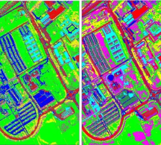
3.1 Classification Maps for (a) Cooke City and (b) Pavia University. . . 50 3.2 Cooke City Classification Map. Left: using TAD+GML; OA=84.5%. Right:

using TAD+MDM; OA=52.5%. . . 50 3.3 Pavia University Classification Map. Left: using TAD+GML; OA=62.9%.

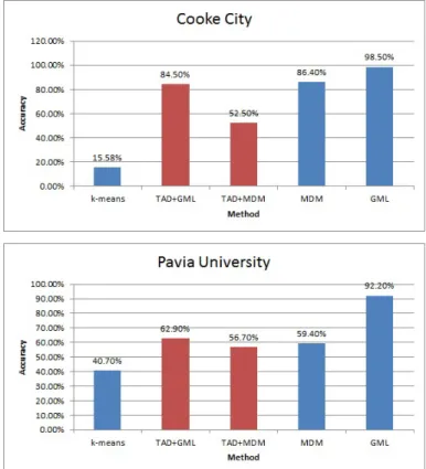
Right: using TAD+MDM; OA=56.7%. . . 50 3.4 Comparison of the OA of traditional unsupervised, supervised classifiers

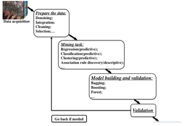
and the semi-supervised classifier presented in this paper. . . 51 4.1 Basic data mining procedures for remote sensing imagery. . . 58 4.2 Three stages in spectral unmixing. . . 59 4.3 5-by-5 neighborhood patch of one pixel and the co-occurrence matrix for

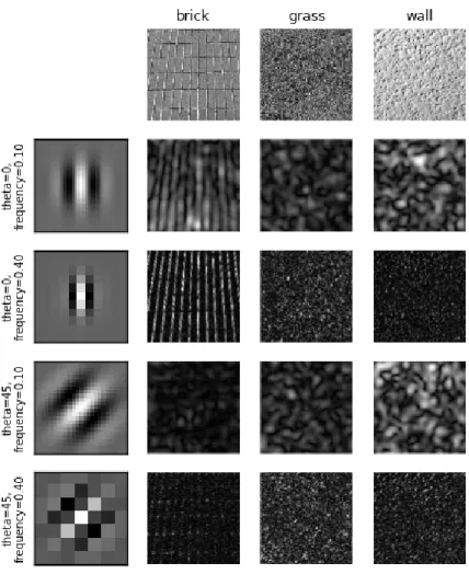
the patch for pixel pair of d=1,θ=0. . . 63 4.4 Three images (brick, grass, wall) with different texture structures filtered

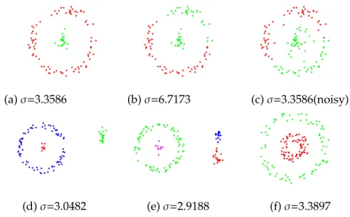
with Gabor filter banks of four different frequency and orientation. Re-trieved fromhttp://scikit-image.org/docs/dev/auto_examples/plot_ gabor.html . . . 65 4.5 1stto 5thorder symmetric neighbors to central pixelX(c) in a MRF model. 66 4.6 The example of LE with fixed scaling parameter σ. Top row: a small

perturbation in the scaling parameterσor in the data points gives rise to very different results. Bottom row: the optimalσfor each data set turned out to be different. . . 71

(13)

LIST OF FIGURES 12

4.7 (a) Input data points. (b) Graph constructed use Gaussian kernel with a uniformσ. (c) Graph constructed use local scale similarity measure. . . 72 4.8 Comparison of graphs constructed via Gaussian kernel for similarity

mea-sure using local tuning parameters. σi for data point xi is defined as its

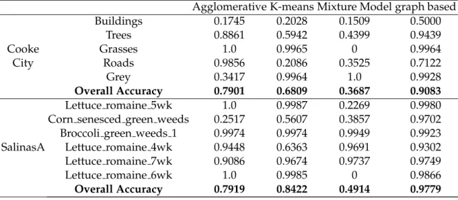
distance to thek_th neighbor. In (b) and (c),kis set to a fixed value for all data points. In (d),kis obtained by adaptivek-nearest neighbor approach. 73 4.9 Results on Ground Truth only of Cooke City and Salinas Scene. . . 76 4.10 Comparison of segmentation results of Agglomerative clustering, K-means

and Gaussian Mixture Model and our graph based splitting and merging. 76 4.11 Flowchart of the proposed spatial-spectral clustering scheme. . . 81 4.12 Left: Graph with two clusters and its affinity matrix. Right: Reinforced

graph with conductivity matrix. . . 81 4.13 Clustering results comparison. Only spectral information is used in the

clustering. . . 83 4.14 Clustering results using our tuning by EAP graph matrices approach and

weighted summation method. Results of using conductivity matrix instead of affinity matrix are also included. . . 84 5.1 A simple illustration of fibers and slices in a third order tensor. Third-order

tensors have column, row, and tube fibers; horizontal, lateral, and frontal slices. . . 88 5.2 Illustration of the mode-nmultiplications of a third-order tensor by a

ma-trix. Mode-1 multiplicationY=X ×₁_U(1)_{. . . .} ₈₉

5.3 Illustration for 3-way Tucker decomposition. 3-order tensorX ∈ _RI1×I2×I3

is decomposed into three basis matrices A(1),A(2),A(3) and a core tensor

G ∈ _RJ1×J2×J3,_J

1 ≤ I1,J2 ≤ I2,J3 ≤ I3. Also, there is a term Gdenotes the

approximation error. . . 91 5.4 A graphical representation of the third-order CP decomposition as a sum

of rank-one tensorsX = PJ

ja1j◦a2j ◦a3j +E.Each vector ai j is a column

vector of the corresponding loading matrix. . . 92 5.5 CP model as a special Tucker decomposition with a super-diagonal core

(14)

LIST OF FIGURES 13

5.6 Left: simultaneous approximate matrix factorizations, given a set of second order tensors Xk ∈ _RI1×I2, ₍_k = ₁,₂...,_K_{). Right: Tucker-2 decomposition}

taken all the second order tensors as a single unified third order tensor

X ∈_RI1×I2×K_{. . . .} ₉₄

5.7 A simple illustration of a typical multilinear subspace learning algorithm workflow. . . 97 5.8 Tensor representation for pixels in a high dimensional image (HSI/EMAP).

Comparison between a conventional vector representation for a pixel and a second order tensorial representation with four spatial neighbors consid-ered. . . 101 5.9 The second order tensorial representations for all pixels in an image cube

are concatenated along the third mode to form a third order tensor. . . 102 5.10 Two types local neighborhood searching: k nearest neighbor searching

(k=4 in the figure) and radius searching (r is the radius in the figure). . . 104 5.11 Simple illustration of some of the LiDAR point cloud local features. . . 107 5.12 A HSI image cube is represented by the concatenation of the 3rdordertensor

representations of all pixels. The spatial, spectral and geometric features for each pixel is represented as a matrix. With local neighborhood information included, a 3rdordertensor is formulated to fuse HSI and LiDAR features. . 109 5.13 Features extracted from a superpixel can be formulated into high order

tensor representation. . . 111 5.14 Workflow of spatial-spectral pixel-wise and superpixel-wise image

classi-fication with 2ndtensor representation for every HSI data point. . . 125 5.15 Left: Pavia University image in RGB. Middle: Training data. Right: Testing

data. . . 126 5.16 Some feature images in EMAPs for Pavia University. . . 127 5.17 Top: Plots of the accuracy for each class in the ROIs for LPP and PCA

applied on original HSI and EMAPs. Bottom: Bar plots for: Left: Average accuracy, Middle: Overall accuracy, Right: Kappa coefficient. . . 128

(15)

LIST OF FIGURES 14

5.18 Top: Plots of the accuracy for each class in the ROIs for TLPP, MPCA and LRTA applied on EMAPs with pixel-wise DR and superpixel-wise DR. Bottom: Bar plots for: Left: Average accuracy, Middle: Overall accuracy, Right: Kappa coefficient. . . 129 5.19 Classification maps of the Pavia University dataset obtained using DR

methods of the following: First row: TLPP; Second row: MPCA; Third row: LRTA. In each row from left to right: pixel-wise classification, superpixel-wise classification of sizeS=6, m=0.01, superpixel-wise classification of sizeS=12, m=0.01. . . 130 5.20 Data sets for HSI and LiDAR fusion: (a) HSI, (b) the LiDAR height map,

(c) training ROI, and (d) validation ROI. . . 132 5.21 Some of the features being extracted after tensor-based dimensionality

reduction. . . 138 5.22 Classification map of the five tensor based dimensionality reduction

(16)

List of Tables

2.1 Parameters of eight Hyperspectral instruments. . . 28

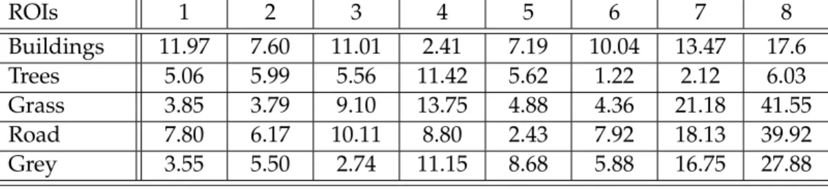
3.1 Bhattacharyya distance between every pair of classes generated using TAD with labeled data. . . 48

4.1 Accuracy of using agglomerative clustering, K-means, gaussian mixture model and our graph based scheme for Cooke City and Salinas-A data sets. 77 4.2 Comparison of class accuracy and overall accuracy of each method. . . 84

4.3 Class accuracy and overall accuracy 1) comparison of using affinity matrix and conductivity with tuning method; 2) comparison of using affinity matrix and conductivity with direct summation method. . . 84

5.1 The training and testing data provided with HSI image . . . 133

5.2 Performance comparison of the two tensor factor analysis algorithms NTF, NTD; the three tensor multilinear subspace learning algorithms TLPP, MPCA, TNPE; and the three traditional linear subspace learning algo-rithms LPP, PCA and NPE. . . 135

5.3 Confusion Matrix - CP . . . 135

5.4 Confusion Matrix - MPCA . . . 136

5.5 Confusion Matrix - NTD . . . 136

5.6 Confusion Matrix - TLPP . . . 136

5.7 Confusion Matrix - TNPE . . . 137

(17)

Chapter 1

Introduction

1.1

Motivation and Background

1.1.1 Multi-modalities of Remotely Sensed Data

Remote sensing is the acquisition and analysis of information from objects without using an instrument to collect the data in direct physical contact with the object. For the past decade, hyperspectral remote sensing has been an area of fast development and active research due to its ability to make a dense sampling of the spectrum. HSI data contains a set of images where each image is captured at a narrow range of wavelength in the electromagnetic spectrum. All these gray-scale images are formed as a three dimensional HSI data cube, with two spatial dimensions of the scene and one spectral dimension. An HSI pixel is sampled across the third dimension at a particular spatial location within the data, resulting in a one-dimensional spectrum vector. The spectrum of each pixel can be used to determine and characterize different materials present in a given scene, based on the unique spectral signatures. Compared to traditional RGB images or multi-spectral images, HSI data provides enhanced power in object identification and characterization [1]. The VNIR/SWIR portion of the spectrum in HSI deals with the reflective properties of solids and liquid materials, and MWIR is useful for identifying specific gases. The MWIR and LWIR range in the spectrum examines the unique emissive properties of materials regardless of day and night. Furthermore, HSI holds strong

(18)

CHAPTER 1. INTRODUCTION 17

detectability of sub-pixel target by exploiting finer detail in the spectral signatures of targets and natural backgrounds [2].

With recent hyperspectral imaging technologies, HSI not only provides detailed spec-tra with great distinguishability in the specspec-tral ”fingerprints”, it also provides higher spatial resolutions. Conventional HSI data processing approaches exploit the spectral signatures of individual pixels without considering the contextual information in the image domain. To enhance the accuracy, the dependency between a pixel and its sur-rounding neighbors could be fused into the HSI data analysis. The dependencies among neighbor data points could be understood as texture, shape and other local structure features, and be further generalized as an additional information source complementary to spectral information.

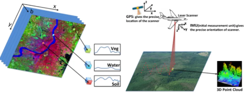
Hyperspectral imaging is categorized as passive sensing which gathers radiation that is emitted or reflected by the objects. Active sensing, on the other hand, emits energy to scan target objects then detects and measures the reflected or backscattered radiation from them. Synthetic aperture radar (SAR), Radar, and LiDAR are examples of active remote sensing. SAR imaging operates at the microwave range in the electromagnetic spectrum and can acquire data through clouds. A pixel in a SAR image may contain information such as radar backscattering intensity and phase, range measurement between the sensor and a reflecting object, etc. LiDAR instruments illuminate a target with a laser and analyze the reflected light. It measures the heights of objects and structures on the ground more precisely than using radar technologies. Also, it can make the three-dimensional positioning of objects in the scene well defined. LiDAR sensors are able to produce a 3D point cloud from which the Digital Terrain Models (DTM), Digital Surface Models (DSM) and 3D models of an object could be further calculated [3]. With the fast development of different remote sensors, the multi-modalities of remotely sensed data may promote the development of data fusion strategies for a better understanding of the area under investigation.

1.1.2 Remote Sensing Data Fusion

The multi-modalities of remotely sensed data provide more possibilities of information exploitation compared to a single data source. Different sensing devices capture different

(19)

CHAPTER 1. INTRODUCTION 18

physical characteristics of the same scene and combines to enhance the understanding of the target objects. They also provide the basis for discrimination, identification and characterization. Hyperspectral images have fine spectral resolution to determine and characterize different materials based on their spectral signatures. It may also provide the possibilities of extracting spatial information in the spatial domain. LiDAR sensors collect 3D point clouds that can be used to extract elevation and curvature information to further provide separabilities between different structures. Other than the emergence of multi-sensor data and multi-feature information, the multi-temporal data, revealed by the ambition of the remote sensing community to develop new generation of sensors, also has gained increased attention. The development of novel data fusion techniques to address new challenging applications is demanding.

Remote sensing data fusion aims to integrate multi-source information generated from different perspectives, acquired with different sensors or captured at different times in order to produce fused data that contain more enriched information than one individual data source. In this procedure, multiple data sources would result in an increase in data volume, dimensionality of the feature space, and interclass separability. For the clus-tering and classification tasks of remotely sensed data, especially the high dimensional HSI data, fusion strategies may also include the selection of a subset of features and the eliminating of redundant features. In machine learning and pattern recognition, the available data fusion techniques can be mainly classified into three categories, namely, low-level information/data fusion, intermediate-level feature fusion and high-level de-cision fusion. The low-level fusion combines multiple raw data sources to generate as new input data that takes the advantages of complementary or collaborative data sources. The intermediate-level feature fusion may include feature primitive identification, feature extraction/selection, and feature combination [4]. Compared to low-level pixels, feature primitives can include pixel intensity, edge, texture, shape, length or image segments, and etc. The identification and extraction of the feature primitives can generate higher level descriptions of the data, and can be fused as another information source to improve the data processing. Feature fusion also includes the selection and combination of features to remove redundant and irrelevant features for analysis. The integration of multiple data sources may easily result in high dimensional feature space and significant amounts of redundant information. Feature extraction/selection thereby refers to the step of

(20)

find-CHAPTER 1. INTRODUCTION 19

ing only those features that contain a significant amount of information. The high-level decision fusion takes advantage of multiple classifiers to provide better accuracy and efficiency in the final decision. There are varieties of classifiers such as Support Vector Machine (SVM), kernel-based SVM [5], k-nearest neighbor (KNN), Gaussian Maximum Likelihood (GMM), etc. Different classifiers may hold certain assumptions of the data, or involve parametric modeling that is data dependent. To avoid the disagreements between different classifiers, the utilization of multiple classifiers can provide better generaliza-tion. In certain cases, the quantity of data to be processed is too large to be handled simultaneously. A multi-classifier framework will be efficient in which the data will be processed as multiple subsets with different classifiers [6].

In practical applications, the above fusion categories does not encompass all fusion methods. Usually, the applied fusion procedure is a combination of different level of fusion techniques as described above. Based on the data sources and combinations, remote sensing data fusion may be broadly categorized as optical panchromatic (PAN) and HSI data fusion, spatial and spectral feature fusion, LiDAR point cloud and HSI fusion, Multi-temporal data fusion, etc. The purpose of fusing PAN and HSI image is to improve spatial resolution and retain the spectral fidelity of the original HSI data. This is also referred to as pan-sharpening in the literature. The spatial and spectral feature fusion aims to exploit the spatial information contained in the remote sensing spectral data, which is helpful for the discrimination of materials with different structure or shape in the scene. The extracted spatial features can also be identified as an additional data source, it then allows us to use the spatial and spectral information by means of multi-source fusion techniques. The fusion of LiDAR data and imagery such as HSI has been explored in recent years. A LiDAR point cloud is a good source for generating a highly accurate DSM model. The elevation and gradient information combined with detailed spectral knowledge can facilitate the data analysis in urban area, such as building footprint extraction, land cover mapping, forest boundary detection, etc. Multi-temporal images have gained attention in the remote sensing community recently. The fusion of multi-temporal images provides a new spatio-spectra-multi-temporal perspective of the remotely sensed data [7]. The multiple images captured at different time or using different sensors need to be properly aligned (i.e. the spatial co-registration and compensation for the changes). Other sources of remotely sensed data, for example, SAR, GIS data, range

(21)

CHAPTER 1. INTRODUCTION 20

sensors and digital photogrammetry [8], and etc., have been fused with HSI in many applications, such as environmental monitoring, object detection and 3D reconstructions. Overall, remote sensing data fusion is a demanding research field as the fast emergence of multi-modality data.

1.1.3 Data Modeling and Processing with Graphs

A graph is a powerful tool to model pairwise relationships between data points. It has wide applications in computer vision, machine learning, and image processing. For remotely sensed data, a graph can be used to model the pairwise relationship among neighboring pixels, 3D point clouds, regions or clusters, multiple features, and etc.

HSI data points can be individually represented by vectors in a high dimensional feature space. Intensive work has been performed for HSI classification and clustering during the last few decades. Parametric models, such as Gaussian maximum likelihood and linear discriminant analysis, have been investigated for the classification of spectral images [9]. These statistical parametric models based on the estimation of covariances and means, can successfully deal with multispectral images but are less reliable for hyper-spectral images due to their high dimensionality. Non-parametric and nonlinear models, such as Bayesian models, kernel methods and Support Vector Machines (SVM), Neural Networks and spectral clustering (as in spectral graph theory) have been investigated for hyperspectral data. In particular, spectral clustering, as a graph-based approach, has shown remarkable performance in terms of accuracy and simplicity. Graph models used in spectral clustering, with the useful mathematical tool such as the graph Laplacian, can transform HSI data into low-dimensional feature space where different clusters are more separable.

Spectral clustering is closely related to dimensionality reduction with graph repre-sentation [10]. The fusion of multiple data sources and features can easily result in high dimensionality which may gain much more computational complexity and suffer from the ”curse of dimensionality”. Graph representations of the data or features first build a neighborhood proximity graph in the high dimensional data space and embed this graph into a low-dimensional space and preserve most of the relationships among the original data. The purpose of a graph model used for dimensionality reduction is to provide a

(22)

CHAPTER 1. INTRODUCTION 21

non-parametric model with no statistical assumptions being made for the data.

The graph model can also be used to model the relationships between multiple data sources, such as multi-temporal images. Though correspondences are difficult to model due to changes in the environment, the intrinsic structures of classes contained in these sequential images are similar. Manifold alignment [11] constructs connections between disparate data sets by aligning their underlying individual manifolds and transferring information across the multiple data sets.

Additionally, data representation with a graph allows the possibility of performing combinatorial optimization to produce highly efficient solutions. For a binary case, the graph cut algorithm is the most well-known approach in computer vision that makes the energy-minimization problem directly translated to the minimum cut problem. Given a data set, data points can be efficiently labeled into two different groups by max-flow/ min-cut optimization. Beyond the binary case, the energy minimization problem can be considered a maximum a posteriori (MAP) estimation problem in a Markov random field (MRF) framework which is based on undirected graphical model. Overall, graph model is a powerful tool for describing and understanding the structure of the data in many applications as described above.

1.2

Objective and Contributions

Data fusion aims to integrate data from multiple sources to enrich the knowledge about the target, and to gain better interpretation and understanding of it. With the rapid development of multiple types of remote sensors and deep exploration of the multimodal remotely sensed data, data fusion becomes an effective and demanding technique for optimum utilization of the remotely sensed data with large volume.

Recently, graph-based data modeling and processing techniques have emerged as useful tools for image data analysis. Many real-world problems have been successfully modeled with graph-based approaches in the literature. The number of concepts and processing skills that can be solved with graph representation is very large. Therefore, graph theory has found many developments and applications in the image processing area due to the feasibility of modeling pairwise relationships for discrete data. Different

(23)

CHAPTER 1. INTRODUCTION 22

graph models have been proposed for image analysis, depending on the data structures and processing skills. Graphs not only provide an effective representation of the data, but also enable efficient graph-theoretical algorithms to process the data. Spectral methods, involving a graph Laplacian, directly take advantage of Eigen analysis using linear alge-bra. It has wide applications in clustering, dimensionality reduction and data alignment. Minimum cut/maximum network flow algorithms in graph theory can serve as a power-ful tool for exact or approximate energy minimization for binary or multi-class labeling problems. The graph may also be naturally used as an efficient data encoding approach for hierarchical data representation.

Overall, the main objective of this research is to use and explore the graph-based modeling and processing techniques for data fusion, particularly in remotely sensed multi-source data analysis. More specifically, the work proposed in this thesis is an attempt to exploit graph models under multi-source data and feature fusion framework:

• _{As an e}ff_{ective modeling method for the extraction of features related to the materials}

and objects in a given scene. Serves as a preliminary step for other applications, such as classification and detection.

• _{As a tool to represent and incorporate multi-source data into the framework for the}

image interpretation.

• _{Provide mathematical fundamentals for data embedding, feature selection}/_extraction

to reorganize input data and remove redundant information.

1.3

Outline of Thesis

This dissertation thesis summarizes the application of graph-based modeling and data fusion techniques on remotely sensed data clustering and classification. It is organized into six chapters that cover different topics related to the subject of interest in this research. 1. Chapter 2: An overview of data fusion strategies for remotely sensed data is presented in Chapter 2. With an increasing quantity of data captured by air-borne/satellite sensors, fusion in the four fields become popular: the multi-spectral

(24)

CHAPTER 1. INTRODUCTION 23

image pan-sharpening, spatial-spectral data fusion, LiDAR and image fusion, multi-temporal data analysis. The combination of multiple source of information can greatly enhance the performance of applications related to image interpretation and understanding. In this chapter, remote sensing data classification, particularly HSI data classification, are introduced and explained. The remote sensing data classification aims at grouping observations to represent land cover features. The techniques used for classification could be categorized as unsupervised or super-vised, pixel-level or object-level, etc.

2. Chapter 3: Graph theory has been widely used in data modeling and analysis for its strong mathematical foundation. In Chapter 3, the basic concepts and notations for spectral graph theory are explained. A topological algorithm that is purely based on a graph data structure is introduced for solving a HSI classification problem. Besides, the manifold learning techniques, which have been widely investigated for HSI data processing by represent ing the topology of the high-dimensional nonlinear data into a lower dimensional space, are discussed. An overview of manifold learning algorithms and their application to high-dimensional remotely sensed data are presented in this chapter.

3. Chapter 4: Spatial and spectral feature fusion in a manifold learning framework is described in Chapter 4. Remotely sensed data consists of a substantial amount of spatial and spectral information which brings a challenge to traditional image and signal processing. Methods for feature mining of HSI data are introduced to improve the use efficiency of the huge quantities of data. Algorithms based on improved affinity matrices that embedded with spatial and spectral information are proposed for efficient joint spatial-spectral HSI data clustering.

4. Chapter 5: High-order tensor is introduced for efficient multi-feature data repre-sentation. In HSI analysis, classification and segmentation usually represents each pixel as a vector in high-dimensional space and solves the mathematical problems use linear algebra, i.e., the algebra of matrices. Tensor-based image analysis has been explored in recent years. By adopting multilinear algebra, tensors can be effi -ciently used to combine multiple features, to represent super-pixels, and to reduce

(25)

CHAPTER 1. INTRODUCTION 24

the dimensionality of high dimensional data. In Chapter 5, algorithms for multi-feature fusion with high-order tensors are proposed and explained. Comparisons to traditional linear algebra based methods are provided.

5. Chapter 6: A summary of work in this dissertation is presented in the last Chapter. The insights, contributions and future work are also presented.

(26)

Chapter 2

Data Fusion and Classification in

Remote Sensing

The multi-modalities of remotely sensed data provide more possibilities of information exploitation compared to a single data source. The fusion of multi-source data can in principal produce more detailed information to characterize the objects. Furthermore, fusion techniques can also help with removing redundant and noisy information in the data. By applying data fusion methodologies, the performance of remotely sensed data classification may be significantly improved.

2.1

Multi-source Data Fusion in Remote Sensing

In the remote sensing research field, an increasing quantity of data captured by air-borne/satellite sensors has become available, including Very High Resolution (VHR) im-ages, multi-temporal imim-ages, multi-band imim-ages, multi-polarization imim-ages, SAR imim-ages, LiDAR point clouds, and others. The large amount of multi-source data makes remote sensing data fusion more demanding and challenging. Data fusion has gained its pop-ularity and usefulness in computer vision, machine intelligence, medical imaging and many other data processing areas. The objective of data fusion in remote sensing is to take advantage of multiple data sources to produce collaborative and complementary information for the interested scene than a single data source can provide. However,

(27)

CHAPTER 2. DATA FUSION AND CLASSIFICATION IN REMOTE SENSING 26

multi-source data fusion remains as a challenging task due to the existence of variations within different input data sets and the requirement for accurate data co-registration. Other than the data captured with different sensors, high-level features may be extracted from the original remote sensed data and combined into one or more feature maps that can be used as complementary data sources to the original data. For example, with recent remote sensors, the acquired multi-band images have very fine spatial resolution. The useful spatial feature information may be extracted as an independent data source that adds extra contextual information to the original spectral information. Therefore, the multi-sensor data and generated high-level feature data allow the possibility to exploit the remote sensing data by means of multi-source fusion strategies. According to the data sources, the fusion strategies for remotely sensed data are in the four fields: the multi-spectral image pan-sharpening, and spatial-spectral data fusion, LiDAR and image fusion, multi-temporal data analysis.

2.1.1 Remote sensing systems

Remote sensing aims at using aerial sensor technologies to detect and classify objects on Earth without being directly in contact with the target under investigation. Tremendous developments in the field of remote sensing have taken place in the past decades. Remote sensing is a remarkably broad subject including photographic imaging, nuclear magnetic resonance imaging, seismic tomography, multi-beam sonars, synthetic aperture radars, and etc. In this thesis proposal, we are particularly interested in the use of remote sens-ing data collected by airborne or spaceborne sensors for characterizsens-ing and classification of the Earth surface. Depending on the source of the energy involved in remote sens-ing data acquisition, two kinds of airborne imagsens-ing systems will be discussed, namely, passive and active systems. The outstanding representatives of the two systems are Hy-perspectral imaging and LiDAR. We will briefly review the sensor advances in the field of hyperspectral imaging and LiDAR , respectively.

2.1.1.1 Hyperspectral imaging systems

Hyperspectral imaging, also termed imaging spectroscopy, has been increasingly used in various applications, such as food safety, pharmaceutical process monitoring and quality

(28)

CHAPTER 2. DATA FUSION AND CLASSIFICATION IN REMOTE SENSING 27

control, biometric, forensic, and etc. The hypserspectral sensors acquire a spectral vector with hundreds of elements from every pixel in a given scene and result in a HSI cube. The spatial and spectral characteristics of HSI are similar to photographic images and videos, so that many tools developed for those data can be directly extended for HSI analysis.

The acquisition of hyperspectral images can be obtained by airborne or spaceborne platforms. Table 2.1 displays spatial and spectral parameters of eight existing or pro-posed hyperspectral sensors: two airborne (HYDICE and AVIRIS) and six spaceborne (HYPERION, EnMAP, PRISMA, CHRIS6, HyspIRI and IASI) [12]. From the table, it can be observed that the spatial resolutions are higher for sensors carried by lower altitude platforms. The number of bands for the first six sensors is approximately 200 with a spectral resolution of the order of 10 nm, which offer a huge potential to discriminate ma-terials. The last two sensors: CHRIS covers the visible bands and IASI covers the VNIR and the LWIR bands. Thereby, they offer the ability to estimate physical parameters such as temperature, moisture and etc.

Figure 2.1: Example of Hyperspectral imaging and LiDAR imaging.

2.1.1.2 LiDAR systems

LiDAR sensing uses light in the form of a pulsed laser to measure ranges (variable dis-tances) to the Earth. These light pulses, combined with other data collected by the airborne system, can generate precise, three-dimensional surface geometrical characteristics of the Earth. LiDAR systems for remote sensing are usually on airplanes and helicopters to be

(29)

CHAPTER 2. DATA FUSION AND CLASSIFICATION IN REMOTE SENSING 28 Parameter HY-DICE AVIRIS HYPER-ION

En-MAP PRISMA HyspIRI CHRIS IASI Altitude (km) 1.6 20 705 653 614 626 556 817 Spatial res-olution (m) 0.75 20 30 30 5-30 60 36 V:1-2 km; H:25km Spectral resolution (nm) 7-14 10 10 6.5-10 10 4-12 1.3-12 0.5cm−1 Coverage (µm) 0.4-2.5 0.4-2.5 0.4-2.5 0.4-2.5 0.4-2.5 0.38-2.5 and 7.5-12 0.4-1.0 3.62- 15.5(645-2760 cm−1) Number of bands 210 224 220 228 238 217 63 8461 Data cube size 200× 320× 210 512× 614× 224 660× 256×₂₂₀ 1000× 1000× 228 400× 880×₂₃₈ 620× 512×₂₁₀ 748× 748× 63 765× 120× 8461

Table 2.1: Parameters of eight Hyperspectral instruments.

used for acquiring data over broad areas. The common major components in a LiDAR system are Laser, scanner and optics, photodetector and receiver electronics, and a spe-cialized GPS receiver. Two types of LiDAR are topographic and bathymetric. Airborne topographic LiDAR generally uses a 1064 nm near-infrared laser to map the land, while bathymetric LiDAR generally use 532 nm green light that penetrates water with much less attenuation, and measures seafloor and riverbed elevations.

In urban areas and forest study, the popular LiDAR sensors are those from the Optech ALTM-series, Leica ALS-series, RIEGL LMSseries, and the TopoSys Falcon series [13]. The basic measurement made by a LiDAR instrument is the distance between the sensor and a target surface by determining the elapsed time between the emission and arrival of the reflectedlaser pulse. Key differences among LiDAR sensors are related to the laser’s wavelength, power, pulse duration and repetition rate, beam size and divergence angle, the specifics of the scanning mechanism, and the information recorded for each reflected pulse [14]. LiDAR data has been used in measurement of the three-dimensional structure

(30)

CHAPTER 2. DATA FUSION AND CLASSIFICATION IN REMOTE SENSING 29

of vegetation canopies, prediction of forest stand structure attributes, building footprint extraction, forest delineation, road detection, and etc.

2.1.2 Spatial-spectral data fusion

Besides detailed spectral information, HSI also contains much contextual information. For a given pixel, we can extract the shape, size and texture information of the structure to which it belongs. This information will complement the spectral signatures to help discriminate and identify different objects in a scene. Consequently, a joint spatial-spectral data fusion strategy is needed to generate more accurate results in HSI image segmentation and classification.

Several methods have been explored to add spatial information to improve the re-mote sensed data classification and clustering. One of the earliest proposed classifier that used both spectral and contextual information is known as the ECHO classifier [15]. It is a multi-stage classifier based on texture segmentation and statistical classification. It is hypothesized to work well where classes of interest are widely mixed with high vari-ance. Later, Markov Random Field (MRF) was investigated in textural discrimination for remote sensing image segmentation [16, 17, 18]. An extensive literature is available on MRF modeling successfully applied in remote sensing image classification. In the MRF framework, the maximum a posteriori (MAP) decision rule is typically formulated as an iterative optimization step of the energy function, which is extremely time consum-ing with high resolution data. Furthermore, classical models used in MRF framework (e.g., Ising, Potts model) suffer from the high spatial resolution: neighboring pixels are highly correlated, while the standard neighbor system definition does not contain enough samples to be effective [19].

In addition, Rellier et al. [20] performed texture analysis using parameters employed by MRF to allow the characterization of different hyperspectral textures. Other than the MRF based texture analysis for hyperspectral image clustering and classification, various methods have been reported to extract the texture feature from the image region. Pixel shape index (PSI) [21] and the grey level co-occurence matrix (GLCM) [22] methods both start from a pixel in a given position then exploit the structural and shape information in outward directions in its neighborhood to complement the spectral feature space. Another

(31)

CHAPTER 2. DATA FUSION AND CLASSIFICATION IN REMOTE SENSING 30

model for extracting texture information, based on multiple 3D Gabor filters, captures the specific orientation, scale, and wavelength properties of hyperspectral data [23]. Similarly, wavelet analysis was also successfully utilized for hyperspectral image texture feature extraction [20, 24]. One of the most important aspects of texture description has been identified as the scale factor, and wavelet decomposition is able to generate a number of homogeneous features that represent the response of a bank of filters at different scales.

The other approach comprises multi-scale techniques as well as an adaptive neigh-borhood of a pixel according to the structures to which it belongs and was proposed by Benediktsson, et al [25]. They have exploited the morphological filters as an alterna-tive way of performing joint spatial-spectral classification. Rather than defining a crisp neighbor set for each pixel, morphological filters enable the definition of an adaptive neighborhood of a pixel according to the size and shape of the structures to which it belongs. This adaptive neighborhood approach has shown its good performance for multispectral and hyperspectral data [26]. Recently, M. Dalla Mura et al. [27, 28] inves-tigated the connected morphological operators for the analysis of very high resolution images, as well for HSI as an extension of the morphological profile based on a series of attribute filters. The attribute filters permit new possibilities for extracting morphological information in a way as it filters the spatial structures according to geometry (area, length, shape factors), texture (range, entropy), etc. Therefore, the input image can be processed according to different attributes, which can be defined with great flexibility.

2.1.3 LiDAR and image data fusion

The availability of LiDAR data has provided a new possibility for data classification and segmentation. Unlike optical and microwave sensors, LiDAR sensors directly measure both the vertical elevation and horizontal distribution of objects in a scene. The time interval between a laser pulse being emitted and retrieved can be measured by two approaches, namely, pulsed ranging (scanning LiDAR) where the travel time of a laser pulse from a sensor to a target is recorded, and continuous wave ranging (profiling LiDAR) where the phase change in a transmitted sinusoidal signal is converted into travel time [29].

(32)

CHAPTER 2. DATA FUSION AND CLASSIFICATION IN REMOTE SENSING 31

the remote sensing community. Images can provide detailed spectra for the discrimination of different materials in a study area, while LiDAR data can be exploited for characterizing topographical information of the scene. A single data source is difficult to provide reliable understanding of the scene. An image alone may not be able to differentiate objects of the same material, and LiDAR data alone provides little information for objects of similar geometrical structure with different material attributes. The fusion of LiDAR and imagery has been explored for a variety of applications such as DEM model generation, urban modeling, land cover classification, and etc.

The traditional approaches to generate DEM model are mostly based on stereo image matching. LiDAR sensors provide the capability of high-density 3D point data acquisi-tion. The use of LiDAR data for DEM model generation becomes an effective alternative approach to traditional stereo matching based methods [29]. Another application of fusing LiDAR data and aerial images is 3D object detection and extraction, particularly for building footprints and roads in urban modeling. Rottensteiner et al. [30] suggested LiDAR and aerial imagery fused to improve the degree of automation and robustness for building extraction. Much research in building extraction and reconstruction using LiDAR and image fusion skills has shown to improve height accuracy and building out-lines [31, 32, 33]. LiDAR data combined with imagery also works well for road extraction which is easily obscured by higher objects and difficult to accurately extract [34, 35].

The fusion of LiDAR and spectral image for land cover mapping has gained attention recently. The joint use of HSI and LiDAR data for the classification of forest areas, urban areas, and identification of trees from urban areas have been studied [3, 36, 37]. The previous works showed the incorporation of LiDAR source additionally improve the classification accuracy with extracted higher level features including curvatures and height information. Debes et al. [38] proposed a two-stream classification framework which takes advantage of both unsupervised segmentation and supervised classification using Random Forest classifier and combined with an object-level refinement to further enhance the accuracy for urban area data fusion. Liao et al. [38] adopted a graph-based framework to combine and embed spatial, spectral and LiDAR data in a lower dimensional manifold, followed by the classification with RBF-kernel based SVM.

(33)

CHAPTER 2. DATA FUSION AND CLASSIFICATION IN REMOTE SENSING 32

2.1.4 Multi-temporal data analysis

In recent decade, there has been a significant increase in the interest in multi-temporal data analysis in the remote sensing community. The successful launching of the Sentinel-1 in 2014 and the launching of the coming satellites of the Copernicus program, result in great demand for development of multi-temporal data analysis.

Multi-temporal data has been used for change detection for decades. Change detection can be broadly characterized into two groups [39]: bi-temporal change detection and temporal trajectory analysis. The former category focuses on comparisons between two dates, while the latter one emphasizes more on discovering the trend of change by creating “profiles” of multi-temporal data.

Given the variations within time period, difficulties are encountered in accurate mod-eling and mapping of urban and forest areas. Hemissi et al. [40] proposed an advanced form of the temporal spectral signature defining the reflectance for each data point as a congregation of the spatio-spectra-temporal dimensions. Fusion of multi-temporal im-ages facilitate the modeling of variations in spectral response due to time changes, and has proven to be effective in many applications [41, 42].

The multi-temporal Classification of remotely sensed image data takes advantage of efficient combination of different sources of information, namely, temporal, contextual, and multi-sensor to improve the results. Given an image labeled data, the problem of classifying another image of the same area obtained at a different time could be solved by passing the knowledge between the multi-temporal images. Many multi-temporal supervised methods have been developed, such as evidence reasoning [43], neural net-works [44], and Bayes rule [45]. Also, since the intrinsic structures in these sequential images are similar, the spectral variations across a series of images can be efficiently re-duced by grouping spectral neighbors within each image and mapping these clusters into a common space under a manifold alignment framework [46].

2.1.5 Multi-spectral image pan-sharpening

Multispectral (MS) imaging affords detailed spectral resolutions from visible to LWIR wavelength region with enhanced discriminating power for material identification and classification. One shortcoming of MS is the spatial resolution is usually coarser than

(34)

VHR panchromatic image. To overcome the limitations due to lower spatial resolution, fusion of MS data and high resolution panchromatic image can be adopted for enhanced performance. Due to the fact that the fusion of a MS with a high resolution panchromatic image is to improve the spatial resolution of it, we usually refer the process as pan-sharpening.

A panchromatic imaging detector has a single sensor which is sensitive to radiation within a wide spectral range, typically the visible part of the spectrum. Pan-sharpening is a pixel-level data fusion technique which fuses a PAN image and an HSI image to obtain one image with both high spatial and spectral resolutions. The pan-sharpening algorithms can be broadly categorized into three classes [47]: the component substitution (CS) fusion techniques, modulation-based fusion techniques and multi-resolution analysis (MRA)-based fusion techniques.

The CS method first up-samples the low-resolution MS image to have the same spa-tial size of the co-registered PAN image. Afterwards, with desired forward transform applied on the MS image, one component in the transformed image will be substituted by the PAN image which has higher spatial resolution. One classical CS pan-sharpening algorithm is the intensity-hue-saturation (IHS) transform [48] algorithm, in which the for-ward transformation of MS image is to obtain its components in the IHS space. The final pan-sharpened image is then generated by replacing the intensity component with the PAN image followed by an inverse IHS transform. Spectral distortion may occur in the fusion process, and various attempts have been made to minimize the spectral distortion in IHS pansharpening [49]. Other famous pan-sharpening algorithms, such as principal component analysis (PCA) transform fusion methods [50], Gram-Schmidt (GS) spectral sharpening algorithm [51], etc., still suffer from spectral preserving issues.

The modulation-based fusion methods are based on the idea that the spatial informa-tion is modulated into the MS images by the multiplicainforma-tion of the MS image with the ratio of the PAN image to the synthetic image. One typical modulation-based pan-sharpening algorithm includes Brovey transform (BT) algorithm [52], in which the synthetic image is the average of the blue, green and red bands.

The MRA-based fusion methods utilize multi-scale decomposition techniques such as Laplacian pyramids [53], multi-scale wavelets [54] and etc., to decompose MS and PAN images in different levels and apply a fusion rule onto the transform coefficients.

(35)

CHAPTER 2. DATA FUSION AND CLASSIFICATION IN REMOTE SENSING 34

2.2

Classification of remotely sensed image data

Remote sensing data classification, particularly HSI data classification, has been a very active area of research in recent years. Given a set of observations (i.e., pixel vectors, LiDAR point clouds), the objective of classification is to find the hidden structure in unlabeled data with or withouta prioriknowledge. In remote sensing data classification, the objective is to group observations to represent land cover features. Examples of land cover could be forested, urban, agricultural and other types of features. The techniques used for classification could be categorized as unsupervised or supervised, pixel-level or object-level, etc. Unsupervised classification, which may also be called segmentation or clustering, is the partitioning of data into related regions. It is an important first step for other applications in data analysis and compression. Also, due to the scarcity of labeled data and large dimensionality of the input data, unsupervised segmentation of remotely sensed data is more demanding. Supervised classification takes full advantage of available training data to learn and discover the underlying structure for the unlabeled data, which usually produces better accuracy compared to unsupervised segmentation algorithms. For HSI data, traditional supervised and unsupervised classification are based on the observation of spectral feature vectors for each pixel. In other words, those traditional techniques are all pixel-based, which do not utilize the local spatial information that can only be extracted at object-level, i.e., texture, shape, size, and etc.

2.2.1 Unsupervised classification

Unsupervised classification, or segmentation, aims to extract regions by dividing pixels into disjoint sets of segments. The segments should have the property that regions are “homogeneous” within the segments and “heterogenous” between the clusters. As an initial processing step, segmentation usually facilitates easier analysis of higher level applciations, such as anomalous object detection, image retrieval, compression, and etc.

Two broad approaches to remote sensing data segmentation are threshold-based and pixel clustering. In grayscale and binary image segmentation, threshold-based approach is useful in discriminating foreground from the background. By selecting an appropriate threshold value, the gray level image can be converted to binary image. Similarly, remote

(36)

sensing data, such as HSI, may be segmented into non-overlapping regions via threshold-based method. In [55], a manual multithresholding (MT) approach was proposed to segment HSI into different regions. They first extract spectral index (SI) image from HSI as a way to capture one or more spectral characteristics. Afterwards, the SI image is segmented into clusters by simply slicing the SI value into intervals of equal width. If a spectrum’s SI value lies in the first interval, it is classified to region 1; if it lies in the second interval, it is classified to region 2; and so on. The segmentation problem becomes the selection of proper value for the thresholds. The threshold selection techniques can further be categorized into local/global, simple/adaptive methods. Global threshold selection finds one simple threshold value for the entire image data set, whereas local threshold selection usually adaptively calculates the threshold for different pixels [56]. However, threshold-based techniques, although computationally less expensive, did not get much attention. Threshold-based techniques inherently work well with grayscale image while the remote sensed imagery of interest here usually contains multiple spectral bands. Other than that, the multi-dimensional spectral vector associated with each pixel naturally makes each of the pixel an individual feature instance and suitable for pixel-based clustering.

Pixel-based clustering groups pixels into homogeneous regions by clustering their feature vectors. The multi-band nature makes pixel-based clustering the natural choice for segmentation. The simplest and most commonly used methods for remote sensing data arek-means and ISODATA algorithms. Both of them are based on statistical modeling of the data to iteratively find the optimum partition of the data. In general, these two methods start by randomly picking several data points as the cluster center candidates and assigning each pixel to the closest candidate. Then statistical parameters are re-calculated and new cluster centers are updated based the new clusters. This process iterates until variations are below a certain threshold. Other statistical based algorithms applied to HSI data include the Gaussian mixture models [57].

Other than statistical based clustering algorithms, spectral clustering (SC) has been recently investigated for HSI pixel clustering. Compared to traditional clustering algo-rithms, SC has some obvious advantages. It is highly related to manifold learning which studies the underlying structure by modeling the pairwise relationship between pixels. Therefore, it facilitates the recognition of clusters of unusual shapes. On one hand, SC

(37)

CHAPTER 2. DATA FUSION AND CLASSIFICATION IN REMOTE SENSING 36

serves as a graph-based embedding which implies a clustering condition. On the other hand, SC seeks to find a clustering condition that can capture flat, elongated and even curved nonlinear data clusters.

2.2.2 Supervised classification

Supervised classification approaches first learn from an available training set to under-stand the statistical or geometrical characteristics of the clusters that exist in the data set. Once trained, the classifier is used to assign labels to unlabeled data points according to the learned knowledge of the data set. Traditional supervised classification methods for remote sensing data are pixel based on the spectrum of each pixel itself. Spatial information can be fused to the classification process by separately extracting spatial con-tents from neighboring pixels to be combined with spectral knowledge. The object-based classification methods usually work in the same way as a pixel-based classification, with the difference that we utilize image segmentation results as the input to the classifier. Therefore, object-based classification methods inherently contain higher-level informa-tion, such as statistical parameters, texture, shape, and etc., that can only be characterized at the object level instead of from individual pixels.

2.2.2.1 Pixel-level classification

For remote sensed data, especially HSI, the multi-dimensional spectra naturally makes each of the pixels an individual feature instance. In other words, pixel-level classification of an image is to categorize single pixels into land cover classes with only the spectral information for each pixel utilized as its feature vector. With a lack of neighboring information to each pixel, there usually exists a ”pepper and salt” phenomenon in HSI classification map.

One of the earliest and widely used supervised classification algorithm for remote sensing data is the Gaussian Maximum Likelihood (GML) classifier, which is based on Bayesian probability theory and has become a widely accepted statistical model for re-motely sensed data. It first learns and establishes a multi-dimensional histogram for each class from the training data, and assigns unlabeled data to classes based on a posteri-ori probability. The main problem involved in the probabilistic model is that the limited

(38)

CHAPTER 2. DATA FUSION AND CLASSIFICATION IN REMOTE SENSING 37

availability of training data may result in overfitting. The other problem is the underlying data distributions of the classes do not necessarily satisfiy a normal distribution.

Artificial neural network (ANN) classifier is one of the most widely used nonpara-metric classification algorithm in pattern recognition field. It usually consists of one input layer, at least one hidden layer and one output layer. The ANN may be able to handle non-normal, complex feature spaces and multivariate data types. In the literature, it also has been found that the difference between the performances of other classifiers and ANN increase in favor of ANN with the increasing number of channels. One important prop-erty of ANN classifier is, with a sophisticated paradigm, it can handle data with a small training set. However, with high-dimensional input data, the complexity dramatically increases in ANN classifier. Therefore, dimensionality reduction is frequently applied to high dimensional data to achieve tolerable training time.

Support vector machines (SVM) have been investigated intensively as an alternative approach to the usual statistical and neural classifiers for high-dimensional images. The SVM classifier is based on the concept of a decision plane which identifies the boundary lines that separate a set of objects with different class labels. In order to handle nonlinear boundaries, ”kernel tricks” are widely adopted for SVM classifier to project the original data into a higher dimensional implicit feature space where classes are linearly separable. SVM appears to be advantageous compared to other supervised classifiers in the presence of heterogeneous classes with only small training set, and it is less sensitive to the curse of dimensionality. The other advantage of the SVM classifier is that it requires little effort for architecture design since it involves few control parameters. However, SVM was originally proposed to solve two-class problem. To effectively solve multi-class classification problem with SVM classifiers is still an ongoing research issue.

The Random forest classifier, as one of the ensemble methods, combines the predic-tions of several decision tree classifiers in order to improve generalizability over a single estimator. A decision tree classifier is advantageous to pixel-level remote sensed data classification because of its flexibility, intuitive simplicity and computational efficiency. It recursively partitions a data set into smaller subsets according to different criteria at each node in a tree structure. The classification procedure is strictly non-parametric and does not make assumptions of the data distribution. In random forest classifier, each decision tree in the ensemble is built from a sample of data points drawn with replacement from

(39)

CHAPTER 2. DATA FUSION AND CLASSIFICATION IN REMOTE SENSING 38

the training set. In the final step, every pixel is classified based upon a majority vote from all the tree predictors used in the forest to obtain its final label.

2.2.2.2 Object-level classification

In object-leveled classification, the input processing units are no longer single pixels but image objects. In order to apply object-level classification, first the remote sensed data points needs to be grouped into meaningful clusters based on their individual features. Secondly, the clusters need to be effectively represented and used as the input instances to the classifiers with different region-level classification rules, such as spectral, spatial, contextual and textual information. Thereby, the obvious advantages of object-level classification to the conventional pixel-object-level classification is the incorporation of additional information, namely, texture, shape, size, and etc., which can only be extracted at object-level. The other advantage of object-level classification is the spectral properties of individual pixel are averaged for the object or structure it belongs to. Because spectral mixing increases in a remotely sensed image that has coarse spatial resolution, this may cause confusion in the classification. By extracting and averaging the spectral information at object-level, the within-object variability can be reduced.

In general, object-level classification includes an unsupervised multi-resolution seg-mentation and a knowledge-based classification. The classification can usually adopt the general classifiers as mentioned above. The multi-resolution segmentation starts from treating each pixel as a separate object and gradually combining them into regions. One commonly used technique for multi-resolution segmentation is bottom-up merging which iteratively groups adjacent and similar pixels into meaningful objects. Subsequently, ad-jacent and similar image objects are merged to form bigger ones based on object-level similarity measure until stopping criterion is met.

Recently, geographic object-based image analysis (GEOBIA) has become a new dis-cipline for the analysis of remote sensing data. This is a sub-disdis-cipline of Geographic Information Science (GIScience) devoted to developing automated methods to partition remote sensing imagery into meaningful image-objects, and assessing their character-istics through spatial, spectral and temporal scales, so as to generate new geographic information in GIS-ready format [58]. In this new discipline, many theories, methods and

(40)

CHAPTER 2. DATA FUSION AND CLASSIFICATION IN REMOTE SENSING 39

tools have been developed to replicate human interpretation of remote sensed images in automated/semi-automated ways. Overall, object-level analysis of remote sensed images offers new possibilities for situations where spectral properties are not unique, but where shape or neighborhood relations are distinct. Also, object-level processing is closely re-lated to human cognitive perception of the scene compared to pixel-wise understanding of the image.

2.3

Summary

This Chapter introduced the data fusion strategies for remotely sensed data and ad-dressed the classification problem in remote sensing area. The development in remote sensing tools and technologies provide more possibilities in data fusion. The high spatial resolution in hyperspectral imaging enables spatial feature mining, so that features from spatial domain be exploited simultaneously with the detailed spectral information. Li-DAR