The Effect of Several Tradeoffs in the
Implementation of Large Displays on
the Performance of the Users of the
Displays
by
Shivam Dembla
A thesis
presented to the University of Waterloo in fulfillment of the
thesis requirement for the degree of Master of Applied Science
in
Systems Design Engineering
Waterloo, Ontario, Canada, 2015 c
Author’s Declaration
I hereby declare that I am the sole author of this thesis. This is a true copy of the thesis, including any required final revisions, as accepted by my examiners.
Abstract
A large display can be constructed in two different ways:
1. a rectangular grid, or tiling, of many small screens with seams, or bezels, at the boundaries between the screens and
2. one large screen with no bezel inside the screen.
The first way costs significantly less than the second way. However, the first way creates a discontinuity in the image because of the bezels, and this discontinuity may impact a user’s performance.
There are two different ways to implement the first, tiling way of constructing a large display:
1. tiled, multiple projections onto one large screen and 2. tiling of actual LC displays.
With the first way, bezels are avoidable, but there is the necessity of continuous, precise coordination of multiple projectors. With the second way, once the displays are mounted, no coordination is necessary, but bezels are unavoidable.
While it might seem preferrable to avoid bezels and incur higher construction or coor-dination costs, the reality is that if no user’s performance is negatively affected by bezels, then there is no reason not to use the cheaper methods of constructing large displays.
Therefore, the aim of this study is to determine how bezels affect a user’s task perfor-mance. We conducted two controlled experiments in order to determine
• how varying the width of bezels affects a user’s performance; • how varying the number of bezels affects a user’s performance; and
• how the choice between tiled, multiple projections and tiling of actual LC displays affects a user’s performance.
In each experiment, the participants solved a puzzle within a given time. The findings from this study are that user performance is not affected by variation in the width of bezels and by variation in the number of bezels. However, the tiling of actual LC displays is better for user performance than tiled, multiple projections.
Therefore, it is more acceptable to use a rectangular grid of actual LC displays to implement a large display.
Acknowledgements
Firstly, I would like to thank my advisor, Dr. Daniel M Berry and my co-supervisor Dr. John Zelek for providing continuous support and guidance throughout my Master’s program for 2 years. I could not have imagined having better advisors and mentors for my master thesis. I am also grateful to them for giving me the freedom to choose the research problem and also offering me necessary guidance in my approach to analyze and solve it.
I would like to express my gratitude to Dr. Chrysanne Di Marco and Dr. Michael Terry for taking the time to read my thesis. I would like to mention Dr. Stacey Scott and Dr. Mark Hancock for their support during the study. Special thanks to my friends with whom I started my journey at University of Waterloo (in alphabetical order), Karan, Rakesh, Rupinder, Sandeep, Shrinu, for all the insightful discussions in work and on personal front. I am also indebted to my cousins: Anchal and Shruti and to my friends: Sri Harsha, Vijith for making my stay at waterloo a memorable one.
Also, many thanks to Nicole Keshav and my friend Jyoti Sahu who helped in editing my thesis and always there to support me.
Finally, I would like to thank my parents and my lovely elder sister, my nephews for supporting me all these years while pursuing my dreams.
Dedication
Table of Contents
List of Tables viii
List of Figures x
1 Introduction 1
2 Related Work 8
2.1 Construction . . . 8
2.2 Overlay and offset . . . 9
2.3 Navigation . . . 9
2.4 Aesthetics of the display . . . 11
2.5 Effects of bezel . . . 11 2.6 Conclusion . . . 13 3 Experimental setup 15 3.1 Bezel experiment . . . 15 3.1.1 Projector display . . . 15 3.1.2 LC display . . . 16 3.2 Bezel width . . . 18 3.3 Experimental task. . . 19 3.4 Participants . . . 19
4 Results 24
4.1 Projector display analysis . . . 24
4.2 LC display analysis . . . 31
4.3 LC display versus projector display . . . 43
5 Discussion 48
6 Future Work 51
List of Tables
3.1 Design of Experiments - Projector Display . . . 22
3.2 Design of Experiments - LC Display . . . 23
4.1 Participants’ Task Completion Percentages - Projector Display . . . 25
4.2 ANOVA Mean and Variance for complete data set . . . 26
4.3 ANOVA Analysis for complete data set . . . 26
4.4 Mean and Variance of data set keeping number of screens = 4 and varying width of Bezel . . . 27
4.5 ANOVA Analysis of 4.4 . . . 27
4.6 Mean and Variance of data set keeping number of screens = 9 and varying width of Bezel . . . 27
4.7 ANOVA Analysis of 4.6 . . . 29
4.8 Mean and Variance of data set keeping number of screens = 16 and varying width of Bezel . . . 29
4.9 ANOVA Analysis of 4.8 . . . 31
4.10 Mean and Variance of data set keeping width of the Bezel = 0.5cms and varying number of screens . . . 31
4.11 ANOVA Analysis of 4.10 . . . 33
4.12 Mean and Variance of data set keeping width of the Bezel = 1.0cm and varying number of screens . . . 33
4.13 ANOVA Analysis of 4.12 . . . 34
4.14 Mean and Variance of data set keeping width of the Bezel 2.0cms and varying number of screens . . . 34
4.15 ANOVA Analysis of 4.14 . . . 34
4.16 Participants’ Task Completion Percentages - LC Display . . . 35
4.17 ANOVA Mean and Variation for complete data sets . . . 36
4.18 ANOVA Analysis for complete data set . . . 36
4.19 Mean and Variance of data set keeping number of screens = 4 and varying width of Bezel . . . 38
4.20 ANOVA Analysis of 4.19 . . . 38
4.21 Mean and Variance of data set keeping number of screens = 9 and varying width of Bezel . . . 40
4.22 ANOVA Analysis of 4.21 . . . 40
4.23 Mean and Variance of data set keeping number of screens = 16 and varying width of Bezel . . . 42
4.24 ANOVA Analysis of 4.23 . . . 42
4.25 Mean and Variance of data set keeping width of the Bezel = 0.5 cms and varying number of screens . . . 43
4.26 ANOVA Analysis of 4.25 . . . 43
4.27 Mean and Variance of data set keeping width of the Bezel = 1.0 cms and varying number of screens . . . 45
4.28 ANOVA Analysis of 4.27 . . . 45
4.29 Mean and Variance of data set keeping width of the Bezel = 2.0 cms and varying number of screens . . . 46
4.30 ANOVA Analysis of 4.29 . . . 46
4.31 Mean and Variance of data set keeping width of the Bezel = 4.0 cms and varying number of screens . . . 47
List of Figures
1.1 High and low resolution image [2] . . . 3
1.2 The difference in the resolution of one single contagious display . . . 3
1.3 Overlay approach . . . 5
1.4 Offset approach . . . 5
1.5 Image before OneSpace adjustment . . . 6
1.6 Image after OneSpace adjustment . . . 6
2.1 Mouse tail . . . 14
3.1 Tiled monitor configuration used in experiment [2x2] . . . 17
3.2 Tiled monitor configuration used in experiment [3x3] . . . 17
3.3 Tiled monitor configuration used in experiment [4x4] . . . 20
3.4 Dimension of large projector display. . . 20
4.1 Distribution of data set 4.4 keeping the number of screens = 4 and varying the width of bezels . . . 28
4.2 Distribution of data set 4.6 keeping the number of screens = 9 and varying the width of bezels . . . 28
4.3 Distribution of data set 4.8 keeping the number of screens = 16 and varying the width of bezels . . . 30
4.4 Distribution of data set 4.10 keeping the width of the bezel = 0.5cms and varying the number of screens . . . 30
4.5 Distribution of data set 4.12 keeping the width of the bezel = 1.0cm and varying the number of screens . . . 32
4.6 Distribution of data set 4.14 keeping the width of the bezel = 2.0cms and varying the number of screens . . . 32
4.7 Distribution of data set 4.19 keeping the number of screens = 4 and varying the width of bezels . . . 37
4.8 Distribution of data set 4.21 keeping the number of screens = 9 and varying the width of bezels . . . 37
4.9 Distribution of data set 4.23 keeping the number of screens = 16 and varying the width of bezels . . . 39
4.10 Distribution of data set 4.25 keeping the width of the Bezel = 0.5cms and varying the number of screens . . . 39
4.11 Distribution of data set 4.27 keeping the width of the Bezel = 1.0cm and varying the number of screens . . . 41
4.12 Distribution of data set 4.29 keeping the width of the Bezel = 2.0cms and varying the number of screens . . . 41
4.13 Distribution of data set 4.31 keeping the width of the Bezel = 4.0cms and varying the number of screens . . . 44
4.14 Task completion percentage in LCD and projector display . . . 44
Chapter 1
Introduction
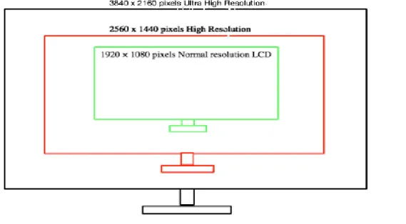
Large and high resolution displays have become ubiquitous. They are becoming common in various fields such as geo-spatial, military, and automotive design [18], among other fields. They are useful in navigation [13], advertising/public display [25], 3D viewing without glasses [46], displaying large data sets in scientific visualization [39], conferences, meetings [28], and many other applications in which data sets are required to be visualized minutely and in large contexts. Displays can be low resolution1, high resolution2, and ultra high resolution3. The range of pixels in display varies from a few thousand pixels to billions of pixels. Examples of displays include mobile phones, tablets, laptops, desktop displays, tiled monitor displays, and billboard displays. This thesis uses the following terminology for describing displays:
• Size of a screen is measured diagonally in inches or centimetres.
• Resolution is the number of vertical pixels multiplied with the number of horizontal pixels.
The advantage of greater resolution is having more information displayed at once. However, arbitrarily increasing the resolution of a display and keeping the size of the display fixed is not reasonable because at some point, the visual acuity of the user cannot make use of the increased resolution. We limit the resolution of the display so that a user’s visual acuity can utilize the information on the display. The world’s current highest resolution wall has
1at current standards, 2-4 million pixels approximately 2at current standards, 5-8 million pixels approximately 3at current standards, more than 8 million pixels
been developed by the University of California at San Diego. It is the Highly Interactive Parallelized Display Space (HIPerSpace) [6] featuring 286.7 million pixels, which is 30 million pixels more than the NASA hyper-wall-2 (256 million pixel system) constructed by NASA Ames Research Centre [48].
Large displays are gaining importance because of their affordability and their ability to display granularity. Having a large display does not mean covering only one wall and displaying information. There are displays covering five walls [58] and those covering six walls [44]. There are also screens which can support the weight of a user.
There are two ways to construct a large displays. 1. A single continuous screen.
2. A collection of smaller displays laid out in a rectangular grid with all the needed pixels. The boundaries of the smaller screens create a discontinuity in the display. One such boundary is called a bezel, and it has a non-zero width.
An example of each is
1. A single 9600X5400 display with 51.8 million pixels, and
2. A 5x5 grid of 25 1920X1080 displays with the same 51.8 million pixels.
Observe that they have the same resolution and that the second has four horizontal bezels and four vertical bezels. The first kind of display is available in limited pixels up to a few million and costs around $25,000 to $500,000. LG’s 84 inch diagonally and 8.3 million pixel display costs around $25,000. Tiling five monitors, each of size 21 inch diagonally and of resolution 1680 by 1050 per monitor, for a total of 8.8 million pixels costs around $2,500. The cost of a tiled-monitor display is one tenth of the cost of single display with almost the same resolution.
In the second way to implement a large display, the discontinuity in the image at the bezels might bother the users. However, if the users are in fact not affected by the presence of bezels, then the choice is clear. Go for the cheaper method of making a grid of smaller displays and make the seams as small as possible.
Within the second choice of a grid of smaller displays, there are yet two more tradeoffs: 1. The grid is made of liquid crystal (LC) displays with physical bezels, and
Figure 1.1: High and low resolution image [2]
2. The grid is made of projectors projecting on to a large enough undivided screen with virtual only bezels in it.
The tradeoffs between these two choices are:
1. With a projector display, we can achieve a display with almost no bezels, but it comes with the cost of calibration of the positions and brightness of the individual projectors [39], many projectors, and a large projection screen. The setup is bulky and the cost of setting up a projector display is higher than tiling LC displays [39]. 2. A tiled LC display has physical bezels in it, which are unpleasing [15], but it is easier
to build because there are fewer calibration issues than for a projector display. These displays can be vertical as mounted on wall displays or horizontal as on table tops. There are two ways of implementing the discontinuity of the image caused by the bezels. 1. Offset: In offset, the pixels to the left or the top of a bezel are adjacent in the image
to the pixels to the right or the bottom of the bezel. Thus, there is a gap between adjacent pixels in the image at each bezel.
2. Overlay: In overlay, there is no gap between adjacent pixels in the image, and a bezel hides a strip of the bezel’s width of the image.
In overlay, as shown in Figure 1.3, parts of the image are hidden behind the bezels, and that might create a problem in a user’s understanding the displayed image. Overlay is described by Almeida’sFrench Window is discussed in Chapter2. In our experiments, we use the overlay implementation of bezels because this implementation is the most common in commercial large displays.
In offset, Figure 1.4, the path of a mouse is deflected because of the gap in the image [43]. Offset not only deflects the mouse’s path, but it also distorts images and it may make documents confusing [15]. Robertson et al. tried to eliminate the warping effect and keep the trajectory of the mouse in line with the previous screen [43]. Similarly, an image that is distorted by bezels is corrected by a technique called OneSpace. In OneSpace, a user adjusts an image once for a given display to inform the system about the exact bezel placement. This technique hides the part of image located behind the bezel but lets the user to see a distortion-free image [43]. See Figure 1.6 and Figure 1.5. Offset does not
Figure 1.3: Overlay approach
Figure 1.5: Image before OneSpace adjustment
create much distortion when there is some video-related task. The human brain can make up the portion hidden behind the bezel.
How these tradeoffs affect users gives rise to the following research questions: • How worthwhile is it to invest in eliminating bezels?
• In a situation in which a large high-resolution display is needed by humans to perform a task with images, does the presence of bezels affect the users’ performance of the task?
• How does the width of the bezels affect the users’ performance? • How does the number of bezels affect the users’ performance?
• Which implementation of a grid of displays is better from the users’ viewpoint: LC display or projection?
The rest of this thesis uses “performance” to include all aspects of a user’s performance of his or her task, including throughput, task completion time, and error rate. A higher performance means a greater throughput, a shorter task completion time, and a lower error rate. There are yet other issues, but addressing them is declared beyond the scope of this research. These research questions give rise to the following hypotheses to be tested by experiments:
• H10: User task performance is not affected by increasing the width of bezel. • H11: User task performance is affected by increasing the width of bezel.
• H20: User task performance is not affected by increasing the number of bezels. • H21: User task performance is affected by increasing the number of bezels.
For anyHn, Hn0 is the null hypothesis, and Hn1 is its corresponding non-null hypoth-esis. We present the results of two user studies that investigate the effect of bezel width and number of bezel on users’ performance and compare LCD and projector display from users’ view point.
The following sections provide an overview of the related work, explain issues related to bezel display, and describe the experiments. The thesis concludes with the results, discussion, and future work.
Chapter 2
Related Work
Extensive research has been done on large displays, but there is a lot more that can be done regarding bezel width and how users perceive bezels when performing a task on a large display [43,12, 23]. Bezel interference is largely unexplored, and careful understanding of the design would help manufacturers to create optimal software [56].Various tasks are used in the related work to analyze bezels, such as a visual-search task1, a magnitude-judgement task2, a navigation task, a virtual-navigation task, among others [15,56,12,39,9,43]. We discuss navigation tasks later this section.
We would like to shed some light on some of the issues and solutions regarding large display that are discussed in the literature such as construction, overlay/offset, navigation, aesthetics of the display, bezel, among others. We would also like to discuss whether we view these issues individually as pros or cons.
2.1
Construction
Bi et al. and Robertson et al. have explained that the construction of a large display can be done in two ways: tiling multiple projectors or tiling LC display monitors [15, 43]. Tiling multiple projectors is less advantageous than tiling monitors because it requires calibration of projectors and a screen every time3 [15]. Bi et al. conducted three experiments to
1it is to find the specific object on a large display
2it is to make an estimate the relative sizes of the stimulus shapes on the basis of Stevens’ Power Law[51]. To understand more, we direct readers to [51,55]
investigate the effect of tiled-monitor bezel on visual search, straight-tunnel steering, and target selection tasks. They used one display with simulated bezel drawn on it and kept factors such as brightness and contrast constant. They constructed the display using these configurations: 1x1 (no bezel), 2x2 (display divided into four parts), and 3x3 (display divided into nine parts). The conclusion from their experiment is that the interior bezels do not affect visual search time. We decided to expand on this idea and divide our task into four screen configurations: 1x1, 2x2, 3x3, and 4x4. We add the last 4x4 configuration to see, if increasing the number of tiles affects user performance.
2.2
Overlay and offset
Bezel obstruction was dealt with very carefully in one of the studies conducted by Almeida et al. [23]. The problem they encountered was that the part of the image was hidden behind the bezel. They proposed two techniques, ePan and GridScape, to reveal the portion of the image hidden behind the bezel, thus eliminating the problems of overlay.
• ePan: User can drag the image using finger drag gesture and they can comfortably read all the information behind bezel. User can drag the image either on the wall directly or on handheld device. When releasing the finger after the drag, the vir-tual canvas can revert back to its original position or it can stay at the same place depending upon the requirement.
• GridScape: Part of an image or text is revealed progressively as the user moves or leans relative to the orientation of screen.
Our work used the similar approach of overlay to introduce the discontinuity created by bezel. We studied the impact of discontinuity and to determine if it is worthwhile to invest on these techniques to remove the impact. Robertson et al. talk about one of the strategies they used, called OneSpace, which is used to deal with the problem cause by offset [43]. OneSpace adjust the computer’s geometric model to show the actual distance between the monitor and lets the user to view images hidden behind the bezels without distortion. We have not used offset in any of our experiment. See Figure1.6 and Figure 1.5.
2.3
Navigation
Ball and North studied user behaviour and showed that more physical navigation (hand and head movement) is required for high resolution display, and that more virtual navigation
(zooming and panning) is required for low resolution display [12]. They proved that virtual navigation has a greater negative impact on visual-search task performance than physical navigation. During the experiment conducted by Ball and North, users were asked to search a house and its attributes, once they have figured out where the house is located on the large display. This visual-search task, followed by a pattern-finding task helped them to reach to their conclusion. They also found that as the display size increases, virtual navigation and performance time decrease [13]. Lauren et al. observed some physical movement when users performed a task on large display even when virtual navigation devices like a keyboard and/or mouse were used [49].
Robertson et al. conducted a user study and provided a detailed analysis of various issues caused by large displays [43]. Out of the issues which are discussed in the literature, we discuss two of them namely, bezel problems and losing the cursor (explained later in this section). If an object is too big to fit on single monitor, it might be displayed on more than two monitors. We have discussed this issue as one of our research question. Robertson discussed the techniques to overcome these problems. The Table Cloth approach has been used to reduced physical navigation: the desktop is dragged until the target appears in front of the user. This eliminates body movement and effort to move to the other side of the display [43]. Also, GroupBar will help create a list of all open tabs or windows on a large display (similar to a menu), eliminating large movements of the head or hands [43]. Navigation has been explored in great detail by researchers [14, 36, 23]. Moreland et al. and McNamara et al. produced results which align with our result that bezels do not affect users’ task performance [37, 36]. In the experiment conducted by McNamara, users were asked to navigate through five different routes indicated by a start and a end point on the display with different bezel widths. Users had to navigate on the display to find the correct route. McNamara studied if the users are impacted by the introduction of bezels in the tasks and they found that there was no significant difference in the task completion time when bezels were introduced. Ball et al. performed experiments on the navigation of maps [14]. They showed that object location can be done twice as fast on a large display than on a conventional display [12, 14]. Large displays that are made up of nine monitors have 70% fewer mouse clicks and 90% less window management than a one monitor configuration. Data on a large display can be more easily viewed than on a small screen when the object to screen ratio is maintained [9].
2.4
Aesthetics of the display
In an experiment conducted in 2011, Andrews et al. studied large display design as well as various parameters such as the background colour of an image or text on the display, the distance from screen, space, bezels, and wide-field views [9]. The purpose of this study was to determine how visualization on a large display differs from visualization on a small display. There should be contrast between the background colour of an image or text on the display and the colour of bezels, otherwise the details can be embedded into visualization that can be seen in detail when the user is close to the display. Therefore, we used light coloured images in contrast with the black coloured bezels. Wallace et al. studied the impact of bezel width at a distance and at arm’s length. Their results showed that, when the magnitude-judgement task is performed at arm’s length, the users were less prone to make errors than when the task is performed at a distance[32, 56]. Therefore, we used arm’s length as the distance for the experiments which is approximately 40 cms from the display.
Another problem which Robertson et al. have studied is the delay caused when a mouse/cursor is dragged to other side of a large display. If the speed of the mouse is accelerated, then it strays off its original path. This problem of losing trajectory and delay can be solved by using a mouse missile [43]. When using the mouse missile, the user presses a special key and moves the cursor in the desired direction. This continues until the user changes the direction or moves the cursor. This eliminates the need to move the cursor if an object is at other side of the display. We encountered the same issue in the pilot run of our experiments and solved it by providing a tail indicating the direction of the mouse. See Figure2.1.
2.5
Effects of bezel
Many researchers suggest that Bezel has both positive and negative effects. Ball et al. stated that in two type of configurations consisting of nine tiled monitors and four tiled monitors, users tried to segregate their task within the boundaries made by the bezels. This division improved their ability to keep track of maps they were finding [14]. On the other hand, Almeida et al. showed that bezels negatively affected user performance; the task was to navigate through the display using a starting point and several ending points. Users had to to follow the line on the touch display and to reach to a named exit. At the bezels, lines were intersecting, users used one of ePan and GridScape to find the correct line to follow [23].
There is always a question of investment when considering bezel elimination. One of our own research questions is, How worthwhile is it to invest in eliminating bezels?. With respect to this question, we would like to elaborate on a few technologies developed by various authors and would like to see their financial and practical feasibility. Researchers have suggested many techniques to eliminate the effect of bezels [23, 25, 12,34]. Ni et al. stated that building a truly seamless tiled display is one of the important research areas for high resolution displays [39]. Additionally, various authors have conducted experiments that attempt to remove the effects of bezels:
• Ball removed the seam frame surrounding the display in one of the experiments. However, seam has a control element that regulates heat and helps the display work properly [25]. Even though the cost of removing seam is not very high, removing the control element is not advisable.
• Ebert et al. [25] suggested an approach to overcome the problems of offset and overlay, called Tiled++. Tiled++ is a technique that shows information hidden by bezel on a large display. This technique uses a separate projector to project missing parts of an image on the large display so that there appears to be one smooth picture. A low resolution image will project on the bezels. Brushed aluminum is used as the bezel, which provides a perfect screen for projection. Thus far, this technique has reduced the calibration problems that can occur when producing a seamless large display using projectors. Tiled++ removes the problems of offset and overlay. There is no need to remove the bezel frame which acts as a heat control element. Problems with Tiled++ are related to the brightness and colour of the image projected on the bezel because the reflection of the image on the bezels is displayed on low brightness. The width of bezel does not affect a Tiled++ display because the image produced by projector is adjusted according to the width of the bezels. There is a tolerance of 5 mm in the dimension of low brightness image projected on bezel, which is nearly ignored by every user when he or she works on screen [25]. Major issue in this technique is its cost. Tiled++ requires both LC displays with coated aluminium on the bezels and a projector to project the missing portion of the image on the bezels from the front. There is also a requirement of separate software that has to be installed as well as sensors and cameras that are used as an additional object help in projecting the image in the Tiled++ technique. All of this increases the manufacturing costs of the whole display setup.
• Mackinlay et al. suggested a technique to create a seam-aware application that helps to identify gap created by seam between monitors. It automatically moves the text
off the seam, creates a gap between words or images that are the same size as the seam, and displays them as a continuous image [34]. Seam awareness mainly depends on the gap between the screens and measuring it in display pixels. Unfortunately, it is not self adjusting. Every time we deploy screens, we have to modify the seam aware application according to our needs. Consequently, modifying an application every time is one of the factors that is in the best interest of the experimenter to avoid. It is our understanding that this application is mainly for images and text. Videos may be problematic because for videos running in real time, it may be difficult to modify every frame according to the width of seam in real time. Also, manufacturing wideband display is expensive, as stated by Mackinlay [34].
2.6
Conclusion
Most of the related work does not deal with the research questions of this thesis and none address the specific hypotheses. From this related work, we make the following decisions about the design of the experiments:
• The task in both of our experiments is based on visual search. Puzzle pieces pop up randomly on a large display and participants are require to find and join those pieces correctly to complete the puzzle in a given amount of time.
• Physical navigation is required in our experiments because it helps the user to interact with the bezels on a large display. As a result, we entertain physical navigation not as an issue as did many researchers, but simply as part of our experiment.
• We propose that adding a tail to the cursor on a touch display will be helpful. See Figure 2.1. The tail might be helpful when using virtual navigation devices such as a mouse, keyboard, or light pen to work on large display (we have yet to test this). • We consider the factors such as background color, wide field view and distance from
screen, while designing the experiments. The puzzle pieces are scattered all over the display and the user employs physical navigation to find all the pieces. At the beginning of the experiment, users can take a wide field view of the large display to figure out where the pieces are positioned.
Chapter 3
Experimental setup
In this section, we explain the set-up of our experiments.
3.1
Bezel experiment
We did two experiments on a projector display and a LC display respectively. The goal of the experiments was to determine if the users are impacted by bezel widths and the number of screens. We simulated the bezels on a projector display and on a LC display to identify the interference of bezels on users’ performance. The projector display and the LC display were used in the experiment to simulate the tiled monitors with bezels. The setup of two experiments is discussed below. First, we discuss the projector display setup in Section3.1.1and next we discuss the LC display setup in Section 3.1.2. Later this section we discuss the type of display preferred from users’ viewpoint: LC display or projector display.
3.1.1
Projector display
The display that we used in this setup was a back-projected projector display. Our goal was to identify the interference of bezel from the users’ perspective. We simulated the bezels of widths 0, 0.5, 1.0, and 2.0cm on the display. One important variable in the experiment was the configuration of a screen, which explains how many horizontal and vertical bezels show up on large projector display. We used the following configurations in the experiment:
• 1 x 1: This configuration is a large display without bezel.
• 2 x 2: This configuration has one horizontal and one vertical bezel rendered on screen. It is to simulate four monitors joined together and making one large display.
• 3 x 3: This configuration has two horizontal and two vertical bezel rendered on screen. It is to simulate nine monitors joined together and making one large display.
The resultant resolution of each grid in the [2x2] and the [3x3] configurations is lower than that of real high resolution tiled monitor. Our findings are based on the simulation of the real tiled monitors. The experimental design for this setup can be summarized as:
24 Participants x 10 Bezel Variations = 240 comparisons
Each participant received a random task out of 10 variations. The randomization shows the unbiased behaviour of author towards participants in the experiment.
The projector that we used in the experiment was a Panasonic with 1024 horizontal and 768 vertical pixels. The image produced by the projector is 167 cms x 116 cms. Bezels are drawn on a projector display to simulate the plastic boundary which surrounds the LC display from four sides. We designed the experiment to simulate the overlay effect.
3.1.2
LC display
In this section we discuss the setup of second experiment. We used LC display with 1024 horizontal and 768 vertical pixels for the experiment. The experiment consisted of various combinations of bezel width and number of bezels. We simulated the bezels of widths 0, 0.5, 1.0, 2.0, and 4.0cm on the display. Configurations that we used in this set up are explained below:
• 1 x 1: This configuration is a large display without bezel.
• 2 x 2: This configuration has one horizontal and one vertical bezel rendered on screen. It is to simulate four monitors joined together and making one large display.
• 3 x 3: This configuration has two horizontal and two vertical bezel rendered on screen. It is to simulate nine monitors joined together and making one large display.
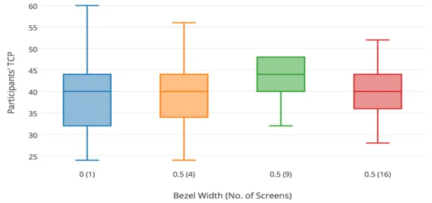
Figure 3.1: Tiled monitor configuration used in experiment [2x2]
• 4 x 4: This configuration has three horizontal and three vertical bezel rendered on screen. It is to simulate sixteen monitors joined together and making one large display.
The resultant resolution of each grid in the [2x2], the [3x3], and that [4x4] configurations is lower than that of real high resolution tiled monitor. Our findings are based on the replication of the real tiled monitors. The above four configuration with five bezel widths (0, 0.5, 1.0, 2.0, and 4.0cm) make a total of 13 tasks that each user suppose to do on a LC display.
The experimental design for this set up can be summarized as: 24 Participants x
13 Bezel Variations = 312 comparisons
Each participant received a random task out of 13 variations. The randomization in tasks shows the unbiased behaviour of the author towards the participants in the experiment.
3.2
Bezel width
In the first experiment we took four bezel widths: 0, 0.5cm, 1.0cm, 2.0cm, and in the second experiment we took a new bezel width of 4.0cm in addition to all the above. So, in total, five bezel widths were tested in the second experiment. According to a market survey, typically the available border width of an LC display for video wall is 2.0cm [56]. When two monitors are joined, the total width of the bezel is 4.0cm. Most of the tiled monitor displays available in market have less than 4.0cm bezel width. That is the reason we used a 2.0cm bezel width in the first experiment. The literature shows that experiments have been conducted with 0, 0.5, 1.0, 2.0 and 4.0cm bezel width to show how bezel width affects visual search and steering task [15, 56]. The quantity of data and the nature of the tasks that we used differentiate us from rest of the studies done in the past. There were 24 participants for each experiment and the experiments consisted of 10 and 13 tasks respectively. The puzzle-solving task involves the visual search for an image and placing the image at its specific location through navigation on the display. The tasks we have seen in the past research is either a directed task in which participants are directed to follow a path or to search for an object. In our experiments, participants locate an object and place it at its correct location. The order is randomized which means there is no unique image and there is no specific location. We designed the experiments according to the survey we did regarding the ratio of bezel width to display size.
3.3
Experimental task
The first experiment was a task in which participants were asked to solve a puzzle that poped up on a large display. The puzzle included the pictures of buildings from a local university. There were 13 pictures and they were totally randomized to maintain the un-biased nature of task.
The second experiment was exactly same as the first experiment, except that there was one more configuration of screen with bezel width of 4.0cm. Each experiment took approx-imately 30 minutes to complete all of its tasks. After the experiment, each participant was asked to fill a feedback form, which included a demographic questionnaire and questions about bezels.
3.4
Participants
Twenty four participants (nineteen men and five women) between the ages of 18 and 27 (median age 22) were recruited to participate in this study. Participants were Technology, Engineering, and Mathematics students who were enrolled at the University of Waterloo. Participants were daily computer users, and each has interacted with smart touch displays before. Each participant had either normal or corrected-to-normal vision and was right handed. Each participant was asked to sign an informed consent form. Upon arrival in the room, tasks were explained to participants, and they were allowed to get comfortable with the large display during a practice period for about 2-4 minutes. Practice period entailed the interaction with the display, solving an easy dummy puzzle, comfortably stand themselves in front of the display, signing a consent form. Each participant performed a puzzle solving task on a projected display approximately 200cm wide and 150cm tall. Each maintained a distance of approximately 40cm from the display which was at a resolution of 1980 x 1024 pixels on both the projector display and the LC display. See Figure 3.4.
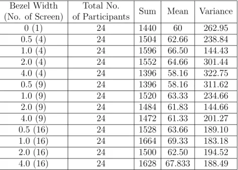
Each puzzle used in the experiments has 25 unsorted pieces and for every participant, a new puzzle popped up on the display. We measured each participant’s task completion percentage (TCP), which is defined as the number of pieces in an unsorted puzzle he or she managed to join correctly in the time of 120 seconds. If out of 25 pieces, a user manages to join 16 pieces correctly, then his TCP is 64%. After every task, the number of pieces joined correctly is noted down. Table 3.1 shows the combinations of tasks performed using the projector display. Table 3.2 shows the combinations using the LC display. Table 3.2 and Table3.1do not show the sequence of tasks performed because the sequence is randomized and it is different for every participant.
Figure 3.3: Tiled monitor configuration used in experiment [4x4]
3.5
Justification for the randomized behaviour of the
tasks
In the experiments, we randomly shuffled the images to generate a puzzle and each image is split into 25 equal sized pieces scattered on the display to generate a 5×5 matrix. A user is then required to solve the puzzle, i.e, to arrange the shuffled pieces of an image to its original position. We calculated the average of the times taken by the users to complete this task. When the tasks were distributed to the users, there were two options:
• The image is randomly shuffled once. Each user is given the same randomly shuffled image and then the average and other statistics are computed.
• The original image is randomly shuffled for each user. The drawback of this approach is that different users may get tasks of different difficulties.
In this thesis, we used the second approach for our experiments. Since each user solved a different task and then we computed the average statistics. We should justify why this approach makes sense. In our experiments, the users were required to arrange a 5×5 image. This was repeated for 24 users.
We modelled the task as follows. An image can be thought of as the vector V = (1, . . . ,25). We randomly permute the vector V to get a new vector V0. The task of the user is then to rearrangeV0 to get V. However, this arrangement can be done using only swap operations. The difficulty of this task can be measured by the number of swaps it takes to achieveV when we start from V0.
Difficulty(Task) = # Swaps to rearrange V0 to V.
To justify our experiment and show that our results are meaningful, we should show that on an average each user solved a task of similar difficulty. To verify this, we ran the following computer simulation.
• Generate a random permutation V0 of the vector V= (1, . . . ,25).
• Count the number of swaps needed to transform V0 to V.
• Repeat the above for 50 iterations and calculate the average and the standard devi-ation.
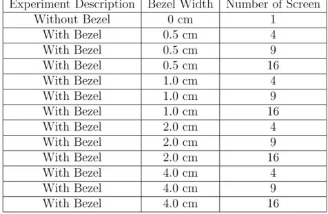
Experiment Description Bezel Width Number of Screen Without Bezel 0 cm 1 With Bezel 0.5 cm 4 With Bezel 0.5 cm 9 With Bezel 0.5 cm 16 With Bezel 1.0 cm 4 With Bezel 1.0 cm 9 With Bezel 1.0 cm 16 With Bezel 2.0 cm 4 With Bezel 2.0 cm 9 With Bezel 2.0 cm 16
Table 3.1: Design of Experiments - Projector Display
We ran the simulation and observed that the mean is∼21 and standard deviation of about ∼1.5. The small value of standard deviation shows that on an average each user solved a task of equal difficulty.
Before, we started the tasks, the touch screen was calibrated for each participant to maintain equality and to rectify errors. The hypotheses that were tested are:
• H10: User task performance is not affected by increasing the width of bezel. • H11: User task performance is affected by increasing the width of bezel.
• H20: User task performance is not affected by increasing the number of bezels. • H21: User task performance is affected by increasing the number of bezels.
Experiment Description Bezel Width Number of Screen Without Bezel 0 cm 1 With Bezel 0.5 cm 4 With Bezel 0.5 cm 9 With Bezel 0.5 cm 16 With Bezel 1.0 cm 4 With Bezel 1.0 cm 9 With Bezel 1.0 cm 16 With Bezel 2.0 cm 4 With Bezel 2.0 cm 9 With Bezel 2.0 cm 16 With Bezel 4.0 cm 4 With Bezel 4.0 cm 9 With Bezel 4.0 cm 16
Chapter 4
Results
This section discusses the results of the two experiments. Section4.1 discusses the results produced using the projector display. Section4.2 discusses the results produced using the LC display.
4.1
Projector display analysis
We did the experiment with 240 comparisons, arising from 10 experimental tasks x 24 participants. The TCP of the 24 participants for each task is shown in Table 4.1. First, we compare and analyze the whole experimental data and determine which hypotheses are supported. For each analysis, we use one-way ANOVA with anα-value of 0.05. The mean and variance of each task is shown in Table 4.2. Distribution of data is showed in box and whisker plot in Figure ??
Bezel Width (No. of Screens) Participants 1 2 3 4 5 6 7 8 9 10 11 12 13 14 15 16 17 18 19 20 21 22 23 24 0 (1) 36 32 44 24 40 32 52 36 32 60 32 52 44 36 48 44 44 48 44 36 32 40 32 40 0.5 (4) 40 32 40 36 40 36 40 56 44 32 36 48 32 40 32 44 44 48 40 24 32 40 52 44 1.0 (4) 38 40 40 44 32 44 56 44 32 32 36 44 52 44 52 44 48 52 36 52 60 44 28 36 2.0 (4) 44 32 48 32 32 28 44 48 32 36 40 56 40 40 36 40 48 52 40 28 40 40 48 44 0.5 (9) 44 48 40 48 36 44 48 32 40 44 44 48 40 36 32 48 48 40 40 48 48 48 44 48 1.0 (9) 44 48 40 36 32 44 60 40 36 32 36 48 48 48 48 44 40 36 36 52 32 44 48 40 2.0 (9) 44 32 40 40 40 48 32 28 48 40 44 44 40 36 36 36 48 40 48 40 40 40 40 52 0.5 (16) 32 40 40 36 40 48 32 36 36 52 40 48 40 48 40 52 44 44 36 44 36 36 44 28 1.0 (16) 40 60 44 36 36 48 44 36 36 32 40 48 40 48 28 44 48 40 40 44 32 36 44 44 2.0 (16) 36 36 44 40 44 40 44 40 44 52 48 48 52 44 36 52 48 44 40 40 38 44 32 36
Bezel Width (No. of Screen)
Total No.
of Participants Sum Mean Variance
0 (1) 24 960 40 69.56 0.5 (4) 24 952 39.66 52.75 1.0 (4) 24 1030 42.91 69.21 2.0 (4) 24 968 40.33 55.53 0.5 (9) 24 1036 43.16 27.79 1.0 (9) 24 1012 42.16 50.05 2.0 (9) 24 976 40.66 32.92 0.5 (16) 24 972 40.5 39.39 1.0 (16) 24 988 41.17 46.57 2.0 (16) 24 1022 42.58 30.77
Table 4.2: ANOVA Mean and Variance for complete data set Source of Variation SS df MS F P-value F crit
Between Groups 356.26 9 39.58 0.83 0.58 1.92 Within Groups 10915.67 230 47.45
Total 11271.93 239
Table 4.3: ANOVA Analysis for complete data set
There are two variable,bezel widthandnumber of screens1, which vary and are mutually exclusive. Tables4.2and4.3gives the mean andσof the complete data set and the ANOVA analysis of the same data set respectively. From the above analysis, the hypotheses might be supported or not, but concluding at this point is not justifiable until we go into details by fixing one variable out of the two. To make it more clear, we did several more analyses using the same data, but this time we fixed the number of screens and varied the bezel width. So, in total there are three data sets as shown in Table 4.4, 4.6, and 4.8.
In Tables 4.4 and 4.5, we fix the number of screens to be 4 and vary the width of a bezel to be 0.5cm, 1.0cm, and 2.0cm. The ANOVA shows that F2,69 = 1.1953, P −value = 0.3087, and Fcrit = 3.1296. Clearly, F2,69 ≺Fcrit, and P −value α, which mean that
there is no significant difference among the participants in their performance. Hence, the null hypothesisH10 is accepted, and its corresponding non-null hypothesisH11is rejected.
1Bezel width and number of bezels are the two variables mentioned in the hypotheses. An increase
in thenumber of screens results in an increase in thenumber of bezels. In order to make the discussion understandable, we will use thenumber of screens instead of the number of bezelsin this section.
Bezel Width (No. of Screen)
Total No.
of Participants Sum Mean Variance
0.5 (4) 24 952 39.66 52.75
1.0 (4) 24 1030 42.91 69.21
2.0 (4) 24 968 40.33 55.53
Table 4.4: Mean and Variance of data set keeping number of screens = 4 and varying width of Bezel
Source of Variation SS df MS F P-value F crit Between Groups 141.44 2 70.72 1.19 0.30 3.12
Within Groups 4082.5 69 59.16
Total 4223.94 71
Table 4.5: ANOVA Analysis of4.4
Therefore, we conclude that a user’s performance is not affected by variation in the bezel width.
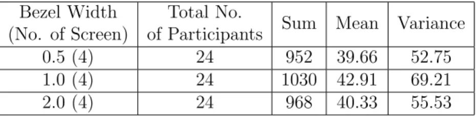
Bezel Width (No. of Screen)
Total No.
of Participants Sum Mean Variance
0.5 (9) 24 1036 43.16 27.79
1.0 (9) 24 1012 42.16 50.05
2.0 (9) 24 976 40.66 32.92
Table 4.6: Mean and Variance of data set keeping number of screens = 9 and varying width of Bezel
In Tables 4.6 and 4.7, we fix the number of screens to be 9 and vary the width of a bezel to be 0.5cm, 1.0cm, and 2.0cm. The ANOVA shows that F2,69 = 1.0290, P −value = 0.3627, and Fcrit = 3.1296. Clearly, F2,69 ≺Fcrit, and P −value α, which mean that there is no significant difference among the participants in their performance. Hence, the null hypothesis H10 is accepted, and its corresponding non-null hypothesisH11is rejected. Therefore, we conclude that a participant’s performance is not affected by variation in the bezel width.
In Tables 4.8 and 4.9, we fix the number of screens to be 16 and vary the width of a bezel to be 0.5cm, 1.0cm, and 2.0cm. The ANOVA shows that F2,69 = 0.6980, P −value = 0.5010, and Fcrit = 3.1296. Clearly, F2,69 ≺Fcrit, and P −value α, which mean that
Figure 4.1: Distribution of data set4.4 keeping the number of screens = 4 and varying the width of bezels
Figure 4.2: Distribution of data set4.6 keeping the number of screens = 9 and varying the width of bezels
Source of Variation SS df MS F P-value F crit
Between Groups 76 2 38 1.02 0.36 3.12
Within Groups 2548 69 36.92
Total 2624 71
Table 4.7: ANOVA Analysis of4.6
Bezel Width (No. of Screen)
Total No.
of Participants Sum Mean Variance
0.5 (16) 24 972 40.5 39.39
1.0 (16) 24 988 41.16 46.57
2.0 (16) 24 1022 42.58 30.78
Table 4.8: Mean and Variance of data set keeping number of screens = 16 and varying width of Bezel
null hypothesisH10 is accepted, and its corresponding non-null hypothesisH11is rejected. Therefore, we conclude that a participant’s performance is not affected by variation in the bezel width.
From the above discussions of Tables 4.5, 4.7, and 4.9, the null hypothesis H10 is accepted, that is, user task performance is not affected by increasing the width of bezels.
In the next discussion, we examine the data set in which we fix the bezel width to determine if there is any effect in a participant performance when we vary the number of screens as 1, 4, 9, and 16. An increase in the number of screens results in an increase in the number of bezels. In the discussion, we have Table 4.10, 4.12, and 4.14 with three different bezel widths, 0.5, 1.0, and 2.0, respectively.
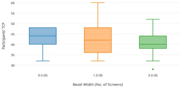
In Tables 4.10 and 4.11, we fix the bezel width to be 0.5cm and vary the number of screens to be 1, 4, 9, and 16. The ANOVA shows thatF3,92 = 1.2852,P −value= 0.2841, and Fcrit = 2.7035. Clearly, F3,92 ≺ Fcrit, and P −value α, which mean that there
is no significant difference among the participants in their performance. Hence, the null hypothesis H20 is accepted, and its corresponding non-null hypothesis H21 is rejected. Therefore, we conclude that a participant’s performance is not affected by variation in the number of screen.
In Tables 4.12 and 4.13, we fix the bezel width to be 1.0cm and vary the number of screens to be 1, 4, 9, and 16. The ANOVA shows that F3,92 = 0.6520,P −value= 0.5836, and Fcrit = 2.7035. Clearly, F3,92 ≺ Fcrit, and P −value α, which mean that there
Figure 4.3: Distribution of data set 4.8 keeping the number of screens = 16 and varying the width of bezels
Figure 4.4: Distribution of data set 4.10 keeping the width of the bezel = 0.5cms and varying the number of screens
Source of Variation SS df MS F P-value F crit Between Groups 54.33 2 27.16 0.69 0.50 3.12
Within Groups 2685.16 69 38.91
Total 2739.5 71
Table 4.9: ANOVA Analysis of4.8
Bezel Width (No. of Screen)
Total No.
of Participants Sum Mean Variance
0 (1) 24 960 40 69.56
0.5 (4) 24 952 39.66 52.75
0.5 (9) 24 1036 43.16 27.79
0.5 (16) 24 972 40.5 39.39
Table 4.10: Mean and Variance of data set keeping width of the Bezel = 0.5cms and varying number of screens
hypothesis H20 is accepted, and its corresponding non-null hypothesis H21 is rejected. Therefore, we conclude that a participant’s performance is not affected by variation in the number of screen.
In Tables 4.14 and 4.15, we fix the bezel width to be 2.0cm and vary the number of screens to be 1, 4, 9, and 16. The ANOVA shows that F3,92 = 0.6811,P −value= 0.5657, and Fcrit = 2.7035. Clearly, F3,92 ≺ Fcrit, and P −value α, which mean that there
is no significant difference among the participants in their performance. Hence, the null hypothesis H20 is accepted, and its corresponding non-null hypothesis H21 is rejected. Therefore, we conclude that a participant’s performance is not affected by variation in the number of screen.
From the above discussions of Tables 4.11, 4.13, and 4.15, the null hypothesis H20 is accepted, that is, user task performance is not affected by increasing the number of bezels.
4.2
LC display analysis
We did the experiment with 312 comparisons, arising from 13 experimental tasks x 24 participants. The task completion percentage (TCP) of 24 participants for each task is shown in Table 4.16. First, we compare and analyze the whole experimental data and
Figure 4.5: Distribution of data set 4.12 keeping the width of the bezel = 1.0cm and varying the number of screens
Figure 4.6: Distribution of data set 4.14 keeping the width of the bezel = 2.0cms and varying the number of screens
Source of Variation SS df MS F P-value F crit Between Groups 182.66 3 60.88 1.28 0.28 2.70
Within Groups 4358.66 92 47.37
Total 4541.33 95
Table 4.11: ANOVA Analysis of 4.10
Bezel Width (No. of Screen)
Total No.
of Participants Sum Mean Variance
0 (1) 24 960 40 69.56
1.0 (4) 24 1030 42.91 69.21
1.0 (9) 24 1012 42.16 50.05
1.0 (16) 24 988 41.16 46.57
Table 4.12: Mean and Variance of data set keeping width of the Bezel = 1.0cm and varying number of screens
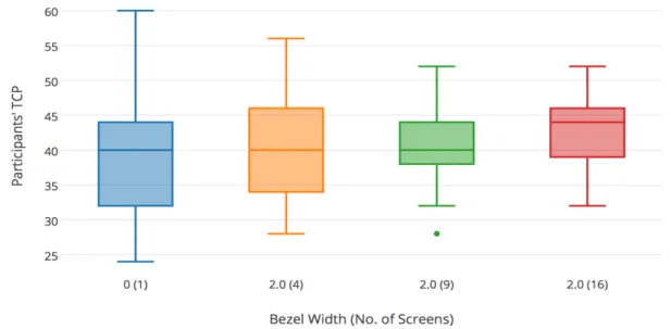
determine which hypotheses are supported. For each analysis, we use one-way ANOVA with an α-value of 0.05. The mean and variance of each task is shown in Table 4.17. Distribution of data is showed in box and whisker plot in Figure ??
There are two variable,bezel width andnumber of screens, which vary and are mutually exclusive. Tables 4.17 and 4.18 gives the Mean and σ of the complete data set and the ANOVA analysis of the same data set respectively. Similar to the discussion in Section4.1, we did several more analysis using the same data but first, we fix the number of screens and varied the bezel width. So, in total there are three sets as shown in Table 4.19 ,4.21, and 4.23.
Source of Variation SS df MS F P-value F crit Between Groups 115.125 3 38.37 0.65 0.58 2.70
Within Groups 5414.5 92 58.85 Total 5529.625 95
Table 4.13: ANOVA Analysis of 4.12
Bezel Width (No. of Screen)
Total No.
of Participants Sum Mean Variance
0 (1) 24 960 40 69.56
2.0 (4) 24 968 40.33 55.53
2.0 (9) 24 976 40.66 32.92
2.0 (16) 24 1022 42.58 30.77
Table 4.14: Mean and Variance of data set keeping width of the Bezel 2.0cms and varying number of screens
Source of Variation SS df MS F P-value F crit Between Groups 96.45 3 32.15 0.68 0.56 2.70
Within Groups 4342.5 92 47.20
Total 4438.95 95
Bezel Width (No. of Screens) Participants 1 2 3 4 5 6 7 8 9 10 11 12 13 14 15 16 17 18 19 20 21 22 23 24 0 (1) 48 48 72 60 76 44 72 52 80 64 44 72 44 40 72 60 64 72 32 76 24 72 68 84 0.5 (4) 84 64 64 76 64 20 60 52 64 72 52 20 72 64 68 64 68 72 64 72 76 72 72 48 1.0 (4) 56 56 84 72 76 60 48 60 72 84 72 60 68 68 72 64 68 76 28 72 72 76 60 72 2.0 (4) 84 60 52 84 84 64 28 84 84 64 72 84 40 68 44 68 72 76 52 68 60 68 24 68 4.0 (4) 84 64 48 76 16 48 56 64 36 84 68 84 36 72 60 72 40 76 44 44 56 56 40 72 0.5 (9) 84 84 48 40 64 16 40 72 84 52 44 52 52 72 64 72 52 84 48 40 60 60 40 72 1.0 (9) 60 60 72 84 80 40 32 68 64 84 56 44 56 72 68 84 60 84 60 56 52 40 60 84 2.0 (9) 64 72 68 48 76 52 48 68 48 60 60 48 64 60 76 84 60 80 40 60 64 48 56 80 4.0 (9) 84 60 56 56 64 40 48 52 76 84 44 80 72 56 48 76 64 80 60 64 64 32 64 48 0.5 (16) 80 48 60 40 64 48 64 80 60 76 84 48 36 68 48 80 68 84 60 72 72 60 68 60 1.0 (16) 60 60 80 72 84 68 60 68 48 84 84 68 64 84 60 76 72 80 72 76 68 24 72 80 2.0 (16) 84 72 52 52 60 84 56 52 64 64 68 72 40 76 72 76 36 84 44 56 68 68 44 56 4.0 (16) 68 80 84 84 56 64 48 68 80 84 64 76 60 64 68 68 48 84 64 64 84 28 68 72
Bezel Width (No. of Screen)
Total No.
of Participants Sum Mean Variance
0 (1) 24 1440 60 262.95 0.5 (4) 24 1504 62.66 238.84 1.0 (4) 24 1596 66.50 144.43 2.0 (4) 24 1552 64.66 301.44 4.0 (4) 24 1396 58.16 322.75 0.5 (9) 24 1396 58.16 311.62 1.0 (9) 24 1520 63.33 234.66 2.0 (9) 24 1484 61.83 144.66 4.0 (9) 24 1472 61.33 201.27 0.5 (16) 24 1528 63.66 189.10 1.0 (16) 24 1664 69.33 183.18 2.0 (16) 24 1500 62.50 194.52 4.0 (16) 24 1628 67.833 188.49
Table 4.17: ANOVA Mean and Variation for complete data sets Source of Variation SS df MS F P-value F crit
Between Groups 356.26 9 39.58 0.83 0.58 1.92 Within Groups 10915.67 230 47.45
Total 11271.93 239
Table 4.18: ANOVA Analysis for complete data set
In Tables 4.19 and 4.20, we fix the number of screens to be four and vary the width of a bezel to be 0.5cm, 1.0cm, 2.0cm, and 4.0cm. The ANOVA shows that F3,92 = 1.22,
P −value = 0.30, and Fcrit = 2.7. Clearly, F3,92 ≺ Fcrit, and P −value α, which
mean that there is no significant difference among the participants in their performance. Hence, the null hypothesisH10 is accepted, and its corresponding non-null hypothesisH11 is rejected. Therefore, we conclude that a participant’s performance is not affected by variation in the bezel width.
In Tables 4.21 and 4.22, we fix the number of screens to be nine and vary the width of a bezel to be 0.5cm, 1.0cm, 2.0cm, and 4.0cm. The ANOVA shows that F3,92 = 0.50,
P −value = 0.67, and Fcrit = 2.70. Clearly, F3,92 ≺ Fcrit, and P −value α, which
mean that there is no significant difference among the participants in their performance. Hence, the null hypothesisH10 is accepted, and its corresponding non-null hypothesisH11
Figure 4.7: Distribution of data set 4.19 keeping the number of screens = 4 and varying the width of bezels
Figure 4.8: Distribution of data set 4.21 keeping the number of screens = 9 and varying the width of bezels
Bezel Width (No. of Screen)
Total No.
of Participants Sum Mean Variance
0.5 (4) 24 1504 62.66 238.84
1.0 (4) 24 1596 66.50 144.43
2.0 (4) 24 1552 64.66 301.44
4.0 (4) 24 1396 58.16 322.75
Table 4.19: Mean and Variance of data set keeping number of screens = 4 and varying width of Bezel
Source of Variation SS df MS F P-value F crit
Between Groups 924 3 308 1.22 0.30 2.7
Within Groups 23172 92 251.86
Total 24096 95 I
Table 4.20: ANOVA Analysis of 4.19
is rejected. Therefore, we conclude that a participant’s performance is not affected by variation in the bezel width.
In Tables 4.23 and 4.24, we fix the number of screens to be 16 and vary the width of a bezel to be 0.5cm, 1.0cm, 2.0cm, and 4.0cm. The ANOVA shows that F3,92 = 1.35,
P −value = 0.26, and Fcrit = 2.70. Clearly, F3,92 ≺ Fcrit, and P −value α, which
mean that there is no significant difference among the participants in their performance. Hence, the null hypothesisH10 is accepted, and its corresponding non-null hypothesisH11 is rejected. Therefore, we conclude that a participant’s performance is not affected by variation in the bezel width.
From the above discussions of Tables 4.20, 4.22, and 4.24, the null hypothesis H10 is accepted, that is participant task performance is not affected by increasing the width of bezels.
In the next discussion, we examine the data set in which we fix the bezel width to determine if there is any effect in a participant performance when we vary the number of screens as 1, 4, 9, and 16. An increase in the number of screens results in an increase in the number of bezels. In the discussion, we have Table4.25, 4.27, 4.29, and4.31 with four different bezel widths, 0.5, 1.0, 2.0, and 4.0cm respectively.
In Tables 4.25 and 4.26, we fix the bezel width to be 0.5cm and vary the number of screens to be 1, 4, 9, and 16. The ANOVA shows that F3,92 = 0.60, P −value = 0.61, and Fcrit = 2.70. Clearly, F3,92 ≺ Fcrit, and P − value α, which mean that there is
Figure 4.9: Distribution of data set4.23 keeping the number of screens = 16 and varying the width of bezels
Figure 4.10: Distribution of data set 4.25 keeping the width of the Bezel = 0.5cms and varying the number of screens
Bezel Width (No. of Screen)
Total No.
of Participants Sum Mean Variance
0.5 (9) 24 1396 58.16 311.62
1.0 (9) 24 1520 63.33 234.66
2.0 (9) 24 1484 61.83 144.66
4.0 (9) 24 1472 61.33
Table 4.21: Mean and Variance of data set keeping number of screens = 9 and varying width of Bezel
Source of Variation SS df MS F P-value F crit Between Groups 340 3 113.33 0.50 0.67 2.7
Within Groups 20521.33 92 223.05 Total 20861.33 95
Table 4.22: ANOVA Analysis of 4.21
no significant difference among the participants in their performance. Hence, the null hypothesis H20 is accepted, and its corresponding non-null hypothesis H21 is rejected. Therefore, we conclude that a participant’s performance is not affected by variation in the number of screen.
In Tables 4.27 and 4.28, we fix the bezel width to be 1.0cm and vary the number of screens to be 1, 4, 9, and 16. The ANOVA shows that F3,92 = 1.88, P −value = 0.13, and Fcrit = 2.70. Clearly, F3,92 ≺ Fcrit, and P − value α, which mean that there is
no significant difference among the participants in their performance. Hence, the null hypothesis H20 is accepted, and its corresponding non-null hypothesis H21 is rejected. Therefore, we conclude that a participant’s performance is not affected by variation in the number of screen.
In Tables 4.29 and 4.30, we fix the bezel width to be 2.0cm and vary the number of screens to be 1, 4, 9, and 16. The ANOVA shows that F3,92 = 0.39, P −value = 0.75, and Fcrit = 2.70. Clearly, F3,92 ≺ Fcrit, and P − value α, which mean that there is
no significant difference among the participants in their performance. Hence, the null hypothesis H20 is accepted, and its corresponding non-null hypothesis H21 is rejected. Therefore, we conclude that a participant’s performance is not affected by variation in the number of screen.
In Tables 4.31 and 4.32, we fix the bezel width to be 4.0cm and vary the number of screens to be 1, 4, 9, and 16. The ANOVA shows that F3,92 = 1.74, P −value = 0.16,
Figure 4.11: Distribution of data set 4.27 keeping the width of the Bezel = 1.0cm and varying the number of screens
Figure 4.12: Distribution of data set 4.29 keeping the width of the Bezel = 2.0cms and varying the number of screens
Bezel Width (No. of Screen)
Total No.
of Participants Sum Mean Variance
0.5 (16) 24 1528 63.66 189.10
1.0 (16) 24 1664 69.33 183.18
2.0 (16) 24 1500 62.50 194.52
4.0 (16) 24 1628 67.833 188.49
Table 4.23: Mean and Variance of data set keeping number of screens = 16 and varying width of Bezel
Source of Variation SS df MS F P-value F crit Between Groups 769.33 3 256.44 1.35 0.26 2.70
Within Groups 17372 92 188.82 Total 18141.33 95
Table 4.24: ANOVA Analysis of 4.23
and Fcrit = 2.70. Clearly, F3,92 ≺ Fcrit, and P − value α, which mean that there is
no significant difference among the participants in their performance. Hence, the null hypothesis H20 is accepted, and its corresponding non-null hypothesis H21 is rejected. Therefore, we conclude that a participant’s performance is not affected by variation in the number of screen.
From the above discussions of Tables4.26,4.28,4.30, and4.32 the null hypothesisH20 is accepted, that is participant task performance is not affected by increasing the number of bezels.
We introduced the new bezel width of 4.0 cm in the LC display. The analysis showed that its behaviour is similar to that of the other bezel width. That is, H20 is accepted and
H21 is rejected. Combining the analyses of projector displays and LC displays, we reach the following results:
• A user’s performance is not affected by increasing the bezel width. • A user’s performance is not affected by increasing the number of bezels.
Bezel Width (No. of Screen)
Total No.
of Participants Sum Mean Variance
0 (1) 24 1440 60 262.95
0.5 (4) 24 1504 62.66 238.84
0.5 (9) 24 1396 58.16 311.62
0.5 (16) 24 1528 63.66 189.10
Table 4.25: Mean and Variance of data set keeping width of the Bezel = 0.5 cms and varying number of screens
Source of Variation SS df MS F P-value F crit Between Groups 452.50 3 150.833 0.60 0.61 2.7 Within Groups 23058 92 250.63
Total 23510.50 95
Table 4.26: ANOVA Analysis of 4.25
4.3
LC display versus projector display
We analyzed both projector display and LC display, considering a participant performance as the important parameters. We know that a projector display can produce an image which is free from bezel, and this cannot be achieved completely in a LC display. The best that we can have in a LC display is a very thin bezel, but such display are on the expensive side. In addition to bezel interference, there are other factors such as brightness, contrast, calibration, colour and resolution. The effort to calibrate a LC display is lower than calibrating a projector display. Although we keep brightness, contrast, resolution, and colour of both displays the same in the experiments, the display created with a projector appears to be different from a LC display. The projector display has slightly different colour range because of the bulb and colour filter [52]. The projector does not illuminate the screen uniformly, and that is why the projector display is slightly different from the LC display. It is difficult to come to conclusion that one display is better than other with the data we have, but we try to give a direction for future research. We take a LC display and projector display without bezel for the data analysis of this experiment. We use the same data that we gather for bezel width and utilize it towards a new aspect which is: a LC display is better than a projector displays when a single participant interacts with it.
Figure 4.14, the X-axis is the number of participants perform an experiment and the Y-axis is the task completion percentage. The graph shows the variation in task completion percentage of the LC display and the projector display of 24 participants. For 83.3% of the
Figure 4.13: Distribution of data set 4.31 keeping the width of the Bezel = 4.0cms and varying the number of screens
Bezel Width (No. of Screen)
Total No.
of Participants Sum Mean Variance
0 (1) 24 1440 60 262.95
1.0 (4) 24 1596 66.5 144.43
1.0 (9) 24 1520 63.33 234.66
1.0 (16) 24 1664 69.33 183.18
Table 4.27: Mean and Variance of data set keeping width of the Bezel = 1.0 cms and varying number of screens
Source of Variation SS df MS F P-value F crit Between Groups 1167.16 3 389.05 1.88 0.13 2.7 Within Groups 18980.67 92 206.31
Total 20147.83 95
Table 4.28: ANOVA Analysis of 4.27
participants, the TCP for the LC display is more than for the projector display. It is clear from the above evidence that with LC displays, participants are more comfortable than with projector displays. Every participant exceptparticipant 11, 13,19 and 21 shows more completion with LC displays. It is clearly visible that the average of 24 participants with the LC display average of 24 participants with the projector display, and it is because of the factors such as brightness, colour contrast, attractiveness of the display, aesthetics of the displays, among others, as we observed in feedback. Some participants are more comfortable with the greater brightness that a LC display has. On the contrary, a smaller number of them said that the LC display’s brightness is too high. So, talking about the other factors at this point will not take us anywhere unless we do the experiments by taking individual factors into account and focussing on one at a time. We leave that for future work. We do another analysis by plotting a graph with the data from Table 4.2
and 4.17. We plot the mean of every task performed by each participant with the LC display and the projector display. We eliminate the bezel width 4.0 cm for this analysis because this bezel width is not present in projector display. In the analysis, we are trying to determine the effect of the projector display and the LC display on the participants. So, for this analysis, we eliminate the effect of bezel width, as this is the common factor in both displays. Technically, participants did 10 tasks under the influence of the same factors such as variation in bezel width andnumber of bezels with the different displays. We can ignore the effect of variation in bezel width and number of bezels because their variation is the same in both experiments. From the Figure 4.15, in all the cases, participants are more
Bezel Width (No. of Screen)
Total No.
of Participants Sum Mean Variance
0 (1) 24 1440 60 262.95
2.0 (4) 24 1552 64.66 301.44
2.0 (9) 24 1484 61.83 144.66
2.0 (16) 24 1500 62.50 194.52
Table 4.29: Mean and Variance of data set keeping width of the Bezel = 2.0 cms and varying number of screens
Source of Variation SS df MS F P-value F crit Between Groups 267.33 3 89.11 0.39 0.75 2.70 Within Groups 20782.67 92 225.89
Total 21050 95
Table 4.30: ANOVA Analysis of 4.29
efficient with the LC display than with the projector display. In all 10 task variations, the mean for the LC display mean for the projector display. Hence, participants are more comfortable with a LC display than with a projector display under certain conditions.
Bezel Width (No. of Screen)
Total No.
of Participants Sum Mean Variance
0 (1) 24 1440 60 262.95
4.0 (4) 24 1396 58.166 322.75
4.0 (9) 24 1472 61.33 201.27
4.0 (16) 24 1628 67.83 188.49
Table 4.31: Mean and Variance of data set keeping width of the Bezel = 4.0 cms and varying number of screens
Source of Variation SS df MS F P-value F crit Between Groups 1273.33 3 424.44 1.74 0.16 2.70 Within Groups 22436 92 243.86
Total 23709.33 95
Table 4.32: ANOVA Analysis of 4.31
Chapter 5
Discussion
The data that we collected during the experiments help us to quantify the impact of bezel width and the number of bezels on user performance. Our null hypotheses H10 and H20 are supported. Thus the user is not affected by the bezel width and the number of bezels. Our results are aligned with those of the study conducted by Wallace et al. in which they show that bezels have no effect in visual task performance [56]. Some users in their feedback mentioned that the bezels seemed to be an obstacle. However, when we quantified the results, we did not find any problems caused by the bezel. It is plausible that users are expecting a delay in performance from the bezels, but when they actually performed on a large display, there was not any.
<

![Figure 3.1: Tiled monitor configuration used in experiment [2x2]](https://thumb-us.123doks.com/thumbv2/123dok_us/812432.2602725/28.918.149.788.194.536/figure-tiled-monitor-configuration-used-experiment-x.webp)
![Figure 3.3: Tiled monitor configuration used in experiment [4x4]](https://thumb-us.123doks.com/thumbv2/123dok_us/812432.2602725/31.918.149.785.194.536/figure-tiled-monitor-configuration-used-experiment-x.webp)