Public Investment and Re-election Prospects in Developed Countries

(1)

Public Investment and Re-election Prospects

in Developed Countries

Margarita Katsimi

Vassilis Sarantides

CES

IFO

W

ORKING

P

APER

N

O

.

3570

C

ATEGORY

2:

P

UBLIC

C

HOICE

S

EPTEMBER

2011

An electronic version of the paper may be downloaded

• from the SSRN website: www.SSRN.com

• from the RePEc website: www.RePEc.org

(2)

CESifo Working Paper No. 3570

Public Investment and Re-election Prospects

in Developed Countries

Abstract

A growing literature suggests that office motivated politicians manipulate fiscal policy instruments in order to seek their re-election. This paper investigates the impact of electoral manipulation of the level and composition of fiscal policy on incumbent’s re-election prospects. This impact is estimated for a panel of 21 OECD countries over the period 1972- 1999. Our results suggest that increased public investment during the term in office, as well as a shift in expenditures towards public investment can improve re-election prospects. On the contrary, election year manipulation via public investment does not affect re-election prospects. We also find that voters punish politicians who create deficits during elections, while deficits that proceed the election year have similar, although smaller effects on the reelection prospects.

JEL-Code: D720, E620.

Keywords: political budget cycles, elections, quality of public expenditure, public investment.

Margarita Katsimi

Athens University of Economics and Business / Department of International and

European Economic Studies Patision Str. 76 Greece – Athens 10434

mkatsimi@aueb.gr

Vassilis Sarantides

Athens University of Economics and Business / Department of International and

European Economic Studies Patision Str. 76 Greece – Athens 10434

sarantides@aueb.gr

August 2011

Without implicating, we wish to thank Simon Schnyder, Grigorios Siourounis and participants in seminars at the Athens University of Economics and Business and the 2011 European Public Choice Society conference. The usual disclaimer applies.

(3)

1. Introduction

Since Nordhaus (1975) seminal work, a rich literature suggests that office motivated incumbents apply expansionary fiscal policy in order to seek their re-election. In a rational expectations framework political budget cycles still arise under the driving assumption of temporary information asymmetries between voters and politicians regarding the competence level of the latter.1

Electoral manipulation of fiscal policy may also concern the composition of public spending rather than its level. Rogoff (1990) provided a firm theoretical foundation showing that electorally motivated incumbents signal their competence by shifting public spending towards more ‘visible’ government consumption and away from public investment goods. Following this argument Katsimi and Sarantides (2011) investigate the electoral impact on the composition of fiscal policy for a sample of developed countries.2 Their evidence suggest that during elections incumbents decrease capital expenditures as a percentage of GDP shifting the composition of public spending towards ‘visible’ current expenditures and away from capital expenditures. In addition, it seems that incumbents decrease public investment in order to finance a fall in direct taxation that provides an immediate economic benefit to voters while keeping the fiscal balance unaffected.

To what extend is, however, fiscal manipulation ‘punished’ by voters? In other words, does, fiscal manipulation affect the re-election probability, and if yes, is the effect positive or negative? To our knowledge, Brender and Drazen (2008) is the only existing study that directly tests at the national level the impact of budget deficits on the re-election probability.3 Their study finds no evidence that deficits help re-election, while in developed countries and in old democracies increased deficits reduce the probability of re-election. Other studies, conducted at state and local level in a single country, found that voters punish rather than reward loose fiscal policies (see Peltzman (1992), Brender (2003), Drazen and Elsava (2010)). These results support the notion that voters punish loose fiscal policies at the polls, and even more if they are perceived as electorally motivated.

Regarding the relationship between public investment expenditures and re-election prospects, studies are limited and are concentrated at the local level. Veiga and Veiga (2007) using a data set for Portuguese mainland municipalities for the period 1979-2001 find that

1

In the moral-hazard type political budget cycles (PBC) models the incumbent has an incentive to signal its level of competence by increasing election-year deficits, through expansion in expenditures or cuts in taxes, in order to provide immediate economic benefit to voters (see e.g. Rogoff and Sibert (1988)). On the other hand, in the adverse selection type PBC models (see e.g. Shi and Svensson (2006)) fiscal manipulation in equilibrium does not affect re-election probability.

2

For an empirical investigation of this argument for developing countries see Vergne (2009).

3

Buti et al. (2010) check the effect of economic reforms on re-election for a sample of 21 OECD countries over the period 1985-2003. They found that the electoral impact of the reform depends strongly on which types of policies are considered.

(4)

higher investment expenditures around elections, as well as during the term in office, are associated with a higher vote share for incumbent mayors.4 Sakurai and Menezes (2008) using a panel of more than 2000 Brazilian municipalities over the period 1988 to 2000, find that higher capital spending over the years preceding elections increase the re-election prospects, while the deviation of capital spending in election year is not beneficial to incumbent mayors.

In this study we attempt to bridge a gap in the literature by examining at the national level the impact of public investment and the composition of public spending on the incumbent’s re-election prospects. We believe that this is an important step in order to be able to derive more general policy conclusions since it is difficult to compare results applying to local governments across countries. This difficulty stems from the fact that fiscal items that are clearly identifiable as provincial government responsibilities differ from one country to another. In our analysis, distinguish between policies that occur in the election year and policies that occur proceeding the election year. Brender and Drazen (2008) found that in developed countries deficits in the earlier years of an incumbent’s term in office reduce the probability of re-election but to a less extent in comparison with election year deficits. Accordingly, we may anticipate that increased capital expenditures in the earlier years in office are better noticed by voters near the completion of the term, since these expenditures are mostly long term projects which are observed by voters with a lag.

To model the re-election determinants we use information on 122 electoral campaigns for 21 high-income OECD. Our empirical results suggest that re-election prospects improve following a rise in capital expenditures or a shift of expenditures towards capital expenditures during the incumbent’s term in office, while they remain unaffected by manipulation around the election period. Thus, although voters reward incumbents who promote public investment during their term in office, electoral spending on public investment is not rewarded. Similarly, a fall in public investment spending is not punished by voters. The latter can probably be attributed to the “lower visibility” of capital expenditures that are mostly long-term projects that increase voter’s utility upon completion (e.g. infrastructure) and are observed by the voters with a lag. Moreover, similarly to Brender and Drazen (2008) we find that voters in developed countries dislike and punish deficits and inflation.

4

It is worth noting that Adit et al. (2011) using the same sample of Portuguese municipalities show that opportunistic behavior of incumbent mayors leads to a higher win margin and that incumbents behave more opportunistically when their win margin is small.

(5)

The remainder of the paper is organized as follows. Section 2 describes the data, specifies the econometric model and contains our basic findings. Section 3 then reports the results of robustness tests. The last section concludes.

2. Econometric Analysis

2.1. Data and estimation method

The baseline political variable leader re-election is based on information from the “World Statesmen” encyclopedia and from the "Inter-Parliamentary Union" database. These data allow us to follows the terms of individual leaders and parties in office from appointment to termination, and to associate them with election dates. It is worth noting that we only include legislative elections for countries with parliamentary political systems and presidential elections for countries with presidential systems.

In line with Brender and Drazen (2008), leader re-election variable includes observations in which the leader has been in office for at least two years prior to the elections. It takes value 1 if the incumbent chief executive is re-elected and 0 otherwise. It also allows for the following special cases:

(i) In cases where the leader quits within the year of elections, leader re-election receives the value 0.

(ii)In cases where candidates replace leaders that were subject to a legal limit, leader re-election receives the value 1 if the reigning leader’s party is winning in the elections and 0 if it loses.

(iii) In cases where during the election year a leader is replaced because he died or quitted due to health problems, leader re-election receives the value 1 if the successor leader gets reelected and 0 otherwise.

(iv) If the appointed prime minister of the governing coalition after the current elections comes from the same party with his predecessor and this party received a higher support in comparison with previous election, leader re-election variable receives the value 1 and 0 otherwise. 5

Our sample includes 21 high-income OECD countries.6 Regarding the leader re-election

definition, we have 113 campaigns in which the leader was reelected in 57 cases. It is worth

5_{Becuase we do not want to reduce an already small sample, for special cases (ii) and (iv) we actually follow party’s}

re-election instead of leader re-re-election. Alternaltively, if we drop these observations from our sample qualitative results remain unaffected.

6

The countries of our sample are Australia, Austria, Belgium, Canada, Denmark, Finland, France, Germany, Greece, Iceland, Ireland, Italy, Japan, Luxemburg, Netherlands, Norway, Portugal, Spain, Sweden, United Kingdom and United States. South Korea is excluded from the sample because the President has no possibility of re-election, while at the same

(6)

noting that in 109 out of 113 campaigns of our sample the same person who had been the head of the government before the elections is the one seeking for re-election.

Following previous studies in this area our empirical analysis is based on central government data [see among others, Schuknecht (2000) and Brender and Drazen (2008)]7. Our fiscal data are obtained from the Global Development Network Growth Database (GDNGD). Primary data for the proceeds are taken from IMF, "Government Financial Statistics" (GFS); and data for GDP come from Global Development Finance and World Development Indicators. Note that due to data availability we have to restrict our data set to the period from 1972 to 1999.8 A complete list of all variables used in our estimations is provided in the Data Appendix with details on data sources and descriptive statistics.

In order to model the impact of public investment on re-election prospects, we use the economic classification provided by the GFS database and we construct variable capital term

by computing the average of the capital expenditures during the leader’s current term in the office (excluding the election year of previous elections, but including the election year of current elections). At the same time, we want to check if pre-electoral manipulation in capital expenditures affects re-election prospects. For this reason we split variable capital term into variables capital deviation and capital non-election. The first of these two variables is the change in the capital expenditures in the election year relative to the average of the years preceding elections (excluding the election year of previous elections). The second of these two variables is the average in the fiscal variable during the leader’s (party’s) term in the office preceding the election year (excluding the election year of previous elections). Finally, given that it takes time for investment to be materialized, we include in our estimations variable initial capital, which is capital expenditures as a percentage of GDP in the first year during the term in office (we do not consider in the term the election year of previous elections).

Alternatively, we calculate the percentage of central government’s capital to current expenditures in order to test if the composition of expenditures affects re-election prospects.

time we cannot follow party’s re-election for the two observations we have (1992, 1997) since they were dissolved. New Zealand is excluded from the sample due to unavailability for fiscal data. We included in the sample two small OECD countries Iceland and Luxemburg because we did not want to reduce an already small sample. Moreover, when we dropped these countries from our sample qualitative results remain unaffected.

7

We base our analysis on central government data for two reasons: First, given that general government data include all levels of

government (state, local, central), results based on such data would be more difficult to interpret. As noted by Schuknecht (2000) the central government controls directly only its own budget while changes in public spending of the general government may be affected by both state and local elections. Second, data from general government accounts are less consistent across countries and time periods.

8

GFS data until the late nineties has been calculated using Government Finance Statistics Manual 1986 classification, while data beyond this point has been calculated with the Government Finance Statistics Manual 2001 framework. Unfortunately, the new classification does no longer provide data for the capital expenditures and current expenditures series included in the GFSM 1986 classification. For more details see Katsimi and Sarantides (2011).

(7)

In a direct analogy to the definitions in the previous paragraph regarding capital expenditures, we construct variables composition term, composition deviation, composition non-election

and initial composition.

Apart from the fiscal variables, we include in our estimated model a number of socio-economic and political variables. More specifically the following control variables are included in the model specification:

(i) Macroeconomic conditions: For comparison reasons we use the main control

variables of Brender and Drazen (2008) namely the growth rate of output (growth term) and the inflation rate (inflation term) during the term in office. Although studies for developed countries contradict regarding the effect of growth rates of output on voting behavior (see e.g. Brender and Drazen (2008), Alesina and Rosenthal (1995)), we anticipate that a higher growth rate during the term in office is positively associated with re-election prospects. On the contrary, we expect that variable inflation term affects negatively re-election prospects since voters dislike inflation and punish at the polls incumbents that create it (see e.g. Alesina et al. (1998)). These data are from the World Bank's ‘World Development Indicators’ (WDI).

(ii)New democracy effect: We include in our estimations the dummy variable new democracy that receives the value 1 for the period of the first 4 elections after Greece, Portugal and Spain shift to a democratic regime. According to Brender and Drazen (2005), these “new” democracies are more prone to fiscal manipulation, since incumbents might be rewarded at the polls if they can “mislead” inexperienced voters by attributing the good economic conditions to their competency.9

(iii)Level of “awareness”: As a measure of “awareness” we use variable illiteracy term

that is the proportion of population aged 15 years old and above with no schooling. It is taken by a dataset collected by Barro and Lee (2010) that covers successive five year averages. We expect illiteracy rate to be associated with low levels of voter “sophistication” and, hence, with higher re-election prospects.

(iv)Ideological orientation: We create dummy variable centre (left) that receives the value 1 if the cabinet in power scores 3 (4 or 5) on the ideology index govparty of Armigneon et al. (2008). We expect that the probability of success is much lower for centrist governments since these governments are in most of the cases coalition and

9

We included in our sample Greece, Portugal and Spain, because we did not want to reduce an already small sample. On the other hand, when we drop from our estimations these countries our qualitative results remain unaffected.

(8)

fragmented governments.10 At the same time, we want to test for differences in re-election prospects between left-wing and right wing incumbents.

(v) Reforms: Finally, we include in our estimations dummy variable EU that receives the value 1 for the period 1993-1999 for countries that where members of the European Union and signed the Maastricht treaty. This variable receives the value 1 for the period 1995-1999 for Austria, Finland and Sweden that become members of the European Union at the 1 January 1995. Note that the period after the adjustment of ERM bands and before the establishment of the euro-area was characterized by EU member states effort to comply with the convergence criteria. This effort included a process for fiscal consolidation. Thus, this variable should capture the impact of the countries effort to adopt the Euro on the incumbent’s re-election prospects.

It is also worth mentioning, that we have attempted to include in our model a series of other control variables such as the percentage of votes the incumbent receive in the previous elections, dummies to control for majoritarian vs. proportional systems and presidential vs. parliamentary governments as well the number of terms the incumbent chief executive has been in office. However, none of these variables had a significant effect on re-election prospects and in order to preserve degrees of freedom we do not include them in our estimations.11

We examine the impact of fiscal performance on re-election prospects using a Probit estimator with robust standard errors to both heteroskedasticity (Huber-White sandwich estimators) and any form of intra-cluster serial correlation.12 It is worth noting that we test for the presence of random effects using a likelihood ratio test. According to the results we cannot reject the null hypothesis that all slope coefficients are simultaneously equal to zero and consequently that random effects improve the pooled model significantly. In our panel where the number of cross sections exceeds the number of time units, the pooled Probit model would be more efficient since it requires fewer parameters to be estimated in comparison with a random effects model.13

10

We also included in the model specification a dummy variable that receives the value of 1 for coalition governments and 0 otherwise. In accordance with the findings of Alesina et al. (1997) we find a negative relation between coalition governments and the probability of re-election. At the same time, when we inserted in our regressions cabinet orientation, the coefficient for coalition governments turned out insignificant, while results for all other variables remain unchanged. This is a clear indication that centre orientated governments and coalition governments are two sides of the same coin.

11_{Note that including these additional control variables in our specification does not change our basic findings. Results}

available upon request.

12

We also repeat the same estimations using a Logit specification without any qualitative change in our results.

13

It is worth noting that if we account for heterogeneity among countries using a Random Effects model, qualitative results (available upon request) do not change significantly. On the other hand, we have not attempted to apply Fixed Effects in our Probit regressions, because this would lead to inconsistent estimates (see e.g. Woolridge (2002))

(9)

2.2. Results

In Table 1 we examine the effect of capital expenditures and the composition of public expenditures on the probability of re-election. Regarding the socio-economic variables, we observe that inflation term is negative and statistically significant, while growth term is insignificantly related with leader re-election. These results seem to verify the previous studies of Alesina et al. (1998) and Brender and Drazen (2008) who found that voters dislike inflation, while growth rate does not seem to affect re-election prospects. Moreover, the coefficient of variable illiteracy term is positive and statistically significant, indicating that lower levels of voter awareness are positively related to reelection prospects.

Regarding government’s ideology, our results indicate that variable left (centre) is positive (negative) and significantly related with leader re-election. These results show that leftist (centrist) governments seem to have a higher (lower) probability to get re-elected in comparison with right wing governments. This result could reflect that more often leftish incumbents adopt policies that are more ‘popular’ to the majority of voters. As far as the centrist incumbents are concerned, this result might be related to the fact that centrist governments are in most of the cases fragmented coalition governments. In addition, variable new democracy is positive when statistically significant, indicating that in new democracies leaders have a higher probability to get re-elected. Finally, variable EU has a negative and significant coefficient in all estimated equations. This result could be attributed to the conduct of strict and ‘unpopular’ policies aiming at that the nominal convergence process required by euro-area participation.

Table 1 here

Regarding the fiscal performance, as can be seen in column 1 (4) of Table 1 we show that variable capital term (composition term) is positively and significantly related to leader re-election at the 1% (5%) level of significance. This result indicates an increase of 1% in

capital term (composition term) leads to an increase of about 9.4% (3.3%) in the chances of re-election.

As a next step, we split variables capital and composition term into variables capital deviation and capital non-election and variables composition deviation and composition non-election. As can be seen in columns 2 and 5 respectively, variables capital deviation and

(10)

to the average of the years preceding elections (excluding the election year of previous elections), do not seem to affect re-election prospects. Existing empirical evidence for the same sample of countries suggests that during elections capital expenditures decrease in order to finance a fall in direct taxation [see Katsimi and Sarantides (2011)]. This finding simply indicates that this fall in capital expenditure is not ‘punished’ by voting behaviour because this cut is not ‘visible’ by voters in the election period. Capital expenditures (e.g. infrastructure) are mostly long-term projects that will increase voter’s utility upon completion. Likewise, a change in the expenditure composition initiated by the fall in capital expenditure does not affect voting behaviour because this cut is not ‘visible’ in the election period. On the contrary, variables capital non-election and composition non-election over the term in office, excluding the election year, are positive and significantly related to leader re-election. More specifically, an increase of 1% in capital non-election (composition non-election) can increase the probability of re-election by 10.4% (3.4%). Finally, in columns 3 and 6 we observe that variables initial capital and composition are positively related to leader re-election. As expected, given that it takes time for investment to be materialized, capital expenditures in the first year of the term in office are most likely to be visible to voters at the election period increasing the re-election prospects of the incumbent. In particular, an increase of 1% in initial capital (initial composition) leads to an increase of about 8.7% (3.0%) in the chances of re-election. This implies that an incumbent who wishes to maximize his re-election prospects should frontload public spending: He should spend on capital as soon as he is elected in order to allow for a sufficient period for this spending to be materialized and observed by voters while he should lower capital spending in the final year of his term when this type of spending has the lowest visibility.

3. Robustness

In this section we examine the robustness of the above results by re-estimating our regressions under various modifications. First, we check if our results remain unaffected when we keep in regressions only the predetermined elections. Second, we create variable

party re-election so that to associate election outcomes with party’s performance. Finally, we add in our estimations fiscal variables surplus and revenues in order to have a complete specification of the budget constraint.

(11)

Regarding the timing of elections, Katsimi and Sarntides (2011) found that only during

predetermined elections incumbents reduce capital expenditures and shift the composition of expenditures towards public investment. This result is consistent with Roggof’s (1990) argument that during predetermined elections opportunistic incumbents have ample to use fiscal policy in order to increase re-election probabilities, far greater, compared to the case of elections being called earlier. Hence, in line with Brender and Drazen (2005) we look at the constitutionally-determined election interval and we keep in or sample those elections that are characterized as predetermined and are held during the expected year of the constitutionally-fixed term. At the same time we choose to exclude endogenous elections from our sample since they probably introduce an important endogeneity bias. In endogenous elections the re-election probability can affect the re-election date in two ways: Firstly, re-elections may be called when the re-election prospects are favourable and secondly, coalition governments may be more vulnerable when re-election probability is low. As can be seen in Table 2, our results indicate that excluding endogenous elections suggests an even stronger connection between the fiscal variables and re-election prospects. For instance, we observe that an increase of 1% in capital term (composition term) leads to an increase of about 16.5% (4.5%) in the chances of re-election.

Table 2 here

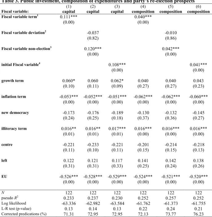
3.2. Party vs. leader re-election

Until now we have applied as dependent variable in our estimations leader re-election that follows the terms of individual leaders in office. Given that parties stay in power for longer periods than leaders and that capital expenditure are mostly long-term projects that will increase voter’s utility upon completion, one could expect investment expenditures to have a stronger impact on parties’ re-election than on leaders’ re-election. Hence, in accordance to the construction of variable leader re-election we alternatively follow the terms of parties in office and we construct variable party re-election. It should be mentioned that we have many cases in our sample in which the values of the two key political variables deviate. For instance, when the leader in office resigns within the year of election variable leader re-lection receives value 0, while party re-election receives value 1 if the successor leader comes from the same party and gets reelected. Regarding the party re-election definition, we have 122 campaigns in which the party in power was reelected in 71 cases. As expected, in Table 3, we depict an even stronger relationship between public investment and the

(12)

composition of expenditures to party re-election. Hence, we find that an increase of 1% in

capital term (composition term) leads to an increase of about 11.1% (4.0%) in the chances of re-election.

Table 3 here

3.3. Additional fiscal instruments

The final robustness exercise we conduct is to add budget surplus/deficit and total revenues in our estimations in order to have a full specification of the government budget constraint [see Kneller et al. (1999)].14 In order to avoid perfect multi-collinearity one element of the government budget should be omitted. Given that in columns 4 to 6 of Table 4 we include variable composition term that contains variable current expenditures, we choose to omit the latter from the specification. Regarding the interpretation of the results, the estimated coefficient γj measures the marginal impact of fiscal variable Xj on re-election prospects, net

of the marginal impact of fiscal variable Xm, that we exclude from specification and is the

assumed financing element. This implies that current expenditures are the financing element in columns 1 to 3 and total expenditures in columns 3 to 6.

In accordance to the above definitions we construct for budget surplus/deficit variables surplus term, surplus deviation, surplus non-election and initial surplus, while similarly for total revenues we construct variables revenues term, revenues deviation,

revenues non-election and initial revenues. As can be seen in Table 3, total revenues do not seem to affect re-election chances in none of our estimations. On the contrary, in columns 1 to 3 we observe that except for the case of the first year during the term in office, budget surplus/deficit is rewarded/punished by the voters at the polls. In particular, a decrease of 1% in surplus term (surplus non-election) leads to a decrease of about 3.5% (4.8%) in the chances of re-election. In addition, it seems that election year deficits have an even stronger effect on the probability of re-lection. We find that a decrease of 1% in surplus deviation can decrease re-election chances by 7.9%. These findings are corroborated by the results presented in Brender and Drazen (2008), in which a decrease of 1% in the budget surplus deteriorates the probability of re-election by 3 to 5% in developed countries and that a decrease of 1% in the surplus during an election year decreases the probability of re-election by 7 to 9%. Based on the full specification of the government budget constraint we have

(13)

implemented, this implies that if the incumbent increase the budget deficit around elections via current expenditures this will decrease the chances of re-election by 7.9%. This implies that incumbents have an incentive to avoid deficit creation and to finance expansionary fiscal policies through a fall in less visible capital spending. Regarding capital expenditures, we find that decreasing public spending in the election year is not ‘punished’ by voters, while overall public investment spending has a positive impact on the incumbent’s probability of re-election. This is an expected result, since it is logical to assume that overall public investment spending is more visible to voters than capital spending in the election period.

Table 4 here

Next, in columns 3 to 6 we observe that election year deficits seem to decrease the probability of re-election by 7.6%, while deficits over the term in office and preceding the election year affect re-election prospects by 2.6% and 3.2% respectively. Given that we control for the composition of expenditures, this means that the probability of re-election deteriorates if incumbents increase the deficit over their term in office by increasing in equal proportions public investment and consumption. Finally, regarding the effect of the composition of expenditures on re-election prospects the qualitative results presented in Table 4 remain essentially the same as those depicted in Table 1.

4. Conclusions

This paper aims at investigating whether electoral manipulation of the level and the composition of fiscal policy can affect election prospects. We find evidence that re-election prospects improve following a rise in capital expenditures or a shift of expenditures towards capital expenditures during the term in office, while remain unaffected by manipulation around elections. One possible explanation is that election year manipulation in capital expenditures does not affect the probability of re-election due to “low visibility” of this type of expenditures. Capital expenditures (e.g. infrastructure) are mostly long-term projects that will increase voters’ utility upon completion. For that reason, capital spending at the beginning of the incumbent’s term in office has a positive impact on re-election prospects since it allows for a sufficient period in order for this spending to be observed by voters before elections. Finally, we have indications similar to those obtained by Brender and Drazen (2008), namely that voters in developed countries dislike and punish at the polls deficits and inflation.

(14)

References

Adit S., Veiga J., & Veiga G. (2011). Election Results and Opportunistic Policies: A New Test of the Rational Political Business Cycle Model, Public Choice, 148 (1-2), 21-44.

Alesina, A., Perotti R., & Tavares J. (1998). The Political Economy of Fiscal Adjustments,

Brookings Papers on Economic Activity, 28(1), 197-248.

Alesina, A., Roubini, N., & Cohen G. D. (1997). Political cycles and the macroeconomy. Cambridge, MA: MIT Press.

Alesina A., & Rosenthal H. (1995). Partisan Politics, Divided Government and the Economy, Cambridge, UK: Cambridge University Press.

Armingeon K., Gerber M., Leimgruber P., Beyeler M., (2008): The comparative political data set 1960-2006. Berne: institute of political science, University of Berne.

Barro, R., & Lee J. (2010): A New Data Set of Educational Attainment in the World, 1950-2010, NBER Working Paper No. 15902

Block, S. (2002): Elections, Electoral Competitiveness, and Political Budget Cycles in Developing Countries, Harvard University CID Working Paper No. 78.

Brender, A. (2003). The Effect of Fiscal Performance on Local Government Election Results in Israel: 1989-1998, Journal of Public Economics, 87 (9-10), 2187-2205.

Brender, A., & Drazen A. (2005). Political budget cycles in new versus established democracies. Journal of Monetary Economics, 52(7), 1271-1295.

Brender, A. & Drazen A. (2008). How do budget deficits and economic growth affect reelection prospects? Evidence from a large panel of countries. American Economic Review, 98(5), 2203-2220.

Buti M., Turrini A., Van den Noord P. & Biroli, P. (2010). Reforms and re-elections in OECD countries, Economic Policy, 25(1), 61-116.

Drazen, A. & Eslava M. (2010). Electoral Manipulation via Voter-Friendly Spending: Theory and Evidence, Journal of Development Economics, 92(1), 39-52.

Katsimi M. & Sarantides V. (2011). Do elections affect the composition of fiscal policy in developed, established democracies, Public Choice, forthcoming.

Kneller, R., Bleaney, M. & Gemmell N. (1999). Fiscal policy and growth: evidence from OECD countries. Journal of Public Economics, 74(2), 171-90.

Nordhaus, W. D. (1975). The political business cycle. Review of Economic Studies, 42(2), 169-190.

(15)

Peltzman, S. (1992). Voters as fiscal conservatives. The Quarterly Journal of Economics, 107(2), 327-361.

Persson, T., & Tabellini G. (2003). The economic effect of constitutions. Cambridge: MIT Press.

Rogoff, K. (1990). Equilibrium political budget cycles. American Economic Review, 80(1), 21-36.

Rogoff, K., & Sibert A. (1988). Elections and macroeconomic policy cycles. Review of Economic Studies, 55(1), 1-16.

Sakurai, S. & Menezes N. (2008). Fiscal policy and re-election in Brazilian municipalities,

Public choice, 137(1), 301-314.

Shi, M., & Svensson J. (2006). Political budget cycles: do they differ across countries and why? Journal of Public Economics, 90(8-9), 1367-1389.

Schuknecht, L. (2000). Fiscal policy cycles and public expenditure in developing countries.

Public Choice, 102(1-2), 115-130.

Veiga, L. & Veiga, F. (2007). Does opportunism pay off?, Economics Letters, 96(2), 177-182.

Vergne, C. (2009). Democracy, elections and allocation of public expenditures in developing countries. European Journal of Political Economy, 25(1), 63-77.

Woodridge, J. (2002): Econometric Analysis of Cross Section and Panel Data, Cambridge, MA: MIT Press

(16)

Data sources and descriptive statistics

Variable Obs. Mean Std.dev. Min Max Source

leader re-election 115 0.513 0.502 0 1 “World Statesmen” encyclopedia, "

Inter-Parliamentary Union" database

party re-election 124 0.580 0.495 0 1 “World Statesmen” encyclopedia, "

Inter-Parliamentary Union" database

capital term (L) 115 2.771 1.386 0.416 6.736 GDNGD capital deviation (L) 115 -0.084 0.397 -1.679 0.996 GDNGD capital non-election (L) 115 2.798 1.370 0.382 6.987 GDNGD initial capital (L) 115 2.793 1.371 0.361 7.068 GDNGD composition term (L) 115 8.925 5.274 1.800 29.600 GDNGD composition deviation (L) 115 -0.452 1.261 -6.000 2.700 GDNGD composition non-election (L) 115 9.070 5.294 1.700 28.800 GDNGD initial composition (L) 115 9.047 5.096 1.700 28.500 GDNGD surplus term (L) 114 -4.011 3.828 -14.565 4.874 GDNGD surplus deviation (L) 114 -0.152 2.145 -8.753 7.333 GDNGD surplus non-election (L) 114 -3.969 3.874 -12.935 5.403 GDNGD initial surplus (L) 114 -3.969 3.874 -12.935 5.403 GDNGD revenues term (L) 115 32.546 8.799 10.249 51.52 GDNGD revenues deviation (L) 115 -0.064 1.226 -3.994 4.695 GDNGD revenues non-election (L) 115 32.539 8.850 10.557 51.692 GDNGD initial revenues (L) 115 32.308 8.702 12.041 52.517 GDNGD

inflation term (L) 115 8.273 8.039 0.284 61.150 WDI

growth term (L) 115 2.804 1.719 -1.019 8.832 WDI

illiteracy term (L) 115 4.365 6.239 0.100 34.300 Barro and Lee (2010)

capital term (P) 124 2.780 1.372 0.416 6.736 GDNGD capital deviation (P) 124 -0.070 0.395 -1.679 0.996 GDNGD capital non-election (P) 124 2.802 1.352 0.382 6.987 GDNGD initial capital (P) 124 2.789 1.357 0.361 7.068 GDNGD composition term (P) 124 9.261 5.586 1.800 29.600 GDNGD composition deviation (P) 124 -0.442 1.225 -6.000 2.700 GDNGD composition non-election (P) 124 9.400 5.625 1.700 28.800 GDNGD initial composition (P) 124 9.398 5.562 1.700 28.500 GDNGD

inflation term (P) 124 8.236 7.881 0.373 61.150 WDI

growth term (P) 124 2.903 1.695 -1.019 8.832 WDI

illiteracy term (P) 124 4.451 6.471 0.100 34.300 Barro and Lee (2010)

centre 124 0.161 0.369 0 1 Armingeon, K., et. al. (2008). Comparative

Political Data Set I

left 124 0.290 0.455 0 1 Armingeon, K., et. al. (2008). Comparative

Political Data Set I

new democracy 124 0.096 0.296 0 1 "Inter-Parliamentary Union" database

EU 124 0.137 0.345 0 1 Wikipedia

(17)

Table 1. Public investment, composition of expenditures and leader’s re-election prospects

(1) (2) (3) (4) (5) (6)

Fiscal variable: capital capital capital composition composition composition

Fiscal variable term1 0.094*** 0.033**

(0.01) (0.01)

Fiscal variable deviation2 -0.121 -0.026

(0.50) (0.68)

Fiscal variable non-election3 0.104*** 0.034**

(0.00) (0.01)

initial Fiscal variable4 0.087** 0.030**

(0.01) (0.02) growth term 0.054 0.053 0.056 0.044 0.046 0.048 (0.19) (0.22) (0.18) (0.30) (0.29) (0.26) inflation term -0.065*** -0.064*** -0.063*** -0.073*** -0.073*** -0.070*** (0.00) (0.00) (0.00) (0.00) (0.00) (0.00) new democracy 0.241 0.232 0.237 0.318* 0.329* 0.320* (0.21) (0.26) (0.22) (0.06) (0.06) (0.07) illiteracy term 0.015* 0.015* 0.016* 0.016** 0.016* 0.016* (0.08) (0.10) (0.08) (0.05) (0.07) (0.06) centre -0.362*** -0.375*** -0.353*** -0.348*** -0.362*** -0.348*** (0.00) (0.00) (0.00) (0.00) (0.00) (0.00) left 0.168 0.171 0.168 0.168 0.171 0.169 (0.14) (0.12) (0.13) (0.16) (0.14) (0.15) EU -0.393*** -0.395*** -0.394*** -0.397*** -0.390*** -0.392*** (0.00) (0.00) (0.00) (0.00) (0.00) (0.00) N 113 113 113 113 113 113 pseudo R2 0.259 0.267 0.255 0.264 0.269 0.260 Log likelihood -57.992 -57.362 -58.298 -57.585 -57.184 -57.908 L-R test (p-value) 0.19 0.23 0.19 0.23 0.26 0.22 Corrected predications (%) 75.22 73.45 75.22 73.45 76.11 74.34 Notes: Probit estimate coefficients for continuous variable are marginal probability effects computed at sample mean. For dummy variables the marginal effect shows the change in the dependent variable when the value of the dummy variable changes from 0 to 1. In parenthesis we report the p-values based on robust and clustered standard errors. *** denotes significance at 1% level, ** denotes significance at 5% level and * denotes significance at 10% level.

1

Fiscal variable term: the average of the fiscal variable during the leader’s current term in the office (excluding the election year of previous elections, but including the election year of current elections).

2

Fiscal variable deviation: the change in the fiscal variable in the election year relative to the average of the years preceding elections. (excluding the election year of previous elections).

3

Fiscal variable non-election: the average in the fiscal variable during the leader’s term in the office preceding the election year (excluding the election year of previous elections).

4

initial Fiscal variable: fiscal variable as a percentage of GDP of the leader’s first year during the term in office (we do not consider in the term the election year of previous elections)

(18)

Table 2. Public investment, composition of expenditures and leader’s re-election prospects in predetermined elections

(1) (2) (3) (4) (5) (6)

Fiscal variable term1 0.165*** 0.045***

(0.00) (0.01)

Fiscal variable deviation2 0.152 0.041

(0.41) (0.53)

Fiscal variable non-election3 0.164*** 0.046***

(0.00) (0.01)

initial Fiscal variable4 0.141** 0.040**

(0.02) (0.01) growth term 0.077 0.078 0.082 0.067 0.064 0.073 (0.18) (0.16) (0.16) (0.23) (0.26) (0.19) inflation term -0.095*** -0.097*** -0.093*** -0.105*** -0.106*** -0.104*** (0.00) (0.00) (0.00) (0.00) (0.00) (0.00) new democracy - - - - illiteracy term 0.012 0.012 0.016 0.021* 0.021* 0.023* (0.46) (0.46) (0.27) (0.09) (0.10) (0.06) centre -0.376*** -0.372*** -0.358*** -0.329*** -0.323*** -0.330*** (0.00) (0.00) (0.00) (0.00) (0.00) (0.00) left 0.169 0.151 0.169 0.156 0.146 0.155 (0.34) (0.38) (0.32) (0.39) (0.42) (0.38) EU -0.364*** -0.363*** -0.378*** -0.368*** -0.371*** -0.377*** (0.00) (0.00) (0.00) (0.00) (0.00) (0.00) N 68 68 68 68 68 68 pseudo R2 _0.312 _0.315 _0.297 _0.297 _0.299 _0.290 Log likelihood -32.429 -32.258 -33.120 -33.104 -33.000 -33.445 L-R test (p-value) 1.00 1.00 0.49 1.00 1.00 1.00 Corrected predications (%) 73.53 76.47 73.53 77.94 73.53 76.47 Notes: see Table 1

(19)

Table 3. Public investment, composition of expenditures and party’s re-election prospects

(1) (2) (3) (4) (5) (6)

Fiscal variable: capital capital capital composition composition composition

Fiscal variable term1 0.111*** 0.040***

(0.00) (0.00)

(0.82) (0.86)

(0.00) (0.00)

initial Fiscal variable4 0.108*** 0.041***

(0.00) (0.00) growth term 0.060* 0.060 0.062* 0.040 0.040 0.043 (0.10) (0.11) (0.09) (0.27) (0.27) (0.23) inflation term -0.053*** -0.052*** -0.051*** -0.062*** -0.062*** -0.060*** (0.00) (0.00) (0.00) (0.00) (0.00) (0.00) new democracy -0.173 -0.176 -0.189 -0.130 -0.132 -0.145 (0.24) (0.25) (0.18) (0.37) (0.36) (0.27) illiteracy term 0.016** 0.016** 0.017*** 0.016*** 0.016*** 0.016*** (0.01) (0.01) (0.01) (0.00) (0.00) (0.00) centre -0.221 -0.233 -0.221 -0.201 -0.214 -0.218 (0.11) (0.10) (0.11) (0.15) (0.15) (0.13) left 0.122 0.121 0.117 0.141 0.142 0.138 (0.31) (0.31) (0.33) (0.25) (0.24) (0.26) EU -0.526*** -0.528*** -0.529*** -0.524*** -0.521*** -0.520*** (0.00) (0.00) (0.00) (0.00) (0.00) (0.00) N 122 122 122 122 122 122 pseudo R2 _0.233 _0.237 _0.230 _0.252 _0.257 _0.252 Log likelihood -63.336 -62.982 -63.584 -61.762 -61.373 -61.755 L-R test (p-value) 0.13 0.14 0.13 0.22 0.24 0.21 Corrected predications (%) 71.31 72.95 72.95 72.13 73.77 76.23 Notes: Probit estimate coefficients for continuous variable are marginal probability effects computed at sample mean. For dummy variables the marginal effects shows the change in the dependent variable when the value of the dummy variable changes from 0 to 1. In parenthesis we report the p-values based on robust and clustered standard errors. *** denotes significance at 1% level, ** denotes significance at 5% level and * denotes significance at 10% level.

1

Fiscal variable term: the average of the fiscal variable during the party’s current term in the office (excluding the election year of previous elections, but including the election year of current elections).

2

Fiscal variable deviation: the change in the fiscal variable in the election year relative to the average of the years preceding elections. (excluding the election year of previous elections).

3

Fiscal variable non-election: the average in the fiscal variable during the party’s term in the office preceding the election year (excluding the election year of previous elections).

4

initial Fiscal variable: fiscal variable as a percentage of GDP of the party’s first year during the term in office (we do not consider in the term the election year of previous elections)

(20)

Table 4. Full specification of the budget constraint and leader’s re-election prospects

(1) (2) (3) (4) (5) (6)

Fiscal variable term 0.131*** 0.034***

(0.00) (0.00)

surplus term 0.035*** 0.026**

(0.00) (0.03)

revenues term -0.004 0.005

(0.56) (0.33)

(0.51) (0.47)

(0.00) (0.00) surplus deviation 0.079** 0.076** (0.03) (0.02) surplus non-election 0.048*** 0.032** (0.00) (0.04) revenues deviation -0.004 -0.006 (0.93) (0.84) revenues non-election -0.007 0.006 (0.27) (0.25)

initial Fiscal variable4 0.107*** 0.030**

(0.01) (0.01) initial surplus 0.013 0.006 (0.34) (0.69) initial revenues -0.005 0.003 (0.44) (0.59) growth term 0.033 -0.009 0.048 0.036 0.002 0.050 (0.48) (0.87) (0.28) (0.44) (0.97) (0.27) inflation term -0.065*** -0.065*** -0.064*** -0.069*** -0.070*** -0.068*** (0.00) (0.00) (0.00) (0.00) (0.00) (0.00) new democracy 0.331** 0.358* 0.285 0.397*** 0.438*** 0.344* (0.03) (0.06) (0.13) (0.00) (0.01) (0.05) illiteracy term 0.015* 0.018* 0.015* 0.017** 0.021** 0.016* (0.06) (0.06) (0.09) (0.04) (0.02) (0.07) centre -0.394*** -0.375** -0.360*** -0.384*** -0.352** -0.360*** (0.00) (0.01) (0.01) (0.00) (0.02) (0.01) left 0.132 0.154 0.160 0.128 0.154 0.157 (0.27) (0.19) (0.18) (0.29) (0.20) (0.19) EU -0.365*** -0.466*** -0.367*** -0.374*** -0.470*** -0.374*** (0.01) (0.00) (0.01) (0.00) (0.00) (0.00) N 112 112 112 112 112 112 pseudo R2 _0.282 _0.324 _0.258 _0.278 _0.314 _0.257 Log likelihood -55.630 -52.345 -57.468 -55.950 -53.157 -57.541 L-R test (p-value) 0.380 1.00 0.28 0.32 0.41 0.23 Corrected predications (%) 75.89 78.57 74.11 75.00 77.68 75.89