A thesis on algorithmic trading

c

A THESIS ON ALGORITHMIC TRADING

BY YINGJIE YU

THESIS

Submitted in partial fulfillment of the requirements for the degree of Master of Science in Industrial Engineering

in the Graduate College of the

University of Illinois at Urbana-Champaign, 2015

Urbana, Illinois Adviser:

Abstract

Algorithmic trading is one of the most phenomenal changes in the financial industry in the past decade. While the impacts are significant, the microstructure of algorithmic trading remains unknown.By using Diff-in-Diff analysis, this paper shows that for low price securities, algorithmic trading activities are more active than high price securities. Besides, algorithm trading per se may also trigger significant price impact. As a result, algorithmic order execution has to be dynamically adapted to real-time market environments. This makes dynamic programming (DP) the most natural approach. This paper builds a optimal order execution model using dynamic programming. It works with the mean-variance utilities of Almgren and Chriss (J. Risk,3, 2000) to effectively express risk aversion of a typical trader. The new framework is demonstrated through building one particular style called MV-MVP, i.e., the mean-variance (MV) objective formulated upon the state variables of moneyness and volume participation (MVP). The MV-MVP style generalizes the VWAP strategy by facilitating dynamic reactions to moneyness and by embodying the popular street practice of trading aggressively or passively while in the money. Simulated dynamic trading paths illustrates the MV-MVP style oscillates around the VWAP strategy.

Acknowledgments

Thanks to my advisers Prof. Jackie Shen and Prof. Liming Feng for their unconditional support in my research.

Table of Contents

List of Tables . . . vi

List of Figures . . . vii

Chapter 1 An Introduction to Algorithmic Trading . . . 1

1.1 Background of Algorithmic Trading . . . 1

1.2 Main Challenges . . . 2

1.3 Main Contribution . . . 2

Chapter 2 Empirical Evidence on Algorithmic Trading . . . 4

2.1 Introduction . . . 4

2.2 Testable Hypothesis and Empirical Design . . . 5

2.3 Data and institutional details . . . 5

2.4 Price and Algorithmic Liquidity Provision . . . 7

2.5 Price and Algorithmic Trading Revenue . . . 11

Chapter 3 Styled Algorithmic Trading under Mean-Variance Framework . . . 14

3.1 Introduction . . . 14

3.2 Challenges in Dynamic Trading . . . 17

3.3 Dynamic Algorithm Trading with Constraints . . . 19

3.4 States and Dynamics Based on Moneyness and Forward PoV . . . 21

3.5 The MV-MVP Style . . . 25

3.6 Calibration of Styled Trading Models . . . 29

Appendix A . . . 35

List of Tables

2.1 Price and Algorithmic Liquidity Provision . . . 9 2.2 Diff-In-Diff Analysis . . . 10 2.3 Price and Algorithmic Trading Revenue . . . 13

List of Figures

2.1 Avg. Spread Size in Cents for S&P 500 Stocks . . . 5 3.1 αn and βn Over The Trading Bin . . . 33

Chapter 1

An Introduction to Algorithmic Trading

1.1

Background of Algorithmic Trading

Algorithmic trading is one of the most phenomenal changes in the financial industry in the past decade. As one stream of the technology waves that reshaped the landscape of financial markets, algorithmic trading has two key features: First, fully automated and algorithmic based trading, while humans behind the scene were responsible for designing the algorithms for automation, they themselves were less involved with the direct trading due to the inferior of human reaction speed compare with the computers. Second, the trading speed has come all the way through from second to microsecond and now reaches nanosecond scale. The statistics showed that the computer based trading has taken over more than 75 percent shares in the U.S stock market and even higher percentage in the derivative market(10).

Although many participants are optimistic about the technology breakthrough to provide liquidity for a more efficient market, noticeable social problems emerged alone with the improvement as well. For example, the 2010 Flash Crash, an event that the Dow Johns Industrial Average plunged about 1000 points (around 9%) within 5 minute (21), was the biggest intra-day decline in the history. The plunge caused widespread fears, which led the stock market being frozen temporally. Another example was the sudden crash-down of Knight Capital, one of the largest algorithmic trading firms in the world, which lost 460 millions in 20 minutes due to its mystery algorithmic error in August 6th 2012. Both of the two cases caused huge market volatility and short-term dysfunction. While the causes remained controversial, many people believe the algorithmic trading was the key trigger for the disaster and thought the human rationale would fail to control the risks under the power of automated machines. While the impacts are significant, the phenomenon has few

precedents to follow. In the new land of algorithmic trading, it is crucial to adapt the research to understand what is happening in the dynamically changing market in order to avoid some possible market risks.

1.2

Main Challenges

The challenges confront the researchers and regulators are from three major aspects: First, the algorithms for algorithmic trading are the private proprietaries belongs to each individual firms, that made it almost impossible for researchers to access, which causes the difficulty to accurately evaluate how various algorithms acts as a whole would lead to abnormal market behaviors.

Second, the technological discrepancy between the industry and academia is getting wider. While the arm race keeps intensive, the academia could hardly catch-up to fully understand and measure the possible effect of all the latest technologies. For example, the arm race has gone beyond the network layer to the physical layer for faster information communication between the data centers in Chicago and New York, some company has started building infrastructures to allow laser for information transformation (18), the technology once US military jet used to communicate with military base.

Third, the data, or the record of trading activities has grown in an exponential rate. For example, the average stock quotes data across the nation is on average Terabyte scale. All those challenges require new framework and much more powerful facilities to calibrate the fundamental changes in the market.

1.3

Main Contribution

The goal of this paper is to better understand the microstructure of algorithmic trading. It is not an easy task to interpret what has been happening in the vigorously changing trading market.

This paper is among the very first to apply cyber-infrastructure and domain knowledge in engineering into finance field. I have discarded old-fashioned research framework due to the

incapability of dealing with massive data. Some of the cutting edge equipment and tech-nologies including supercomputers and parallel computing enable me to investigate among terabytes-scale data, and to run instructions in parallel to discover the ideas that have not been investigated thoroughly before.

I am aiming to answer some of the most concerning questions: what is the cross-sectional variation in algorithmic trading firm’s behavior? Does the algorithmic trading bring some impact to the market? What is the optimal strategy for an algorithmic trader after taking into account the price impact?

This paper is organized as follows. Section 2 discusses empirical evidence showing the cross-sectional variation in algorithmic liquidity provision activities. Section 3 builds a dy-namic model for optimal algorithmic trading behaviour.

Chapter 2

Empirical Evidence on Algorithmic Trading

2.1

Introduction

The Sub-Penny Rule (adopted Rule 612 under Regulation NMS) prohibits market participants from displaying, ranking, or accepting quotations in NMS stocks that are priced in an increment of less than $0.01, unless the price of the quotation is

less than $1.00. —SEC Reg NMS Subpenny Rule 1

SEC rule 612 (Subpenny Rule) of regulation NMS restrict the pricing increment to be no smaller than $0.01 if the security is priced equal to or greater than $1.00 per share. For liquid stocks, the uniform minimum pricing increment, or the so-called the tick size is binding. 50% of S&P 500 stocks have bid-ask spread at 1 penny(see Fig. 2.1 ). In that case, the bid-ask spread is exactly one penny. For liquid stocks, the potential revenue that the market maker can make from this activity is one penny per share. Since the minimum pricing increment is uniform for all stocks in the market, market makers can get more revenue per dollar if they make the market for low-price stocks. For example, holding all else equal, the unit revenue for a market maker to trade on a $5 stock (with relative tick size of 200bps) is twenty times as much as that on a $100 stocks (with relative tick size of 10bps). A low-price stock

1. hinders price competition of market making because of subpenny rule.

2. generates higher rent for market making because of constrained price competition. Therefore, I find algorithmic market making activities are relatively more active for low-price securities.

Figure 2.1: Avg. Spread Size in Cents for S&P 500 Stocks

2.2

Testable Hypothesis and Empirical Design

This chapter will test the following two main hypothesis:

I. For low-price securities, the algorithmic trading activities is high. II. For low-price securities, revenue of algorithmic trading is high.

2.3

Data and institutional details

The empirical section of this paper uses three main datasets: a NASDAQ HFT dataset, the NASDAQ TotalView-ITCH with a nanosecond time stamp, and Bloomberg. CRSP and Compustat are also used to calculate stock characteristics. The sample period is October 2010 unless indicated otherwise.

2.3.1

Sample of stocks and NASDAQ HFT data

The NASDAQ HFT dataset provides information on limit-order book snapshots and trades for 117 stocks selected by Hendershott and Riordan. The original sample includes 40 large stocks from the 1000 largest Russell 3000 stocks, 40 medium stocks ranked from 1001 to 2000, and 40 small stocks ranked from 2001 to 3000. Among these stocks, 60 are listed on the NASDAQ and 60 are listed on the NYSE. Since the sample was selected in early 2010,

three of the 120 stocks were delisted before the sample period (BARE, CHTT and KTII).

The limit-order book data offer one-minute snapshots of the book from 9:30 a.m. to 4:00 p.m. for each sample date and stock. The displayed liquidity for each of these 391 snap-shots is classified to two types: liquidity provided by algorithmic traders(algo traders) and liquidity provided by non-algo traders. This paper focuses on the analysis of the displayed quotes from algo traders and non-algo traders at the best bid and ask. The trade file pro-vides information on whether the traders involved in each trade are algo traders or non-algo traders. In particular, trades in the dataset are categorized into four types, using the fol-lowing abbreviations: HH: algo traders who take liquidity from other algo traders; HN: algo traders who take liquidity from non-algo traders; NH: non-algo traders who take liquidity from algo traders; and NN: non-algo traders who take liquidity from other non-algo traders. Therefore, the trade data allows me to break out trading volume into two types: volume due to the liquidity provision from algo traders and volume due to liquidity provision from non-algo traders.

2.3.2

Sample of stocks and NASDAQ ITCH data

I use a difference-in-differences approach to identify the causal link between price and algo-rithmic trading activity. The test uses leveraged ETFs that have undergone splits/reverse splits as the treatment group, and uses leveraged ETFs that track the same indexes and do not split/reverse split in my sample period as the control group. Leveraged ETFs are ETFs often appearing in pairs and tracking the same index but in opposite directions. For example, the ETFs SPXL and SPXS both track the S&P 500, but SPXL amplifies S&P 500 returns by 300% while SPXS does so by -300%. These twin leveraged ETFs usually have similar nominal prices when launched for IPO, but the return amplification results in fre-quent divergence of their nominal prices after issuance. The issuers often use splits/reverse splits to keep their nominal prices aligned with each other.

I search the Bloomberg and ETF Database to collect information on leveraged ETF pairs that track the same index with an identical multiplier, and the data are then merged with

CRSP to identify their splitting/reverse splitting events. To ensure there is enough trading volume in these ETFs, I use leverage ETFs that have at least 100 trades each day. I identify 11 splits and 30 reverse splits from January 2010 through December 2013. Since the NASDAQ HFT dataset does not provide algorithmic trading information for ETFs, I compute algorithmic trading activities based on methodologies introduced by Hasbrouck and Saar (12) using NASDAQ ITCH data, which is a series of messages that describe orders added to, removed from, or executed on the NASDAQ. I also use ITCH data to construct a limit-order book at nanosecond-scale resolution, upon which the calculation of liquidity is based.

2.4

Price and Algorithmic Liquidity Provision

This section first examines the relation between security price and algorithmic liquidity pro-vision by multivariate regression analysis. In addition, it further establishes the causal link between security price and algorithmic liquidity provision (hypothesis I) using difference-in-differences analysis. In order to further test hypothesis I, I need to test the casual effect between price and algorithmic liquidity provision. Section 2.4.2.1 illustrates how the pro-portion of the liquidity provided by algo traders is measured. Section 2.4.2.2 presents the difference-in-differences test using the splits/reverse splits of leveraged ETFs as exogenous shocks to price to study the impact of price on algorithmic liquidity provision.

2.4.1

Multivariate Regression Analysis

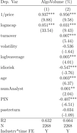
The multivariate regressions in this section confirm that low price results in higher percentage of liquidity provided by algo traders. I control for additional variables to overcome omitted variable bias. The regression specification is

AlgoV olumei,t =uj,t+β∗1/pricei,t+ Γ∗Xi,t (2.1)

uj,t is the industry−by−time fixed effect. The key variable of interest, 1/pricei,t, is the

daily inverse of the stock price. Xi,t are the control variables presented in Table 2.1.

Table 2.1 confirms that AlgoVolume is high for low-price securities, consistent with hy-pothesis I. The table also shows that stocks with larger market cap, more retail trading, and older age have higher percentage of liquidity provided by algo traders. The insignifi-cant coefficients before other variables do not necessarily imply that these variables have no impact on absolute magnitude of the liquidity provision of algo traders. For example, the insignificant coefficient before volatility should be interpreted as that volatility has similar impact on the liquidity provision of algo traders and non-algo traders, and has no statisti-cally significant impact on the ratio of their liquidity provision. The main takeaway from Table 2.1 is that algo traders concentrate their activity on stocks with a low-price securities.

2.4.2

Difference in Difference Analysis

This section examines the causal impact of security price on algorithmic liquidity provision (hypothesis I). Section 2.4.2.1 illustrates how the proportion of the liquidity provided by algo traders is measured. Section 2.4.2.2 presents the difference-in-differences test using the splits/reverse splits of leveraged ETFs as exogenous shocks to price to study the impact of price on algorithmic liquidity provision.

2.4.2.1 Measure of Algo Trader Activity

I use NASDAQ ITCH data to construct a proxy for algorithmic liquidity provision activities. The proxy is called strategic run by Hasbrouck and Saar (12) . A strategic run is a series of submissions, cancellations, and executions that are likely to form an algorithmic strategy. RunsInProcess is the sum of the time length of all strategic runs with 10 or more messages divided by the total trading time of that day (12). Hasbrouck and Saar (12) finds that RunsInProcess has very high correlation with the absolute level of algorithmic market making activities.

Dep. Var AlgoVolume (%) (1) (2) 1/price 0.937*** 0.956*** (9.88) (9.58) logmcap 0.051*** 0.031*** (33.54) (9.43) turnover 0.007*** (5.44) volatility -0.536 (-1.64) logbvaverage 0.005*** (4.01) idiorisk -0.547*** (-3.76) age 0.003*** (6.37) numAnalyst 0.001** (2.04) PIN -0.407*** (-6.51) pastreturn -0.034 (-1.09) R2 0.632 0.664 N 2268 2268 Industry*time FE Y Y

Table 2.1: Price and Algorithmic Liquidity Provision

2.4.2.2 Difference-in-Differences Test using Leveraged ETF Splits/Reverse Splits

This section establishes the causal effect between price, and the percentage of algorithmic liquidity provision using a difference-in-differences test. I use ETF split/reverse split as an exogenous shock to algorithmic liquidity provision. Treatment group would be split/reverse split ETFs. Their pairs that track the same index but do not split / reverse split provide an ideal control. Among ETFs, splits/reverse splits are more frequent for leveraged ETFs. The regression specification for the difference-in-differences test is:

whereyi,t,j is algorithmic liquidity provision activity for ETF j in index i at time t. ui,t, the

index-by-time fixed effects, controls for time-varying algorithmic liquidity provision activity.

γij is the ETF fixed effect that absorbs the time-invariant differences between two leveraged

ETFs that track the same index. The key variable in this regression isDtrti,t,j, the treatment

dummy, which equals 0 for the control group. For the treatment group, the treatment dummy equals 0 before splits/reverse splits and 1 after splits/reverse splits. Coefficient ρ captures the treatment effect.

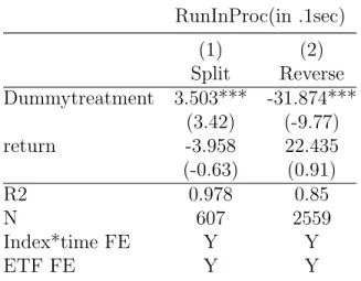
RunInProc(in .1sec) (1) (2) Split Reverse Dummytreatment 3.503*** -31.874*** (3.42) (-9.77) return -3.958 22.435 (-0.63) (0.91) R2 0.978 0.85 N 607 2559 Index*time FE Y Y ETF FE Y Y

Table 2.2: Diff-In-Diff Analysis

Table 2.2 shows an increase in algorithmic liquidity provision activities in the treatment group after splits relative to the control group. Since the analysis has controlled for the index-by-time fixed effect, an increase in algorithmic liquidity provision activities cannot be attributed to the change in the underlying fundamental of the leveraged ETF. Specifically, the increased algorithmic liquidity provision activities cannot be ascribed to information events, because the treatment and the control groups have the same underlying information. The ETF fixed effects and the return variable further control other possible differences between ETFs in the same pair. I argue that the increase in algorithmic liquidity provision activities is driven by price. Splits lead to coarser price grids, which can force traders who quoted different prices before splits to quote the same price after splits, thus causing an increase in the length of the queue at the new but more constrained best price. Column 2 reports a reduction in algorithmic liquidity provision activities following the reverse splits.

In summary, I find that splits increase algorithmic trading activity whereas reverse splits reduce algorithmic liquidity provision activities.

2.5

Price and Algorithmic Trading Revenue

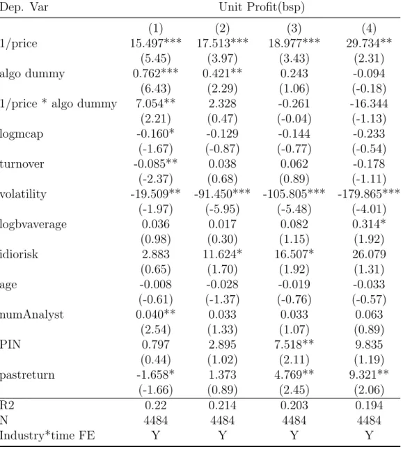
In this section I demonstrate that the revenue is also higher for stocks with lower price. In addition, I find that algo traders do not outperform non-algo traders when they trade on the same stock, which is in disagreement with (9). One plausible explanation is that the superior performance of algo traders comes from their overweight in stocks with high revenue securities. I test hypothesis II using the following specification.

U nitRevenuei,t,n =β1∗AlgoDummyi,t,n+β2∗1/pricei,t +uj,t+ Γ∗Xi,t+i,t,n (2.3)

1. Total Revenue. My revenue measure comes from Brogaard, Hendershott, and Riordan(9) , Menkveld (16) , and Baron, Brogaard, and Kirilenko (5). The algorithmic trading revenue for an individual stocki during for day t is defined as

πAlgo,it =

n

X

1

−(Algoit_n) +INV Algoit_N ∗P_closeit (2.4)

The revenue comes from two components. The first term,Pn

1 −(Algo

it

n), captures total

cash flows throughout the day. I separate day t’s transactions into n blocks, within each block I have N transactions. The second term, often referred as positioning rev-enue, cumulates value changes associated with net position. In the analysis, INV Algo accumulated in dayt is cleared at closing midpoint quotePclose.

2. Unit Revenue. Since I am interested in the market marking revenue per dollar volume, I calculate the unit revenue as:

U nitRevenuei,t,n=πAlgo,it/DolAlgo,it (2.5)

trading revenue per dollar volume of non-algo traders is calculated analogously. In specification 2.3, U nitRevenuei,t,n is the unit revenue for each stock i on date t for

trader type n. There are two daily observations for each stock: a unit revenue for algo traders and a unit revenue for non-algo traders. These unit variables depends on a number of controls Xi,t and two key variables of interest: price and AlgoDummy. AlgoDummyi,t,n

equals 1 for the unit revenue of algo traders and 0 otherwise. 1/pricei,t, is the reverse of

price of stock i at day t. uj,t is the industry−by−time fixed effect. Xi,t are control variables

presented in Table 2.3.

Table2.3 shows that the unit revenue is high for low-price securities for all revenue mea-sures. It also shows that algo traders do not have higher performance than non-algo traders do at stock by stock level . One plausible reason would be algo traders’ overweight in stocks with higher unit revenue .

Dep. Var Unit Profit(bsp) (1) (2) (3) (4) 1/price 15.497*** 17.513*** 18.977*** 29.734** (5.45) (3.97) (3.43) (2.31) algo dummy 0.762*** 0.421** 0.243 -0.094 (6.43) (2.29) (1.06) (-0.18)

1/price * algo dummy 7.054** 2.328 -0.261 -16.344

(2.21) (0.47) (-0.04) (-1.13) logmcap -0.160* -0.129 -0.144 -0.233 (-1.67) (-0.87) (-0.77) (-0.54) turnover -0.085** 0.038 0.062 -0.178 (-2.37) (0.68) (0.89) (-1.11) volatility -19.509** -91.450*** -105.805*** -179.865*** (-1.97) (-5.95) (-5.48) (-4.01) logbvaverage 0.036 0.017 0.082 0.314* (0.98) (0.30) (1.15) (1.92) idiorisk 2.883 11.624* 16.507* 26.079 (0.65) (1.70) (1.92) (1.31) age -0.008 -0.028 -0.019 -0.033 (-0.61) (-1.37) (-0.76) (-0.57) numAnalyst 0.040** 0.033 0.033 0.063 (2.54) (1.33) (1.07) (0.89) PIN 0.797 2.895 7.518** 9.835 (0.44) (1.02) (2.11) (1.19) pastreturn -1.658* 1.373 4.769** 9.321** (-1.66) (0.89) (2.45) (2.06) R2 0.22 0.214 0.203 0.194 N 4484 4484 4484 4484 Industry*time FE Y Y Y Y

Chapter 3

Styled Algorithmic Trading under Mean-Variance

Framework

3.1

Introduction

For major institutional clients such as mutual funds, retirement funds, or hedge funds, algorithmic trading for optimal execution helps liquidate or acquire big positions with limited impacts on both the markets and the clients. The execution houses (e.g., broker-dealers and agencies) in return generate commission revenues to cover their costs on IT infrastructures (e.g., servers or data warehouses), as well as on model and analytical development. Therefore, execution motivated algorithmic trading has become a crucial financial service for modern electronic markets. 2

The most striking characteristics of algorithmic trading, as compared with the one-shot trading activities of small individual investors, is its constant flow of trading decisions made throughout the entire execution horizon. The key is to decide how to best “slice” the entire big order into smaller “child” orders to be progressively executed. Ideally such decisions have to resonate with the real-time dynamics of the markets and inventory positions. Dynamic programming (DP) naturally becomes the central approach to optimal algorithmic trading. This could be witnessed from the pioneering works of Bertsimas and Lo (7), and Huberman and Stanzl (13), to more recent ones by Almgren (1), Bouchard, Dang, and Lehalle (8), and Azencott et al. (4). Static algorithms, e.g., those by Almgren and Chriss (2), Huberman and Stanzl (13), Obizhaeva and Wang (17), Avellaneda and Stoikov (3), Kissell and Mala-mut (15), Gatheral (11), or Shen (24), can provide useful pre-trade estimation for clients. They nevertheless do not respond to fresh market information and thus cannot be designated as actual execution strategies.

While it provides a natural paradigm, DP does impose a number of challenges on both modeling and computing. For instance, since theFlash Crashin the US markets on May 6th, 2011, it has been clear that trading risks can be significantly curbed via setting up even simple constraints like price or volume limits. Thus fundamentally algorithmic trading has to be a constrained DP problem, and closed-form solutions generally do not exist. In Section 3.2, I will discuss in more technical details several outstanding challenges in implementing a self-contained DP trading strategy, including, e.g., (a) defining proper DP objectives meaningful to general traders, (b) properly handling key trading constraints, and (c) efficiently dealing with the explosion of dimensions.

There are two main approaches to answering these challenges in practice, and both are in the approximation sense. The first is to periodically call a static strategy, e.g., every 20 minutes or whenever certain events trigger. This is a heuristic way to emulate dynamic trading via static strategies like that of Almgren and Chriss (2). Traditionally many execu-tion houses have adopted this approach as it is much easier to integrate algorithmic trading with efficient static commercial optimizers such as IBM CPLEX or MOSEK. This heuristic approach can take good care of client constraints but generally lacks a coherent theoretical foundation.

The second way turns to the method ofapproximate dynamic programming(ADP). ADP is currently an active and rapidly evolving research area (e.g., (6, 22)). ADP aims at breaking the curse of dimensionality via properly designed approximation schemes. The approxima-tions may be made for the objectives, state spaces, control acapproxima-tions, state transiapproxima-tions, the policies, or the Bellman equations. Despite such a vast degree of freedom, there exist no ADP design methods that work universally well for arbitrarily given DP problems. The design of an effective ADP scheme often relies on the particular characteristics of the tasks at hand as well as the insights of users (e.g., (26)).

The current work belongs to ADP in the above general sense. I define a style to be a particular choice of the following two components: (1) state variables, and (2) policies built upon these variables. Section 3.3 shall give a more technical account. Traditionally DP trading can only work with additive objectives. A style defined this ways allows a much broader class of trading objectives, including, e.g., the mean-variance utilities of Almgren

and Chriss (2).

The remaining sections demonstrate styled trading via the detailed construction of a par-ticular style using themean-varianceobjective and the two state variables of moneyness and volume participation. For convenience, this particular style is called the MV-MVP strategy. In Section 3.4 I define the two dimensionless state variables - moneyness and forward PoV, and also derive their state transition equations. In Section 3.5 I introduce the mean-variance objective for theaugmentedimplementation shortfall (IS) (19), and define a particular para-metric form of trading policies. The popular VWAP strategy can be considered as a special scenario of MV-MVP when all the four parameters are set to zero. Model calibration is discussed in Section 3.6, in which a generic instance of the MV-MVP style is also worked out.

Below are some important settings or assumptions for the current work.

1. The trading horizon (0, T] is assumed to be an intraday time window, e.g., from 11:15 am to 1:30 pm, within the continuous session. The starting time is always denoted by t = 0. The current work does not cover any auction sessions such as the opens or closes.

2. As in most aforementioned works in the literature, I am primarily concerned with optimal decisions on setting the trade sizes for arrival bins. Let ∆tdenote an internally chosen child window size, e.g., 5 minutes. The trading horizon (0, T] is then “sliced” into N child bins:

(t0, t1,· · · , tN) = (0,∆t,2∆t,· · · , N∆t =T).

At each time tn, the decision is to be made for the number of shares qn to trade over

the arrival bin (tn, tn+1].

3. The current work does not address how to actually execute qnshares within an arrival

bin (tn, tn+1]. This is called the process of Child Order Placement (COP). A COP

strategy often involves the following key components: (a) further slicing each child order into grandchild orders, (b) timing and anti-gaming of placing each grandchild

order, (c) selecting market or limit order types for each grandchild order, and (d) for limit orders determining book sitting levels, waiting times, and cancel-and-replace policies. In particular, one observes that the bin size ∆t should be big enough in order to accommodate any COP limit-order strategies. Otherwise, time may be too short for the limit orders to be traded through.

3.2

Challenges in Dynamic Trading

I first discuss some major challenges that a traditional DP strategy has to face, in order to motivate styled DP trading.

J0(q0,· · ·, qN−1;|ωx0) =

N−1

X

n=0

βngn(xn, qn) +βNgN(xN), (3.1)

where ω denotes a market path, and β ≥0 a potential discount factor. For a single-factor market, one hasω = (ω0,· · · , ωN−1) withωn denoting the scalar random market movement

over (tn, tn+1]. The stagewise cost gn(·,·) and terminal cost gN(·) may be stage dependent,

as indicated by the subscripts. Let Dn(xn) denote the permissible action space for trading

bin n, so that one demands qn ∈ Dn(xn). Dynamical trading is to seek a series of optimal

policies ϕ∗₀(·), ϕ∗₁(·),· · · , ϕ∗_N−1(·), such that (ϕ∗₀,· · · , ϕ∗_N−1) = arg min (ϕ0,···,ϕN−1) Eω[J0(qn=ϕn(xn),0≤n < N;ω |x0)]. (3.2)

At the beginning time tn of (tn, tn+1], define the spot cost

Jn(qn,· · · , qN−1,ω|xn) = N−1

X

k=n

and thespot value function:

vn(xn) = min

(ϕn,···,ϕN−1)

Eω[Jn(qk =ϕk(xk), n≤k < N;ω |xn)]. (3.3)

Then one has the backward recursive Bellman equation: for n=N −1,· · · ,0,

vn(xn) = min qn

{gn(xn, qn) +βEωn[vn+1(Fn(xn, qn, ωn))]}. (3.4)

Here xn+1 =Fn(xn, qn, ωn) is the state transition equation with stage specific market noise

ωn. The main challenges of dynamic algorithmic trading are summarized as follows.

1. Pros and Cons of Additive Costs. Additivity has induced the whole Bellman machinery (i.e., Eqn. (3.4)), but also severely restricted the available class of cost functions. It forces one to either work with the risk-neutral setting or adopt additive risk measures such as thetotal quadratic variance. Both do not explain well to traders who typically request the lowest average implementation shortfalls (IS) given a toler-able risk level. For them, the mean-variance objectives of Almgren and Chriss (2) are more pertinent even though they are non-additive.

2. Completion. A typical trader prefers an algorithm to complete the entire order within a specified trading horizon, say, from 10:00 am to 11:30 am. Most existing works achieve it by setting qN−1 of the last bin (tN−1, tN = T] to be the entire remaining

order (7).

In reality, this may well deplete the entire market over the last bin if the outstanding order significantly dwarfs the market. One simple mechanism in favor of completion is to enforce a minimum participation rule:

qn =ϕn(xn)≥minPoV·Vn (3.5)

3. Explosion of Dimensions. Except for simple and often constraint-free models, e.g., LQR (6), there are typically no closed forms for either the value functionsvn(·)’s or the

optimal policies ϕn(·)’s. Let An(xn) = An ⊆ Rd denote the state space for xn ∈ Rd.

Each optimal policy ϕ∗_n is a mapping:

ϕ∗_n :An(xn)→ Dn(xn), xn →qn∗ =ϕ

∗

n(xn).

Even in the discretized setting, the search space for any single policy ϕ∗_n would have size LM_{, assuming the state space A}

n is discretized to M states, and the action space

Dn toL actions. The search space is usually humongous.

4. Constraints Handling. Besides the completion constraint, typical traders also im-pose the following two constraints:

(a) Monotonicity. That is, for a buy order, one demands: qn ≥ 0 for any n.

Similarly, for a sell order, one requires: qn≤0 for each n.

(b) Volume Participation Limit. Most traders prefer to cap the maximum rate of PoV, such that:

qn ≤maxPoV·Vn, 0≤n < N. (3.6)

This is typically used as the ultimate gate keeper for avoiding market crash, and is especially important for illiquid securities.

Such constraints have not been rigorously enforced in most traditional DP models due to the universal difficulty in accommodating constraints in DP.

3.3

Dynamic Algorithm Trading with Constraints

As the terminology “style” has not yet been commonly circulated in the industry, I first give a more detailed account about styles and style designing.

I define a “style” to be a user’s particular choice of the two key factors:

1. State variables xn = (xn,1,· · · , xn,d) for each bin (tn, tn+1], based on which trading

2. A particular parametric form of trading policies:

qn=ϕn(xn |Θ), n= 1,· · ·, N −1, (3.7)

based on the state variablesxn, and a finite set of parameters Θ. The set of parameters

can be further split to two sets: Θ = Θi ∪Θe. Θe denotes the set of trading control

parameters exposed externally to traders. For example, most clients prefer to cap the volume participation level, e.g. maxPoV = 25%. Θi denotes the subset of remaining

parameters that add further trading control but are internallyoptimized.

As an example, in the execution industry one often hears the terms “aggressive in the money (ITM)” or “passive in the money”. Here,

1. Moneyness must be one of the state variables, which I shall elaborate on later. For the moment, let me denote moneyness by δn.

2. Suppose the buying strategy can be expressed by qn = ϕn(δn,· · · | Θ), and suppose

that for a buy order, ITM is defined as δn < 0. Then the style of “being aggressive

ITM” means that ϕn is monotonically decreasing onδnso that one trades aggressively

when δn becomes more negative.

Since styled trading works with a particular parametric class of policies, it can only be suboptimal compared with the full engine of DP trading. But the gains are also substantial. 1. Significant complexity reduction. Under styled algorithmic trading, one is only re-quired to calibrate a few or several internal parameters Θi, via a lower dimensional

optimization problem.

2. Flexible handling of constraints. For example, most traders prefer to set the volume limit maxPoV. It suffices to choose a style in the form of: (witha∧b = min(a, b))

qn=ϕ(xn|Θ) =gn(xn|Θ)∧(maxPoV·Vn),

To illustrate the main ideas of styled algorithmic trading, for the rest of the paper, I shall focus on designing one specific style called the MV-MVP model. It is built upon the mean-variance (MV) objective and the state variables of moneyness and volume participation (MVP). To some degree, the MV-MVP style extends the popular VWAP algorithm by facilitating extra dynamic response to moneyness.

For simplicity, hereafter I shall use Θ to denote only the internal model parameters Θi.

External parameters Θe are trading parameters set by traders and need no computation.

Model calibration then means to calibrate Θ. For MV-MVP, Θ only contains four scalar parameters (a, b, c, d).

3.4

States and Dynamics Based on Moneyness and Forward PoV

Let (0, T] denote the trading horizon for buying or selling Q shares in total. Since the current model assumes no biases between buy and sell, I shall fix the running example to be a buy order. Following the Introduction, a DP algorithm decides the number of shares qn

to trade over each arrival bin (tn, tn+1 =tn+ ∆t], with ∆t being 1 minute or 5 minutes, for

instance. It then relies upon a sound Child Order Placement (COP) strategy for actually executingqn shares over the bin. A typical COP strategy involves a complex flow of actions

on further grandchild order slicing, limiting order placement, and aggressive spread crossing, etc, as addressed in the Introduction.

3.4.1

State Variables: Moneyness and Forward PoV

Let pn denote the opening price at tn for each bin (tn, tn+1]. In reality, it could be the mid

price of the National Best Bid and Offer (NBBO) at tn, for example. For n = 0, p0 is the

initial arrival price for the entire execution. At each tn, the state variable “moneyness” is

defined by: δn = pn−p0 p0 = pn p0 −1.0, n= 0,1,· · · , N −1. (3.8)

Similarly, for analytical or computational purposes, I define the posterior moneyness ¯δn by: ¯ δn = ¯ pn−p0 p0 = p¯n p0 −1.0,

where ¯pn denotes the average execution price for all qn shares over (tn, tn+1]:

¯ pn= PKn k=1pn,k·qn,k qn , Kn X k=1 qn,k=qn.

Here, (qn,k | 1 ≤ k ≤ Kn) denotes the individual grandchild orders executed by the COP

manager over (tn, tn+1], and (pn,k |1≤k ≤Kn) their execution prices.

Let Q denote the size of the entire order, and Qexe = q0 +q1 +· · · +qN−1 the total

executed shares over the designated horizon (0, T]. For dynamic trading, generally one could only guarantee that Qexe ≤ Q. The realized implementation shortfall (IS) per dollar

is defined to be: ISexe = PN−1 n=0 p¯nqn−p0·Qexe p0·Qexe = 1 Qexe N−1 X n=0 ¯ δn·qn (3.9)

For example, ISexe = 0.0010 means that to buy every $10,000 amount of the security (as

valued at t=t0 = 0), one actually ends up paying $10,010 on average.

By Eqn. (3.9), IS is determined by all theposterior moneyness ¯δn’s which are unavailable

at each planning time tn. They clearly depend on the observables – the state variables of

moneyness δn’s that actually affect trading decisions.

I now introduce the second state variable – the forward PoV νn. At the starting time tn

of each arrival bin (tn, tn+1], I define the residual Qn via:

Q0 =Q, Qn=Qn−1−qn−1, 1≤n≤N, (3.10)

where qn−1 is the shares acquired over the departing bin (tn−1, tn]. Thus Qn represents

the total shares still needed to be executed at tn. Let Mn denote the (projected) total

market volume over the remainder of the execution horizon (tn, T]. In order to minimize

complexities, in the current work I assume market volumes obey a deterministic volume “profile”. In many execution houses, such profiles are often automatically generated by

overnight or over-weekend processes that utilize the most recent market information. I must point out that for general styled trading, one could also introduce randomness into market volumes and a new state variable associated with it. Such a style can be more realistic but also more complex.

At the starting time tn of an arrival bin (tn, tn+1], the forward PoV is defined to be:

νn=

Qn

Mn

, n = 0,1,· · ·, N −1. (3.11) Similar to moneynessδndefined earlier, the forward PoVνnis alsodimensionless. Moreover,

ν0 =

Q0

M0

= Total Shares to Execute over [0, T] Total Market Shares over [0, T] is precisely the PoV for a VWAP algorithm.

3.4.2

State Transitions and Permanent Market Impacts

LetVn =Mn−Mn+1 denote the market volume over (tn, tn+1]. I define the actual PoV over

the bin by:

un =

qn

Vn

, which is dimensionless. (3.12)

For the MV-MVP style being constructed, I define

State Variables: δn, νn; and Control Variables: un. (3.13)

Notice that all three variables are dimensionless.

Letρn = _MVn_n denote the volume percentage of a “current” bin (tn, tn+1] over the remaining

horizon (tn, T]. The forward PoV has the transition equation:

νn+1 = Qn+1 Mn+1 = Qn−Vn·un Mn−Vn = Qn/Mn−Vn/Mn·un 1−Vn/Mn = νn−ρn·un 1−ρn , (3.14)

which is linear since ρn is known given a volume profile.

by the Brownian motion of dPt/P0. Since dδt = dP_Pt

0, in the discrete setting one could thus

assume that

δn+1 =δn+σn

√

∆tZn+ImpactCostn(un), (3.15)

where σn is the (annualized) spot volatility for (tn, tn+1], and Zn an independently drawn

canonical Gaussian. Notice that for intraday trading, I always assume that market buys and sells are in balance so that no directional drift exists. The impact cost of the trading of qn = un·Vn shares is ImpactCostn(un), which affects the execution prices of all trailing

trades over (tn+1, T]. It is thus called the permanent impact. For illustrative purpose, I

assume:

ImpactCostn(un) =µ·σn

√

∆t·uγ_n, (3.16)

with some bin independent exponent γ ∈ (0,1] and coefficient µ > 0. It has been broadly noted (e.g., (15)) that permanent costs are concave functions which requires γ ≤ 1. Since

δn(moneyness), σn(annualized spot volatility), and un(realized PoV) are all dimensionless,

so must be the permanent impact coefficient µ. It is also possible to incorporate the so-called transient impact if necessary, though I will not consider it for the MV-MVP style. Transient impact represents the resilient effects of all the preceding trades un−1, un−2,· · ·

by time tn, and is often expressed as a moving average (see e.g., Obizhara-Wang (17) and

Shen (24)). To summarize, I have established the following state transition equations: for bin n = 0,· · · , N −1: νn+1 = νn−ρn·un 1−ρn , ρn= νn Mn = 1− Mn+1 Mn (3.17) δn+1 =δn+σn √ ∆t·Zn+µσn √ ∆t·uγ_n. (3.18)

The initial state is:

ν0 =

Q M0

, the PoV for VWAP, and δ0 =

p0−p0

p0

3.5

The MV-MVP Style

3.5.1

The Objective, Instantaneous Impact, and Augmented IS Cost

LetQN be the residual shares by the end of an execution horizon tN =T. Generally due to

the cap on volume participation imposed by traders,QN could be non-zero. The number of

executed shares is thus

Qexe=Q−QN =q0+q1+· · ·+qN−1. (3.20)

By the dimensionless Eqn. (3.9), the total dollar amount of the IS becomes

IS_exe$ =p0·Qexe·ISexe =p0·

N−1

X

n=0

¯

δn·qn. (3.21)

The expected difference between the posterior moneyness ¯δn and the moneyness state δn at

tn is modeled by the instantaneous impact. Due to the short span of ∆t, I adopt a linear

model (24): ¯ δn−δn=η·σn √ ∆t·un+ηBB·σn √ ∆t·Zn. (3.22)

The details are as follows.

1. η represents the instantaneous effect, and is in general inversely proportional to either the liquidity level under macro measures of an security (e.g., average daily volume or spread) or the thickness of the limit order book under market microstructures.

2. The canonical Gaussian Zn is the same as in Eqn. (3.15), and theηBB-term represents

the average random cost of all qn shares traded over (tn, tn+1]. Thus ηBB should be

closely correlated to the in-house COP strategies. It can be shown under the theory of Brownian Bridges (14) that if the COP strategies uniformly place individual orders, one hasηBB ≈0.5.

Due to linearity, η and ηBB can be calibrated via linear regression using in-house trading

data. To impose the completion condition softly, I define the residual cost:

IS_res$ = Γ·σp0·QN, (3.23)

where σ denotes the annualized daily volatility, and Γ > 0 is a residual-averse weight to penalize residuals. For instance, one could set Γ = Γ0 ·

q

1

BDAY S, where BDAY S denotes

the number of trading days per year and Γ0 an orderO(1) constant. This way the residual

cost IS$

res is roughly proportional to the overnight holding risk before one could trade the

rest on the next business day.

Introduce the execution profile q= (q0,· · · , qN−1). Combining (3.21) and (3.23), I define

the total augmented IS cost ISΓ=ISΓ(q|Q) per dollar to be:

ISΓ= 1 Q N−1 X n=0 ¯ δn·qn+ Γ·σ QN Q = IS$ exe+ISres$ Q·p0 (3.24)

withQN =Q−q0−q1− · · · −qN−1. It also depends on the market pathω = (Z0,· · · , ZN−1),

as in Eqn. (3.15) and (3.22). Thus one writes ISΓ = ISΓ(q,ω | Q). The objective is to

minimize risk adjusted IS in the mean-variance framework of Almgren and Chriss (2, 24): min

q Eω[ISΓ(q,ω |Q)] +λ·VARω[ISΓ(q,ω|Q)] (3.25) for some given level of risk aversionλ >0. As discussed earlier, traditional dynamic trading can hardly handle such non-additive objectives.

3.5.2

Design of The MV-MVP Style

As in Section 3.4, I shall work with the dimensionless PoV variables un = q_vn_n. Define the

execution PoV profile u= (u0,· · · , uN−1). Then the objective expression (3.25) can also be

written as

min

The particular model being designed is called the MV-MVP style in order to highlight that (a) it is mean-variance based, and (b) the state variables are given by moneyness and volume participation (via forward PoV). The MV-MVP allows two important features.

1. To set a maximum volume participation limit maxPoV ∈(0,100%). Most clients prefer a PoV cap like maxPoV = 10%,15%, or 25%.

2. To enforce a minimum participation rate minPoV. In DP trading, this is to ensure that at least a minimum amount of shares can be executed over a trading horizon, regardless of the actual market conditions.

Consequently I seek a policy in the form of:

un= minPoV∨hn∧maxPoV = min(max(minPoV, hn),maxPoV), (3.27)

where hn is the “free” PoV in the linear form of:

hn =ν0+αn·δn+βn·(νn−ν0), n = 0,1,· · · , N−1. (3.28)

(Be reminded that the running example is for a buy order with un ≥ 0.) Notice that

ν0 = _MQ0₀ = _MQ₀ is exactly the PoV for the VWAP algorithm. Here the two coefficient series

(αn)and (βn) provide further freedom for style design. To proceed, I always assume this

compatibility condition to hold:

minPoV≤ν0 ≤maxPoV. (3.29)

While maxPoV is typically exposed to clients, minPoV could be internally designed. I make the following comments regarding the roles of (αn) and (βn):

1. The free PoV hn in Eqn. (3.28) is like a factor model commonly used in risk

analyt-ics (20), where δn and νn are the two observable factors.

2. The coefficients (αn) effectively express the popular industrial styles of being

a buy order, ITM means δn <0. Then a positive αn would reduce the PoV hn while

being ITM, and thus achieve being “passive ITM”. Similarly, a negative αn amounts

to becoming aggressive ITM.

3. When setting αn ≡ 0.0 and βn ≡ 1.0, n = 0,· · · , N −1, one has hn ≡ νn. In this

scenario one can further show recursively that un ≡ hn ≡ νn ≡ ν0. That is, the

MV-MVP style becomes the canonical VWAP algorithm.

4. Linear policies like Eqn. (3.28) are actual closed-form solutions in the classical constraint-free LQR models (Linear Quadrature Regulators), in which linear state tran-sitions are coupled with stagewise quadratic costs (6).

The computational burden for the policies in Eqn. (3.27) and (3.28) under the mean-variance objective (3.25) is still enormous, as one has to optimize the coefficient series in a high-dimensional space:

(α0, β0;α1, β1;· · · ;αN−1, βN−1)∈R2N.

More importantly, Bellman-type backward procedures do not apply as the mean-variance objective is not additive.

As a result, I complete the design of the MV-MVP style by further choosing an explicit parametric form for the decision coefficients: for n = 0,· · · , N −1,

αn=a· 1− n N −1 1+b , βn = 1 +c· 1− n N −1 1−d , (3.30)

where one only requires b >−1.0 and d <1.0, so that as n approaches the last trading bin

N −1, one has:

αn →0.0, βn →1.0. (3.31)

When a=c= 0.0, one recovers the VWAP algorithm.

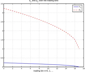
In general, the MV-MVP style allows more active response to moneyness in the beginning of trading. Near the end of an execution horizon, however, it starts to prioritize in the completion requirement by converging to the forward PoV, i.e.,hn →νn.

3.6

Calibration of Styled Trading Models

To summarize, the MV-MVP style eventually becomes an optimization problem with only four unknown parameters (a, b, c, d):

min

(a,b,c,d)F(a, b, c, d) = E[ISΓ(u,ω |Q)] +λ·VAR[ISΓ(u,ω|Q)]. (3.32)

The policy style is defined via the specific parametric form:

             un = minPoV∨hn∧maxPoV, hn =ν0+αn·δn+βn·(νn−ν0), αn=a(1− _Nn₋₁)1+b, βn = 1 +c(1−_Nn₋₁)1−d. (3.33)

Also recall that the state transition equations are:

     δn+1 =δn+µ·σn √ ∆t·uγ n+σn √ ∆tZn, νn+1 = νn₁−₋ρ_ρn_nun, ρn= _Mνn_n = 1− M_Mn+1_n . (3.34)

The initial state is given by δ0 = 0.0 and ν0 = _MQ

0, and the latter is precisely the PoV for

the VWAP algorithm.

Finally, as in the preceding section, along any pathω = (Z0,· · · , ZN−1),

     ISΓ(u,ω |Q) = _Q1 PN −1 n=0 δ¯n·qn+ Γ·σ· QN Q , qn=un·Vn, ¯ δn=δn+η·σn √ ∆t·un+ηBB·σn √ ∆t·Zn. (3.35)

I must remind readers since the model is buy-sell symmetric , I have been consistently working with a buy order for which Q > 0, un, hn > 0. The setting for a sell order is very

similar when working with the absolute or unsigned PoV un and absolute order size Q,

except for that (i) the plus signs in (3.34) for the permanent impact term and that in (3.35) for the instantaneous impact term should both be flipped, and (ii) ¯δn in the first term of

new variable for order type:

side= +1, for a buy, and−1, for a sell,

and place it as a multiplier for the aforementioned three terms.

Let Θ = (a, b, c, d). Then ISΓ(u,ω | Q) can be expressed as ISΓ(Θ,ω | Q), and the

objective (3.32) becomes: min

Θ F(Θ) =E[ISΓ(Θ,ω|Q)] +λ·VAR[ISΓ(Θ,ω|Q)]. (3.36)

Eventually a styled dynamic trading model becomes a parametric model. Due to the nonlinearities associated with the flooring or capping operators, the power exponents in Eqn. (3.33), as well as the nonlinearities in the state equations (3.34), the objective function

F(Θ) = F(a, b, c, d) is generally nonlinear and non-convex. Thus only local optima are sought after via suitably designed iterative schemes. There exists a wealth of literature on optimizing objectives of stochastic nature, and below I briefly describe two major numerical schemes that I have experimented with: stochastic gradient descent and binomial-tree based gradient descent.

For any given set of styled parameters Θ, the objective involves two ensemble statistics - the mean and the variance. Thus one could employ the method of stochastic gradient descent (SGD) by building gradient descending schemes upon Monte-Carlo valuation (23). My extensive experiments have shown that the local optima captured this way are sensitive to initial guesses, and that the convergence usually takes long. Conventional variance re-duction techniques such as the antithetic method do notwork well since the objective isnot monotonic against random market moves.

Alternatively, the binomial-tree based gradient descent (BT-GD) is more stable and works particularly well for horizons with a moderate number of bins, e.g., 90 minutes in the form of 18 bins of 5-minute child windows. In this implementation, the Gaussian market path in Eqn. (3.35)

is approximately implemented by the binomial path:

ω = (U0,· · · , UN−1), Uk ∼B({1,−1},0.5), k= 0,· · ·, N −1,

where Uk’s are i.i.d.’s of a symmetric Bernoulli type B({1,−1},0.5):

Prob(Uk = 1) = Prob(Uk =−1) = 0.5.

All binomial paths are equally likely under this setting, and the objective function for any given parameter set Θ can be evaluated exactly.

At each iteration step with the “current” estimator Θ0 _{= (θ}0

1, θ02, θ30, θ04) (corresponding to

(a, b, c, d)), the gradient is estimated via synchronized finite differencing as follows. Define the basis directions:

e1 = (1,0,0,0), · · ·, e4 = (0,0,0,1).

For a set of small parameters (ε1,· · · , ε4) fixed throughout the iteration, the gradient

com-ponents are estimated via the central difference scheme:

∂F(Θ0₎

∂θi

=F(Θ0+εiei)−F(Θ0−εiei)

/2i, i= 1,2,3,4.

The evaluation of the eight objective valuesF(Θ0_±ε

iei), i= 1,2,3,4 is synchronized over all

market paths. That is, for each evolving market pathω, the eightISΓ’s associated with the

eight sets of trading parameters are simultaneously computed and recorded. This improves computational efficiency.

As mentioned earlier, the VWAP strategy is a special instance of the MV-MVP style when:

a =b = 0 (i.e.,αn ≡0), and c=d= 0 (i.e., βn≡1).

This provides a natural set of initial guess for any iterative scheme.

Below I demonstrate the behavior of the proposed MV-MVP model via one generic numer-ical instance. I explain it via a pseudo object-oriented fashion, in order to facilitate popular production languages such as C++, Java, or Python.

1. I assume that the market object has the following data fields:

market.dayInMinutes=390, market.yearInBusinessDays=252.

This is to simulate aregularUS equities market which trades from 9:30 am to 4:00 pm (except for special half-days), and has about 252 trading days per year.

2. For illustrative purposes, I assumeflatprofiles of intraday volatilities and volumes, and the particular security object contains this information:

security.ID="ABC", security.vol=25.0%, security.ADV=4,000,000.

Here theaverage daily volume(ADV) of 4 million shares represents roughly the average ADV of S&P 500 stocks, which are large-cap and popularly traded. As common in finance, the volatility is annualized. An annual volatility of 25.0% is roughly the average level of the S&P 500 universe.

3. The trading object trade summarizes both the external trading request from a client and internal trading conventions. For the particular instance, it is assumed that:

trade.startIdx=30, trade.endIdx=120, trade.binWindow=5,

trade.maxPoV=25%, trade.minPoV=2.5%, trade.tradeSize=92300, trade.side="BUY".

That is, the trade request is to buy 92300 shares from 10:00am to 11:30am, with PoV capped at 25.0% and floored at 2.5%. The algorithm also internally sets bin size to 5 minutes. The order size corresponds to the 10% PoV for a VWAP strategy over the same horizon.

4. The model object model is assumed to have the following data fields. In reality, these impact model parameters have to be calibrated from the real trading database. In reality, risk aversion λ is internally mapped to the user-friendly external GUI fields like “Urgency Level.”

I have set ηBB = 0.5 as explained earlier.

Given the above instance of themarket, security, trade,andmodel, my binomial-tree based calibrator converges at the following set of policy parameters:

a = 0.23, b =−0.48; c= 2.24, d= 0.48.

The resulting policy coefficients ofαn’s andβn’s are plotted in Figure 3.1 via the Eqn. (3.30).

0 2 4 6 8 10 12 14 16 18 0 0.5 1 1.5 2 2.5 3 3.5 trading bin n=0, 1, ...

α_n and β_n over the trading bins

α_n βn

Figure 3.1: αn and βn Over The Trading Bin

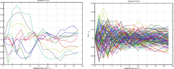
To better visualize the calibrated MV-MVP style, in Figure 3.2 I have plotted the sim-ulated trading paths given 10 or 100 independently simsim-ulated market paths, according to the dynamic policies in Eqn. (3.27) and (3.28). Left: 10 trading paths; Right: 100 trading paths. Both are based on independently simulated market paths. As a reference, pay atten-tion that the original total posiatten-tion has been designed so that the VWAP PoV is 10%. The simulated trading paths oscillate around VWAP for different market scenarios as expected. The MV-MVP incorporates a new degree of dynamic response to the moneyness.

0 2 4 6 8 10 12 14 16 18 0.06 0.07 0.08 0.09 0.1 0.11 0.12 0.13 0.14 0.15 0.16 Dynamic PoV’s trading bin n=0, 1, ... PoV: u n 0 2 4 6 8 10 12 14 16 18 0.04 0.06 0.08 0.1 0.12 0.14 0.16 0.18 Dynamic PoV’s trading bin n=0, 1, ... PoV: u n

Appendix A

AlgoV olumei,t =

%of vol with AlgoT rader as market maker f or stock i on date t T otal trading volume f or stock i on date t

References

[1] R. Almgren. Optimal trading with stochastic liquidity and volatility. SIAM J. Financial

Math., 3:163–181, 2012.

[2] R. Almgren and N. Chriss. Optimal execution of portfolio transactions. J. Risk, 3:5–39, 2000.

[3] M. Avellaneda and S. Stoikov. High-frequency trading in a limit order book. Quant. Finance,

8(3):217–224, 2008.

[4] R. Azencott, A. Beri, Y. Gadhyan, N. Joseph, C.-A. Lehalle, and M. Rowley. Realtime market

microstructure analysis: online transaction cost analysis. ArXiv e-prints, arXiv1302.6363,

http://adsabs.harvard.edu/abs/2013arXiv1302.6363A, 2013.

[5] Matthew Baron, Jonathan Brogaard, and Andrei A Kirilenko. Risk and return in high

fre-quency trading. Available at SSRN 2433118, 2014.

[6] D. P. Bertsekas. Dynamic Programming and Optimal Control. Athena Scientific, 2007.

[7] D. Bertsimas and A. W. Lo. Optimal control of execution costs. J. Financial Markets, 1(1):1–

50, 1998.

[8] B. Bouchard, N.-M. Dang, and C.-A. Lehalle. Optimal control of trading algorithms: a general

impulse control approach. SIAM J. Finan. Math., 2(1):404–438, 2011.

[9] Jonathan Brogaard, Terrence Hendershott, and Ryan Riordan. High-frequency trading and

price discovery. Review of Financial Studies, 2014.

[10] Justin Dove. Is High Frequency Trading Causing Higher

Volatil-ity?, 2011. http://www.investmentu.com/article/detail/23278/

high-frequency-trading-causing-volatility#.VT1Z7CFVhHw.

[11] J. Gatheral. No-dynamic-arbitrage and market impact. Quant. Fin., 10(7):749–759, 2010.

[12] Joel Hasbrouck and Gideon Saar. Low-latency trading. Journal of Financial Markets,

16(4):646 – 679, 2013. High-Frequency Trading.

[13] G. Huberman and W. Stanzl. Optimal liquidity trading. Yale School of Management Working

Papers, YSM 165, 2001.

[14] I. Karatzas and S. Shreve. Brownian Motion and Stochastic Calculus. Springer, 1991.

[15] R. Kissell and R. Malamut. Algorithmic decision making framework. J. Trading, 1(1):12–21,

2006.

[16] Albert J. Menkveld. High frequency trading and the new market makers. Journal of Financial

Markets, 16(4):712 – 740, 2013. High-Frequency Trading.

[17] A. Obizhaeva and J. Wang. Optimal trading strategy and supply/demand dynamics. J.

Financial Markets, 16(1):1–32, 2013.

[18] Scott Patterson. High-Speed Stock Traders Turn to Laser Beams, 2014. http://www.wsj.

[19] A. F. Perold. The implementation shortfall: Paper versus reality. J. Portfolio Management, 14:4–9, 1988.

[20] B. Pfaff. Financial Risk Modelling and Portfolio Optimization with R. Wiley, 2013.

[21] Matt Phillips. Nasdaq: Heres Our Timeline of the Flash Crash, 2010. http://blogs.wsj.

com/marketbeat/2010/05/11/nasdaq-heres-our-timeline-of-the-flash-crash/.

[22] W. B. Powell. Approximate Dynamic Programming: Solving the Curses of Dimensionality.

Wiley, 2011.

[23] A. Shapiro and Y. Wardi. Convergence analysis of gradient descent stochastic algorithms. J.

Optim. Theory Appl., 91(2):439–454, 1996.

[24] J. Shen. A pre-trade algorithmic trading model under given volume measures and generic

price dynamics. Applied Math. Res. Express, Oxford Univ. Press, in press, 2014.

[25] Jackie Shen and Yingjie Yu. Styled algorithmic trading and the mv-mvp style. Available at

SSRN 2507002, 2014.

[26] Y. Wang, B. O’Donoghue, and S. Boyd. Approximate dynamic programming via iterated

Bellman inequalities. Int. J. Robust Nonlinear Control, DOI: 10.1002/rnc.3152, 2014.

[27] Chen Yao and Mao Ye. Tick size constraints, market structure, and liquidity. Unpublished