Stochastic systems model assessment of historical cow-calf biological and economic efficiency for different mature cow weight and peak lactation combinations in the Kansas Flint Hills

(1)

Stochastic systems model assessment of historical cow-calf biological and economic efficiency for different mature cow weight and peak lactation combinations in the Kansas

Flint Hills

by

Dustin Grant Aherin

B.S., Kansas State University, 2014 M.S., Kansas State University, 2017

AN ABSTRACT OF A DISSERTATION

submitted in partial fulfillment of the requirements for the degree DOCTOR OF PHILOSOPHY

Department of Diagnostic Medicine/Pathobiology College of Veterinary Medicine

KANSAS STATE UNIVERSITY Manhattan, Kansas

(2)

Abstract

A stochastic, individual based systems simulation model describing U.S. beef cow-calf production was developed. Accounting for genetics, nutrition, reproduction, growth, health, and economics, allows analysis of various scenario outcomes encompassing different genetic, management, and marketing strategies. The model’s stochastic nature enables consideration of biological variation and probabilistic risk, while the systems design accounts for time delays and complex, prolonged feedback structure, all inherent to beef production. Any number of production years and iterations can be simulated. These capabilities make it ideal for decision analysis and assessment of long-run outcomes regarding a multitude of metrics simultaneously.

Parameterizing the model to match Kansas Flint Hills production and economic conditions for the years 1995 through 2018, 32 breeding systems with different genetic combinations for mature cow weight and peak lactation potential were simulated 100 iterations each. Sire mature cow weight genetics ranged from 454 kg to 771 kg in 45 to 46 kg increments. Sire peak lactation genetics were considered at 6.8, 9, 11.3, and 13.6 kg/d for all eight mature cow weights. Retaining replacement females, the breeding herd size goal was 100 animals. Model decision rules aimed to meet individual animal nutrient requirements.

Utilizing model results for the years 2000-2018, three different validation procedures were applied. A six person panel with combined expertise spanning veterinary medicine, animal breeding and genetics, ruminant nutrition, agricultural economics, and beef production modeling reviewed model output in both absolute and comparative scenario terms. Separately, raw model results were assessed against actual historical cow-calf production

(3)

data. Finally, exploratory factor analysis was applied to interpret the underlying factor scores of model output relative to real-world cow-calf production data.

In cow-calf production, biological and economic efficiency are not perfectly synonymous. Research simultaneously assessing both the biological and economic efficiency of different mature cow weight and peak lactation combinations for twenty-first century cow-calf production is scarce to non-existent. Aggregating simulation results for the 2000 through 2018 production years, under the specific parameters previously described, larger, heavier milking cows exceled in kilograms weaned per cow exposed, while kilograms weaned per net energy for maintenance (kg/Mcal*100) favored smaller, heavier milking cows. Assuming no price differentiation between weaned calves from different breeding systems, 454 and 499 kg mature cow weight with 13.6 kg/d peak lactation had the highest median annual enterprise return on investment (fed ration, pasture, replacement, and interest expenses) at 8.9 and 7.4 percent, respectively. Applying the assumptions that herds comprised of 454 and 499 kg mature cow weight with 13.6 kg/d peak lactation do not exist and that all weaned calves from 454 kg mature cow weight breeding systems receive a small frame price discount, the 544 kg mature cow weight-13.6 kg/d peak lactation combination generated the greatest median annual return on investment at 7.0 percent. Several combinations of 499, 544, 590, and 635 kg mature cow weights with 11.3 or 13.6 kg/d peak lactation produced a median annual return on investment between 4.1 percent and 5.4 percent.

(4)

Stochastic systems model assessment of historical cow-calf biological and economic efficiency for different mature cow weight and peak lactation combinations in the Kansas

Flint Hills

by

Dustin Grant Aherin

B.S., Kansas State University, 2014 M.S., Kansas State University, 2017

A DISSERTATION

submitted in partial fulfillment of the requirements for the degree DOCTOR OF PHILOSOPHY

Department of Diagnostic Medicine/Pathobiology College of Veterinary Medicine

KANSAS STATE UNIVERSITY Manhattan, Kansas 2020 Approved by: Co-Major Professor Dr. Robert L. Larson Approved by: Co-Major Professor Dr. Robert L. Weaber

(5)

Copyright

(6)

Abstract

Parameterizing the model to match Kansas Flint Hills production and economic conditions for the years 1995 through 2018, 32 breeding systems with different genetic combinations for mature cow weight and peak lactation potential were simulated 100 iterations each. Sire mature cow weight genetics ranged from 454 kg to 771 kg in 45 to 46 kg increments. Sire peak lactation genetics were considered at 6.8, 9, 11.3, and 13.6 kg/d for all eight mature cow weights. Retaining replacement females, the breeding herd size goal was 100 animals. Model decision rules aimed to meet individual animal nutrient requirements.

Utilizing model results for the years 2000-2018, three different validation procedures were applied. A six person panel with combined expertise spanning veterinary medicine, animal breeding and genetics, ruminant nutrition, agricultural economics, and beef production modeling reviewed model output in both absolute and comparative scenario terms. Separately, raw model results were assessed against actual historical cow-calf production

(7)

data. Finally, exploratory factor analysis was applied to interpret the underlying factor scores of model output relative to real-world cow-calf production data.

In cow-calf production, biological and economic efficiency are not perfectly synonymous. Research simultaneously assessing both the biological and economic efficiency of different mature cow weight and peak lactation combinations for twenty-first century cow-calf production is scarce to non-existent. Aggregating simulation results for the 2000 through 2018 production years, under the specific parameters previously described, larger, heavier milking cows exceled in kilograms weaned per cow exposed, while kilograms weaned per net energy for maintenance (kg/Mcal*100) favored smaller, heavier milking cows. Assuming no price differentiation between weaned calves from different breeding systems, 454 and 499 kg mature cow weight with 13.6 kg/d peak lactation had the highest median annual enterprise return on investment (fed ration, pasture, replacement, and interest expenses) at 8.9 and 7.4 percent, respectively. Applying the assumptions that herds comprised of 454 and 499 kg mature cow weight with 13.6 kg/d peak lactation do not exist and that all weaned calves from 454 kg mature cow weight breeding systems receive a small frame price discount, the 544 kg mature cow weight-13.6 kg/d peak lactation combination generated the greatest median annual return on investment at 7.0 percent. Several combinations of 499, 544, 590, and 635 kg mature cow weights with 11.3 or 13.6 kg/d peak lactation produced a median annual return on investment between 4.1 percent and 5.4 percent.

(8)

viii

Chapter 3 - Stochastic systems model assessment of cow-calf biological and economic efficiency for different mature weight and peak lactation combinations in the Kansas Flint Hills ... 88 Abstract ... 88 Introduction ... 90 Biological Efficiency ... 90 Economic Efficiency ... 92 Systems Modeling ... 95 Objectives ... 95

Materials and Methods ... 96

Model Simulation... 96

Economics ... 98

Return over Fed Ration, Pasture, Replacement, and Interest Expense ... 99

Financial Equations ... 101

Efficiency Metrics ... 103

Results and Discussion ... 106

Biological Efficiency ... 106

(10)

x

General ... 123

Appendix 3.1: Model Parameters ... 137

Appendix 3.2: Model Output ... 162

Percent Pregnant at Diagnosis ... 162

Weaning Age ... 163

Forage Production ... 164

Kilograms Weaned per Cow Exposed ... 165

Weaning Weight ... 167

Kilograms Weaned per Hundred NEm Intake ... 171

Annual Return per Breeding Female ... 173

Annual Return per Grazing Acre ... 175

Return on Investment ... 178

Revenue per Cow ... 184

(11)

xi

List of Figures

Chapter 2

Figure 2.1. Boxplots representing the median, 25th percentile, and 75th percentile for individual calf birth weight from IND CHAPS and IND MOD. ... 47 Figure 2.2. Boxplots representing the median, 25th_{percentile, and 75}th_{percentile for}

individual calf 205d adjusted weaning weight from IND CHAPS and IND MOD. ... 47 Figure 2.3. Boxplots representing the median, 25th percentile, and 75th percentile for

individual calf weaning age from IND CHAPS and IND MOD. ... 48 Figure 2.4. Boxplots representing the median, 25th_{percentile, and 75}th_{percentile for}

individual cow age from IND CHAPS and IND MOD. ... 48 Figure 2.5. Boxplots representing the median, 25th percentile, and 75th percentile for

yearly mean calf birth weight by cow MW and PL category combination from Herd MOD and HERD CHAPS. MW and PL category could not be identified for HERD CHAPS ... 49 Figure 2.6. Boxplots representing the median, 25th percentile, and 75th percentile for

yearly mean pre-weaning ADG by cow MW and PL category combination from Herd MOD and HERD CHAPS. MW and PL category could not be identified for HERD CHAPS. ... 50 Figure 2.7. Boxplots representing the median, 25th_{percentile, and 75}th_{percentile for}

(12)

xii

MOD and HERD CHAPS. MW and PL category could not be identified for HERD CHAPS. ... 50 Figure 2.8. Boxplots representing the median, 25th percentile, and 75th percentile for

yearly mean cow age by cow MW and PL category combination from Herd MOD and HERD CHAPS. MW and PL category could not be identified for HERD CHAPS. ... 51 Figure 2.9. Boxplots representing the median, 25th percentile, and 75th percentile for

percent pregnant per cow exposed by cow MW and PL category combination from Herd MOD and HERD CHAPS. MW and PL category could not be

identified for HERD CHAPS. ... 51 Figure 2.10. Boxplots representing the median, 25th percentile, and 75th percentile for

percent pregnancy loss per cow exposed by cow MW and PL category

combination from Herd MOD and HERD CHAPS. MW and PL category could not be identified for HERD CHAPS. ... 52 Figure 2.11. Boxplots representing the median, 25th percentile, and 75th percentile for

percent calf mortality per calf born by cow MW and PL category combination from Herd MOD and HERD CHAPS. MW and PL category could not be

identified for HERD CHAPS. ... 52 Figure 2.12. Individual calf factor score plot. birthwt = actual calf birth weight (ABW),

wt205 = calf 205 d adjusted weaning weight (ADJ WW), age = calf weaning age (WAGE), CowAge = cow age (CAGE), and Mature Cow Weight = MW category (MW). Blue lines represent variables’ direction and magnitude of influence based

(13)

xiii

on their factor loadings. Data ellipses represent the two sd factor score coordinate boundary. ... 53 Figure 2.13. Yearly herd data factor score plot Reproduction Factor by Calf Weight

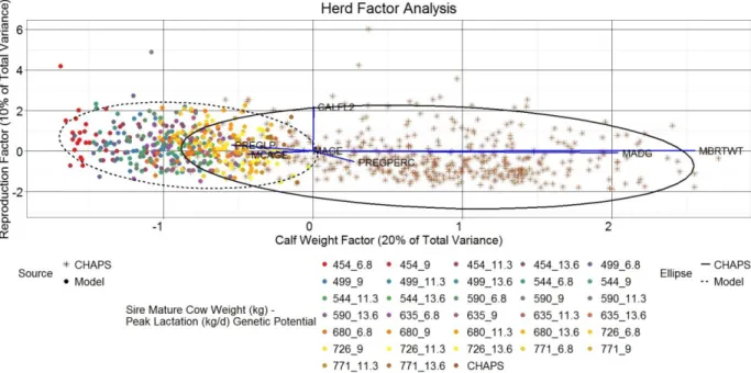
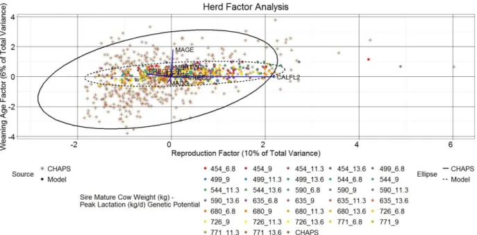
Factor. MBRTWT = mean actual calf birthweight, MAGE = mean calf weaning age, MADG = mean pre-weaning ADG, MCAGE = mean cow age, PREGPERC = percent pregnant per cow exposed, PREGLP = percent pregnancy loss per cow exposed, and CALFL2 = percent calf mortality per calf born. Blue lines represent variables’ direction and magnitude of influence based on their factor loadings. Data ellipses represent the two sd factor score coordinate boundary. ... 54 Figure 2.14. Yearly herd data factor score plot Weaning Age Factor by Calf Weight

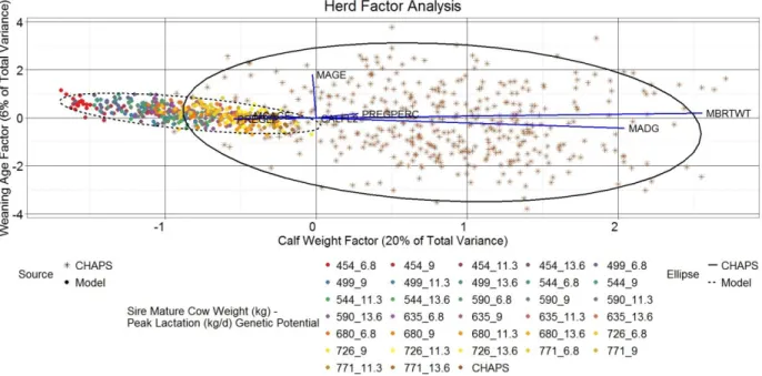
Factor. MBRTWT = mean actual calf birthweight, MAGE = mean calf weaning age, MADG = mean pre-weaning ADG, MCAGE = mean cow age, PREGPERC = percent pregnant per cow exposed, PREGLP = percent pregnancy loss per cow exposed, and CALFL2 = percent calf mortality per calf born. Blue lines represent variables’ direction and magnitude of influence based on their factor loadings. Data ellipses represent the two sd factor score coordinate boundary ... 55

Chapter 3

Figure 3.1 Boxplots representing the median, 25th percentile, and 75th percentile of KPC SPA aggregated across all iterations and production years 2000 through 2018 for each MW and PL category combination. ...107 Figure 3.2. Median KPC SPA across all MW and PL category combinations for all

(14)

xiv

Figure 3.3. Boxplots representing the median, 25th percentile, and 75th percentile of KW NEmH aggregated across all iterations and production years 2000 through 2018 for each MW and PL category combination. ...110 Figure 3.4. Median KW NEmH by MW category across all iterations for each production

year from 2000 through 2018. ...111 Figure 3.5. Median KW NEmH by PL category across all iterations for each production

year from 2000 through 2018. ...112 Figure 3.6. Boxplots representing the median, 25th percentile, and 75th percentile of

annual return over fed ration, pasture, replacement, and interest expense per breeding female aggregated across all iterations and production years 2000

through 2018 for each MW and PL category combination...113 Figure 3.7. Columns represent the top eight (25%) MW and PL category combinations

across all iterations ranked by median return over fed ration, pasture, replacement, and interest expense per breeding female for each production year from 2000 through 2018. ...115 Figure 3.8. Columns represent the median return over fed ration, pasture, replacement,

and interest expense per breeding female by MW category across all iterations for each production year from 2000 through 2018. Dots represent the average base ration price per 10 kg DM and the September price per kg for a 226 kg steer for each production year. Ration and cattle prices are exogenous variables based on historical data. ...115

(15)

xv

Figure 3.9. Columns represent the median return over fed ration, pasture, replacement, and interest expense per breeding female by PL category across all iterations for each production year from 2000 through 2018. Dots represent the average base ration price per 10 kg DM and the September price per kg for a 226 kg steer for each production year. Ration and cattle prices are exogenous variables based on historical data. ...116 Figure 3.10. Boxplots representing the median, 25th percentile, and 75th percentile of

annual return over fed ration, pasture, replacement, and interest expense per grazing acre aggregated across all iterations and production years 2000 through 2018 for each MW and PL category combination. ...117 Figure 3.11. Columns represent the median return over fed ration, pasture, replacement,

and interest expense per grazing acre by MW category across all iterations for each production year from 2000 through 2018. Dots represent the average base ration price per 10 kg DM and the September price per kg for a 226 kg steer for each production year. Ration and cattle prices are exogenous variables based on historical data. ...118 Figure 3.12. Columns represent the median return over fed ration, pasture, replacement,

and interest expense per grazing acre by PL category across all iterations for each production year from 2000 through 2018. Dots represent the average base ration price per 10 kg DM and the September price per kg for a 226 kg steer for each production year. Ration and cattle prices are exogenous variables based on

(16)

xvi

Figure 3.13. Boxplots representing the median, 25th percentile, and 75th percentile of annual ROI (return on fed ration, pasture, replacement, and interest expense) aggregated across all iterations and production years 2000 through 2018 for each MW and PL category combination. ...120 Figure 3.14. Columns represent the median annual ROI (return on fed ration, pasture,

replacement, and interest expense) by MW category across all iterations for each production year from 2000 through 2018. Dots represent the average base ration price per 10 kg DM and the September price per kg for a 226 kg steer for each production year. Ration and cattle prices are exogenous variables based on

historical data. ...121 Figure 3.15. Columns represent the median annual ROI (return on fed ration, pasture,

replacement, and interest expense) by PL category across all iterations for each production year from 2000 through 2018. Dots represent the average base ration price per 10 kg DM and the September price per kg for a 226 kg steer for each production year. Ration and cattle prices are exogenous variables based on

historical data. ...122 Figure 3.16. Columns represent the top eight (25%) MW and PL category combinations

across all iterations ranked by median annual ROI (return on fed ration, pasture, replacement, and interest expense) for each production year from 2000 through 2018...122

(17)

xvii

Chapter 3- Appendix 3.2

Figure 3.A2.1. Boxplots representing the median, 25th_{percentile, and 75}th_{percentile of} PPD aggregated across all iterations and production years 2000 through 2018 for each MW and PL category combination. ... 162 Figure 3.A2.2. Boxplots representing the median, 25th percentile, and 75th percentile of

weaning age aggregated across all iterations and production years 2000 through 2018 for each MW and PL category combination. ... 163 Figure 3.A2.3. Columns represent the median forage yield across all MW and PL

category combinations and iterations for each production year 2000 through 2018. ... 164 Figure 3.A2.4. Median KPC SPA by MW category across all iterations for each

production year from 2000 through 2018. ... 165 Figure 3.A2.5. Median KPC SPA by PL category across all iterations for each production year from 2000 through 2018. ... 166 Figure 3.A2.6. Boxplots representing the median, 25th percentile, and 75th percentile of

actual weaning weight aggregated across all iterations and production years 2000 through 2018 for each MW and PL category combination... 167 Figure 3.A2.7. Median adjusted WW on a steer base, median steer WW genetic potential,

and median actual WW unadjusted for sex across all MW and PL category

(18)

xviii

Figure 3.A2.8. Columns represent the top eight (25%) MW and PL category

combinations across all iterations ranked by median return per grazing acre for each production year from 2000 through 2018. ... 177 Figure 3.A2.9. Boxplots representing the median, 25th_{percentile, and 75}th_{percentile of}

annual revenue per cow aggregated across all iterations and production years 2000 through 2018 for each MW and PL category combination... 184 Figure 3.A2.10. Columns represent the median revenue per breeding female by MW

category across all iterations for each production year from 2000 through 2018. Dots represent the September price per kg for a 226 kg steer for each production year. Cattle prices are exogenous variables based on historical data. ... 185 Figure 3.A2.11. Columns represent the median revenue per breeding female by PL

category across all iterations for each production year from 2000 through 2018. Dots represent the September price per kg for a 226 kg steer for each production year. Cattle prices are exogenous variables based on historical data. ... 186 Figure 3.A2.12. Boxplots representing the median, 25th percentile, and 75th percentile of

annual variable expense per cow aggregated across all iterations and production years 2000 through 2018 for each MW and PL category combination. ... 187 Figure 3.A2.13. Columns represent the median variable expense per breeding female by

MW category across all iterations for each production year from 2000 through 2018. Dots represent the September price per kg for a 226 kg steer for each production year. Cattle prices are exogenous variables based on historical data. ... 188

(19)

xix

Figure 3.A2.14. Columns represent the median variable expense per breeding female by PL category across all iterations for each production year from 2000 through 2018. Dots represent the September price per kg for a 226 kg steer for each production year. Cattle prices are exogenous variables based on historical data. ... 189

(20)

xx

List of Tables

Chapter 2

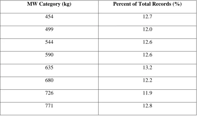
Table 2.1. MLPM decision variable descriptions. ... 37 Table 2.2. MLPM parameter variable descriptions. ... 37 Table 2.3. Expert panel qualifications and experience. ... 41 Table 2.4. Percent of total records in each MW category for IND CHAPS data set

consisting of 5025 unique records from 1642 cows and 6 herds. ... 42 Table 2.5. Percent of total records in each MW category for the model sample data set

consisting of 5025 unique records. ... 43

Chapter 2- Appendix 2.1

Table 2.A1.1. Initialization parameters... 66 Table 2.A1.2. Four-year rolling average Angus genetic trend for birth weight and

weaning weight from 1992 to 2018. ... 67 Table 2.A1.3. Genetic correlations. ... 68 Table 2.A1.4. Manhattan, KS January through August Cumulative Precipitation. ... 69 Table 2.A1.5. Grazing acre allocation for the eight scenario possibilities for mean mature

cow weight. ... 70 Table 2.A1.6. Ration nutrient densities by month. ... 71 Table 2.A1.7. Assorted nutrition parameters. ... 72

(21)

xxi

Table 2.A1.8. Daily maximum DMI as percent of SBW by MW category and animal

production category. ... 73

Table 2.A1.8 (cont.) Daily maximum DMI as percent of SBW by MW category and animal production category. ... 74

Table 2.A1.8 (cont.) Daily maximum DMI as percent of SBW by MW category and animal production category. ... 75

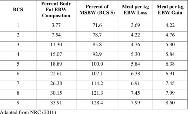
Table 2.A1.9. BCS and corresponding body fat composition, percent of MSBW, and Mcal per kilogram of EBW loss and EBW gain. ... 76

Table 2.A1.10. Maximum base fed ration intake by animal production category... 77

Table 2.A1.11. Reproductive cyclicity. ... 78

Table 2.A1.11 (cont). Reproductive cyclicity. ... 79

Table 2.A1.12. Culling... 82

Table 2.A1.13. Morbidity and mortality. ... 83

Table 2.A1.13 (cont). Morbidity and mortality. ... 84

Table 2.A1.13 (cont). Morbidity and mortality. ... 85

Table 2.A1.14. Calf growth. ... 86

(22)

xxii

Chapter 3

Table 3.1. The top eight (25%) MW and PL category combinations aggregated across all iterations and production years 2000 through 2018 ranked by median annual ROI (return on fed ration, pasture, replacement, and interest expense) assuming all simulated MW and PL combinations exist and no price differentiation between calves from different MW breeding systems. ... 124 Table 3.2. The top eight MW and PL category combinations aggregated across all

iterations and production years 2000 through 2018 ranked by median annual ROI (return on fed ration, pasture, replacement, and interest expense) assuming 454 kg MW-13.6 kg/d PL and 499 kg MW-13.6 kg/d PL cows do not exist, and applying a $0.13/kg discount to the remaining 454 kg MW categories. ... 126

Chapter 3- Appendix 3.1

Table 3.A1.1. Initialization parameters... 137 Table 3.A1.2. Four-year rolling average Angus genetic trend for birth weight and

weaning weight from 1992 to 2018. ... 138 Table 3.A1.3. Genetic correlations. ... 139 Table 3.A1.4. Price multipliers. ... 140 Table 3.A1.5. Manhattan, KS January through August Cumulative Precipitation. ... 141 Table 3.A1.6. Grazing acre allocation for the eight scenario possibilities for sire mature

cow weight genetic potential. ... 142 Table 3.A1.7. Model parameters for grazing expense (USD/per acre). ... 143

(23)

xxiii

Table 3.A1.8. Ration nutrient densities by month. ... 144 Table 3.A1.9. Assorted nutrition parameters. ... 145 Table 3.A1.10. Daily maximum DMI as percent of SBW by MW category and animal

production category. ... 146 Table 3.A1.10 (cont.). Daily maximum DMI as percent of SBW by MW category and

animal production category. ... 147 Table 3.A1.10 (cont.). Daily maximum DMI as percent of SBW by MW category and

animal production category. ... 148 Table 3.A1.11. BCS and corresponding body fat composition, percent of MSBW, and

Mcal per kilogram of EBW loss and EBW gain. ... 149 Table 3.A1.12. Maximum base fed ration intake by animal production category... 150 Table 3.A1.13. Reproductive cyclicity. ... 151 Table 3.A1.13 (cont.). Reproductive cyclicity. ... 152 Table 3.A1.13 (cont.). Reproductive cyclicity. ... 153 Table 3.A1.13 (cont.). Reproductive cyclicity. ... 154 Table 3.A1.14. Culling... 155 Table 3.A1.15. Morbidity and mortality. ... 156 Table 3.A1.15 (cont.). Morbidity and mortality. ... 157 Table 3.A1.15 (cont.). Morbidity and mortality. ... 158 Table 3.A1.16. Calf growth. ... 159

(24)

xxiv

Table 3.A1.16 (cont.). Calf growth. ... 160 Table 3.A1.17. Effective annual interest rates ... 161

Chapter 3- Appendix 3.2

Table 3.A2.1. Median actual calf WW aggregated across all iterations and production years 2000 through 2018 by MW category... 168 Table 3.A2.2. Median actual calf WW aggregated across all iterations and production

years 2000 through 2018 by PL category. ... 169 Table 3.A2.3. Median KW NEmH aggregated across all iterations and production years

2000 through 2018 by MW category. ... 171 Table 3.A2.4. Median NEmH aggregated across all iterations and production years 2000

through 2018 by PL category. ... 172 Table 3.A2.5. Median and interquartile range for annual return per breeding female

aggregated across all iterations and production years 2000 through 2018 by MW category. ... 173 Table 3.A2.6. Median and interquartile range annual return per breeding female

aggregated across all iterations and production years 2000 through 2018 by PL category. ... 174 Table 3.A2.7. Median and interquartile range for annual return per grazing acre

aggregated across all iterations and production years 2000 through 2018 by MW category. ... 175

(25)

xxv

Table 3.A2.8. Median and interquartile range for annual return per grazing acre aggregated across all iterations and production years 2000 through 2018 by PL category. ... 176 Table 3.A2.9. Median and interquartile range for annual ROI aggregated across all

iterations and production years 2000 through 2018 by MW category... 178 Table 3.A2.10. Median and interquartile range for annual ROI aggregated across all

iterations and production years 2000 through 2018 by PL category. ... 179 Table 3.A2.11. MW and PL category combinations across all iterations and production

years 2000 through 2018 ranked by median ROI assuming all simulated MW and PL combinations exist and no price differentiation between calves from different MW breeding systems... 180 Table 3.A2.11 (cont.). MW and PL category combinations across all iterations and

production years 2000 through 2018 ranked by median ROI assuming all simulated MW and PL combinations exist and no price differentiation between calves from different MW breeding systems. ... 181 Table 3.A2.12. MW and PL category combinations across all iterations and production

years 2000 through 2018 ranked by median ROI assuming 454 kg MW-13.6 kg/d PL and 499 kg MW-13.6 kg/d PL cows do not exist, and applying a $0.13/kg discount to the remaining 454 kg MW categories. ... 182 Table 3.A2.12 (cont.). MW and PL category combinations across all iterations and

(26)

xxvi

MW-13.6 kg/d PL and 499 kg MW-13.6 kg/d PL cows do not exist, and applying a $0.13/kg discount to the remaining 454 kg MW categories. ... 183

(27)

xxvii

Acknowledgements

Completing my degree program would not have been possible without the family and friends who have always encouraged my aspirations and endeavors. Thank you. Special recognition goes to my fiancé, Cassie Kniebel, who was more than understanding and supportive through the long hours over these past few months that were required to finish by my self-imposed deadline and that often interrupted our personal lives. I'm forever grateful to my parents, Dennis and Joyce, for their unceasing support, as well as their teaching and example in work ethic and values.

Thank you to “The Bobs”, Dr. Bob Larson and Dr. Bob Weaber, my co-major professors. They provided great mental challenge in problem solving and creativity, coupled with the immense latitude and flexibility in coursework that's required for a degree focused on systems thinking. Thank you to the remainder of my core committee, Dr. Dustin Pendell and Dr. Jessica Heier Stamm, for guidance in their respective fields of expertise, which played a critical role in the completion of my program and will certainly pay future dividends. Dr. Lisa Wilken, my outside chairperson, also deserves thanks. Additional Beef Cattle Institute faculty and staff, most notably Dr. Brad White, Dr. David Amrine, and Jiena McLellan provided invaluable advice and expertise. I've learned a great deal from many others, who went above and beyond in facilitating the multidisciplinary nature of my program, including Dr. Jason Jay and Sandonei Chiodini of MIT Sloan. I count all of the above as mentors and friends.

The researchers and coordinators involved with North Dakota State University's Cow Herd Appraisal Performance Software (CHAPS) programs also deserve recognition.

(28)

xxviii

They have been tremendously helpful collaborators in the model validation process. In particular, Dr. Jennifer Ramsay was extremely generous with her time and effort.

The Beef Cattle Institute at Kansas State University and the Visiting Fellows Program at MIT Sloan provided a one-of-a-kind experience for which I'm forever appreciative

(29)

1

Chapter 1 - Literature Review and Opportunities

Systems Modeling

In 2019, the National Academies of Sciences, Engineering, and Medicine identified advancement of multi-disciplinary systems approaches as the number one priority in order to generate critical food and agriculture breakthroughs by 2030 (NASEM, 2019). Holistic solutions to agriculture’s greatest challenges will only be discovered if the scientific community relegates single-discipline approaches in favor of quantitative models that “more methodically integrate science, technology, human behavior, economics and policy” (NASEM, 2019).

Concepts

Hirooka (2010) defines a model as “a simplified and idealized mathematical representation of reality based on an ordered set of assumptions and observations.” The time delays, the complex and prolonged feedback structure, and the significant capitalization inherent to the beef industry prohibit many long-term or large scale studies. By integrating the literature from past research and knowledge from numerous specialized fields, modeling enables enhanced understanding in a time-efficient and cost-effective manner, not only by capitalizing on past discoveries, but by identifying research gaps. Furthermore, Shafer et al. (2007) demonstrated that beef production’s natural biological variation often calls for stochastic modeling features, which can be difficult to replicate in the real world due to the previously discussed constraints.

Systems thinking focuses on the interpretation of how different components of a system interact with one another and how an action or change in one component affects the entire

(30)

2

system, either directly or through potential feedback structures (Sterman, 2000). Systems modeling combines systems thinking with mathematical modeling to create tools for learning about complex systems (Sterman, 2000). Past and present systems modeling applications span many fields of study including, but not limited to, manufacturing, business management, investment strategy, government policy, environmental management, and epidemiology (Sterman, 2000). While the particular goal and scope of each study is case specific, several underlying principles remain constant.

The nature of systems modeling often demands multidisciplinary expertise and cooperation. A multidisciplinary approach can identify emergent properties (Ebersohn, 1976; Fischer, 2008), which result from allowing narrow, discipline-specific conclusions or knowledge to interact within a complex system. Such emergent properties are ideal for understanding how a new discovery or alternate practice fit into the broader system. Even the practice of systems modeling generates important feedback structures in research and innovation. Single-discipline, physical experiments often provide the inputs and grounding for systems modeling, while modeling helps identify: (1) knowledge gaps where further experimentation or data collection is warranted, and (2) the true contribution of new discoveries or novel strategies to a broader system.

More recently, advances in computing power have allowed systems modelers to better understand and implement stochastic processes and agent (individual) based modeling. Thus, risk and uncertainty evaluation have become major components of systems modeling. Proper systems modeling mathematically integrates the complex component interactions and feedback structure within a specified scope of a given production system and allows the flexibility to employ stochastic elements.

(31)

3

Beef Cattle Production Modeling History

Modeling is not a novel idea to beef production science. Over the decades, many researchers have developed systems based models to assess a multitude of complex beef production questions (Hirooka, 2010) ranging from specific biological traits such as growth curves (Richards, 1959) to broader topics related to production system bio-economics (Davis et al., 1994) and life-cycle assessments of environmental impacts (Asem-Hiablie et al., 2019).

Ruminant nutrition has received particular attention in modeling application. Tedeschi and Fox (2014) summarizes the evolution of computer-based ruminant nutrition modeling in the form of decision support systems through the development and application of models such as the Cornell Net Carbohydrate and Protein System (CNCPS) (Fox et al., 2004) and the Cornell Value Discovery System (Tedeschi et al., 2004). Researchers at the US Meat Animal Research Center also developed a model for assessing the nutrient demands of maintenance and growth, the Decision Evaluator for the Cattle Industry (DECI) (Williams and Jenkins, 2003a,b,c). The utilization of such models has greatly enhanced industry understanding in ration design and nutrition programs at multiple cattle development stages.

While most nutrition focused simulation models have been aimed at assessing energy demands and energy efficiency, the breeding and genetics field has illustrated the use of simulation modeling and sensitivity analysis to determine the relative economic value of varying phenotypic and genetic traits (MacNeil et al., 1994; MacNeil et al., 1997). The selection indices resulting from such techniques have become staple tools in today’s genetic selection methods.

(32)

4

One of the most advanced beef production models is the Colorado Beef Cattle Production Model (CBCPM) (Bourdon and Brinks, 1987; Shafer et al., 2005), an adaptation of the foundational TAMU model (Sanders and Cartwright, 1979; Kahn and Spedding, 1983). CPCPM is a broad-scope, whole herd model that accounts for both genetics and nutrition in combination with forage production and economics.

Verification and Validation

Verification establishes that a model performs conceptually and mathematically as intended by the modeler; whereas validation assesses how accurately a model characterizes reality (Thacker et al., 2004). Verification and validation take different forms at different model development stages and should be performed throughout the modeling process (Barlas, 1996). Validation definition varies with model type and intended use; however, it should include both qualitative and quantitative elements (Barlas, 1996). Often, model development is motivated by a shortage of real-world data describing the scope of interest in a particular system. Coupling data scarcity with the ambiguity of appropriate methodology, quantitative validation has chronically challenged modelers (Barlas, 1996). As described by Shafer et al. (2005), quality long-run datasets with whole system parameters defined may be impossible to come by in the beef industry. For a short duration, Villalba et al. (2006) controlled real-world environment and management as closely as possible to match model parameters and then compared between real and simulated data to establish model validity. Unfortunately, there was no ability to assess long-run feedback structures and compounding of differences. If sufficient real data are not available, Barlas (1989) suggests applying long-term pattern evaluation using autocorrelation and

(33)

cross-5

correlation to help establish long-run pattern validity using data generated with different random seeds.

Villalba et al. (2006) did not go so far as to perform any stringent hypothesis testing. Many have demonstrated the flaws in applying inferential statistics to computer simulated data (Hofmann et al., 2018). Even if one explored inferential methods, Harrison (1990) clearly demonstrates that any statistical analysis involving a simulation model is highly subject to the number of iterations and that “failing to reject” a null hypothesis of model equality does little to confirm validity. Model validation is a logical concept, but when put into practice it is impossible to validate any model with complete certainty.

Sensitivity analysis, often part of model validation, refers to multiple qualitative and quantitative methodologies aimed at evaluating model output response to alternative model parameters (Frey and Patil, 2002; Ioos and Lemaitre, 2015; Trucano et al., 2006; Walker and Fox-Rushby, 2001). Xiao et al. (2017) describes principal component analysis (PCA) methods to address multivariate output sensitivity analysis in complex models.

An ostensibly similar data dimension reduction technique to PCA, but with a different fundamental interpretation, exploratory factor analysis (EFA) has been widely applied to psychology, sociology, and communication fields (Park et al., 2002). EFA interprets multivariate patterns and interrelationships by estimating an underlying, unobservable (latent) factor structure that influences observed data values (Luo et al., 2019; Park et al., 2002). Whereas PCA utilizes total variation among variables without consideration for its source, EFA separates variable variation into common variance and unique variance (Park et al., 2002). For each measured variable, common variance represents the variance

(34)

6

explained by one or more latent factors, whereas unique variance stems from other sources, including measurement error (Luo et al., 2019; Park et al., 2002).

Future Opportunities

Despite the long, but incomplete list of modeling benefits already described, systems modeling’s application to the beef industry, and agriculture in general, is far from its potential. NASEM (2019) identified three primary goals for food and agriculture to achieve by 2030: “(1) improving the efficiency of food and agricultural systems, (2) increasing the sustainability of agriculture, and (3) increasing the resiliency of agricultural systems to adapt to rapid changes and extreme conditions.” For reasons already discussed, NASEM (2019) strongly recommends prioritizing multi-disciplinary, systems techniques to achieve the outlined goals.

As continued research enhances the understanding of beef production and additional production data is gathered, there is continuous need for updates and improvements to past models and their derivative equations (Hirooka, 2010). This process often stems from the inherent feedback loop in the modeling process where model building identifies research and data gaps, as well as research areas with the greatest impact potential. Once advancements in a specific field have been achieved, the key becomes determining their true impact and the optimal way to fit those advancements into the broader system. There are several more reasons to recreate or update beef production models. Growing computing power creates the possibility for more model complexity without sacrificing computing time. In addition, building models in more modern, open-source programming languages encourages application. Perhaps most importantly, model building provides the modelers with synthesized learning about how an entire system functions.

(35)

7

Over the years, lack of wide-spread understanding in modeling techniques and difficulty in model validation have likely limited the trust in many systems models to the model developers alone. Furthermore, as the multidisciplinary groups often required to build effective systems models disband or progress in career paths, their models tend to fall into disuse. Models without extensive documentation, updated programming language, or with extreme complexity often succumb to such a fate. Even as far back as Penning De Vries (1977) there were concerns regarding the tradeoffs between model complexity and usefulness: “Good scientific models are often too detailed or too speculative for those who want to apply them, whilst models used for predictive or management purposes are often too trivial or too crude to challenge scientific interest.” Developing believable models and prioritizing the ability to pass such models to the next generation of model users is critical in realizing full modeling potential.

Enhanced understanding of the sustainability connection between agricultural practices, the natural environment, economic well-being, and human society demands a paradigm shift from output maximization to system optimization. Furthermore, whole system optimization and efficiency must be assessed from multiple dimensions. Moving forward successful agricultural operations will balance biological resource efficiency with economic efficiency, environmental impact, and social demands. Such a paradigm shift requires measuring and understanding the tradeoffs between various goals, strategies, and practices. Systems modeling provides the opportunity to assess such tradeoffs and multidimensional optimization strategies required to make the next major advancements in agricultural production.

(36)

8

Research Objective

The objective of the present research was to develop a stochastic systems simulation model of cow-calf production based on individual animals with daily time steps and capable of accounting for the relevant nutrition, reproduction, genetics, health, and economic conditions of a single enterprise or generalized industry setting. In particular, the model emphasized the ability to simultaneously analyze a production system from multiple angles. In its present state, the model is capable of assessing both biological and economic efficiency at the cow-calf level across any number of years. The model was designed to allow for future expansion into the entire beef production system and for the integration of additional metrics related to environmental sustainability.

In order to facilitate future model application, the model was written in the open source programming language, R (R Core Team, 2019). Specific attention was also paid to verification and validation procedures, through comparison to real world data and techniques such as EFA (Park et al., 2002), to build model confidence and believability.

(37)

9

Literature Cited

Asem-Hiablie, S., T. Battagliese, K. R. Stackhouse-Lawson, and C. Alan Rotz. 2019. A life cycle assessment of the environmental impacts of a beef system in the USA. Int. J. Life Cycle Assess. 24:441–455. doi:10.1007/s11367-018-1464-6.

Barlas, Y. 1989. Multiple tests for validation of system dynamics type of simulation models. European Journal of Operational Research. 42: 59-87. doi:10.1016/0377-2217(89)90059-3.

Barlas, Y. 1996. Formal aspects of model validity and validation in system dynamics. System Dynamics Review. 12: 183-210. doi:10.1002/(SICI)1099-1727(199623)12:3<183::AID-SDR103>3.0.CO;2-4.

Bourdon RM, Brinks JS. 1987. Simulated efficiency of range beef production. 1. Growth and milk production. J. Anim. Sci. 65: 943–955. doi:10.2527/jas1987.654943x. Davis, K. C., M. W. Tess, D. D. Kress, D. E. Doornbos, and D. C. Anderson. 1994. Life

cycle evaluation of five biological types of beef cattle in a cow-calf range production system: I. Model development. J. Anim. Sci. 72:2585–2590. doi:10.2527/1994.72102585x.

Ebersohn, J. P. 1976. A commentary on systems studies in agriculture. Agricultural Systems 1:173-184. https://doi.org/10.1016/0308-521X(76)90039-1

Fischer, H. P. 2008. Mathematical modeling of complex biological systems: From parts lists to understanding systems behavior. Alcohol Res. Heal. 31:49–59.

Fox, D. G., L. O. Tedeschi, T. P. Tylutki, J. B. Russell, M. E. Van Amburgh, L. E. Chase, A. N. Pell, and T. R. Overton. 2004. The Cornell net carbohydrate and protein system for evaluating herd nutrition and nutrient excretion. Anim. Feed Sci. Tech. 112:29–78. doi: 10.1016/j.anifeedsci.2003.10.006

Frey, H. C., and S. R. Patil. 2002. Identification and review of sensitivity analysis methods. Risk Anal. 22:553–578. doi:10.1111/0272-4332.00039.

Harrison, S.R. 1990. Regression of a model on real-system output: an invalid test of model validity. Agricultural Systems. 34: 183-190. doi:10.1016/0308-521X(90)90083-3. Hirooka, H. 2010. Systems approaches to beef cattle production systems using modeling

and simulation. Anim. Sci. J. 81:411–424. doi:10.1111/j.1740-0929.2010.00769.x. Hofmann, M. A., S. Meyer-Nieberg, and T. Uhlig. 2018. Inferential statistics and simulation generated samples: a critical reflection. In: Proc. 2018 Winter Simulation Conference. Gothenburg, Sweden.

Iooss, B., and P. Lemaître. 2015. A review on global sensitivity analysis methods. Oper. Res. Comput. Sci. Interfaces Ser. 59:101–122. doi:10.1007/978-1-4899-7547-8_5.

(38)

10

Kahn, H. E., and C. R. W. Spedding1983. A dynamic model for the simulation of cattle herd production systems: Part 1-General description and effects of simulation techniques on model results. Agricultural Systems 12: 101–111. doi:10.1016/0308-521x(83)90041-0.

Luo, L., C. Arizmendi, and K. M. Gates. 2019. Exploratory Factor Analysis (EFA)

Programs in R. Struct. Equ. Model. 26:819–826.

doi:10.1080/10705511.2019.1615835.

MacNeil, M. D., S. Newman, R. M. Enns, and J. Stewart-Smith. 1994. Relative economic values for Canadian beef production using specialized sire and dam lines. Canadian J. Anim. Sci. 74:411-417. doi: 10.4141/cjas94-059

MacNeil, M. D.; R. A. Nugent, and W.M. Snelling. 1997. Breeding for Profit: an Introduction to Selection Index Concepts. Proc. Range Beef Cow Symposium XV. Rapid City, SD.

Park, H. S., R. Dailey, and D. Lemus. 2002. The Use of Exploratory Factor Analysis and Principal Components Analysis in Communication Research. Hum. Commun. Res. 28:562–577. doi:10.1093/hcr/28.4.562.

Penning de Vries, F. W. T. 1977. Evaluation of simulation models in agriculture and biology; conclusion of a workshop. Agricultural Systems. 2:99-105. doi:10.1016/0308-521x(77)90063-4.

R Core Team. 2019. R: A language and environment for statistical computing. R Foundation for Statistical Computing, Vienna, Austria. URL https://www.R-project.org/

Richards FJ. 1959. A flexible growth function for empirical use. Journal of Experimental Botany 10, 290–300.

Sanders J. O, Cartwright T. C. 1979. A general cattle production systems model. I. Structure of the model. Agricultural Systems 4: 217–227. doi:10.1016/0308-521x(79)90031-3

Shafer, W.R., R.M. Enns, B.B. Baker, L.W. Van Tassell, B.L. Golden, W.M. Snelling, C.H. Mallinckrodt, K.J. Anderson, C.R. Comstock, J.S. Brinks, D.E. Johnson, J.D. Hanson, and R.M. Bourdon. 2005. Bio-economic simulation of beef cattle production: the Colorado beef cattle production model. Colorado State University- Colorado Agricultural Experiment Station Tech. Bull. No. TB05-02

Shafer, W. R., R. M. Bourdon, and R. M. Enns. 2007. Simulation of cow-calf production with and without realistic levels of variability. J. Anim. Sci. 85:332–340. doi:10.2527/jas.2005-709.

Sterman, J. D. 2000. Business Dynamics: Systems Thinking and Modeling for a Complex World. Irwin/McGraw Hill, Boston.

(39)

11

Tedeschi, L. O., and D. G. Fox. 2014. The utility of applied nutrition models: a brief history and future perspectives. Texas A&M University Department of Animal Science.

https://animalscience.tamu.edu/the-utility-of-applied-nutrition-models-a-brief-history-and-future-perspectives/

Tedeschi, L. O., D. G. Fox, M. J., Baker, and K. Long. A model to evaluate beef cow efficiency. In: E. Kebreab et al., editor, Nutrient Digestion and Utilization in Farm Animals: Modeling Approaches. CABI Publishing, Cambridge, MA. p. 84-98. Tedeschi, L. O., D. G. Fox, and P. J. Guiroy. 2004. A decision support system to improve

individual cattle management. 1. A mechanistic dynamic model for animal growth. Agric. Syst. 79:171–204. doi:10.1016/S0308-521X(03)00070-2.

Thacker, B. H., S. W. Doebling, F. M. Hemez, M. C. Anderson, J. E. Pepin, and E. A. Rodriguez. 2004. Concepts of Model Verification and Validation. Concepts Model Verif. Valid. 41. doi:10.2172/835920.

Trucano, T. G., L. P. Swiler, T. Igusa, W. L. Oberkampf, and M. Pilch. 2006. Calibration, validation, and sensitivity analysis: What’s what. Reliab. Eng. Syst. Saf. 91:1331– 1357. doi:10.1016/j.ress.2005.11.031.

Villalba, D., I. Casusus, A. Sanz, A. Bernues, J. Estany, and R. Revilla. 2006. Stochastic simulation of mountain beef cattle systems. Agricultural Systems. 89: 414-434. doi: 10.1016/j.agsy.2005.10.005.

Walker, D., and J. A. Fox-Rushby. 2001. Allowing for uncertainty in economic evaluations. Health Policy Plan. 16:435–443. Available from:

https://oup.silverchair-cdn.com/oup/backfile/Content_public/Journal/heapol/16/4/10.1093_heapol_16.4. 435/1/160435.pdf?E

Williams, C. B., and T. G. Jenkins. 2003a. A dynamic model of metabolizable energy utilization in growing and mature cattle. I. Metabolizable energy utilization for maintenance and support metabolism. J. Anim. Sci. 81:1371–1381. doi: 10.2527/2003.8161371x.

Williams, C. B., and T. G. Jenkins. 2003b. A dynamic model of metabolizable energy utilization in growing and mature cattle. II. Metabolizable energy utilization for gain. J. Anim. Sci. 81:1382– 1389. doi: 10.2527/2003.8161382x.

Williams, C. B., and T. G. Jenkins. 2003b. A dynamic model of metabolizable energy utilization in growing and mature cattle. III. Model Evaluation. J. Anim. Sci. 81:1390– 1398. doi: 10.2527/2003.8161390x.

Xiao, S., Z. Lu, and L. Xu. 2017. Multivariate sensitivity analysis based on the direction of eigen space through principal component analysis. Reliab. Eng. Syst. Saf. 165:1– 10. doi:10.1016/j.ress.2017.03.011. Available from: http://dx.doi.org/10.1016/j.ress.2017.03.011

(40)

12

Chapter 2 - Stochastic, individual-based systems model of beef

cow-calf production: model development and validation

D. G. Aherina,f_{, R. L. Weaber}c,f_{, D. L. Pendell}d,f_{, J. L. Heier Stamm}e_{and R. L. Larson}b,f

a_{Department of Diagnostic Medicine/Pathobiology, College of Veterinary Medicine,} Kansas State University, K-221 Mosier Hall, Manhattan, KS 66506 U.S.A.

b_{Department of Clinical Sciences, College of Veterinary Medicine, Kansas State} University, A111 Mosier Hall, Manhattan, KS 66506 U.S.A.

c_{Department of Animal Sciences and Industry, Kansas State University, 232 Weber Hall,} Manhattan, KS 66506 U.S.A.

d_{Department of Agricultural Economics, Kansas State University, 220 Waters Hall,} Manhattan, KS 66506 U.S.A.

e_{Industrial & Manufacturing Systems Engineering, Kansas State University, Manhattan,} KS 66506 U.S.A.

f_{Beef Cattle Institute, Kansas State University, 1320 Research Park Drive, Manhattan,} Kansas 66506 U.S.A.

Abstract

(41)

13

Parameterizing the model to match Kansas Flint Hills production conditions for the years 1995 through 2018, 32 breeding systems with different genetic combinations for mature cow weight and peak lactation potential were simulated 100 iterations each. Sire mature cow weight genetics ranged from 454 kg to 771 kg in 45 to 46 kg increments. Sire peak lactation genetics were considered at 6.8, 9, 11.3, and 13.6 kg/d for all eight mature cow weights. Retaining replacement females, the breeding herd size goal was 100 animals. Model decision rules aimed to meet individual animal nutrient requirements. The years 1995 through 1999 were considered burn-in years for initial exogenous parameters. Utilizing model results for the years 2000-2018, three different validation procedures were applied. A six person panel with combined expertise spanning veterinary medicine, animal breeding and genetics, ruminant nutrition, agricultural economics, and beef production modeling reviewed model output in both absolute and comparative scenario terms. Separately, raw model results were assessed against actual historical cow-calf production data. Finally, exploratory factor analysis was applied to interpret the underlying factor scores of model output relative to real-world cow-calf production data.

(42)

14

Introduction

Systems Modeling

In 2019, the National Academies of Sciences, Engineering, and Medicine identified advancement of multi-disciplinary systems approaches as the number one priority in order to generate critical food and agriculture breakthroughs by 2030 (NASEM, 2019). Holistic solutions to agriculture’s greatest challenges will only be discovered if the scientific community relegates single-discipline approaches in favor of quantitative models that “more methodically integrate science, technology, human behavior, economics and policy” (NASEM, 2019).

History

Hirooka (2010) defines a model as “a simplified and idealized mathematical representation of reality based on an ordered set of assumptions and observations.” The time delays, the complex and prolonged feedback structure, and the significant capitalization inherent to the beef industry prohibit many long-term or large scale studies. By integrating the literature from past research and knowledge from numerous specialized fields, modeling enables enhanced understanding in a time-efficient and cost-effective manner, not only by capitalizing on past discoveries, but by identifying research gaps. Furthermore, Shafer et al. (2007) demonstrated that beef production’s natural biological variation often calls for stochastic modeling features, which can be difficult to replicate in the real world due to the previously discussed constraints.

Systems thinking focuses on the interpretation of how different components of a system interact with one another and how an action or change in one component affects the entire

(43)

15

system, either directly or through potential feedback structures (Sterman, 2000). Systems modeling combines systems thinking with mathematical modeling to create tools for learning about complex systems (Sterman, 2000). Past and present systems modeling applications span many fields of study including, but not limited to, manufacturing, business management, investment strategy, government policy, environmental management, and epidemiology (Sterman, 2000). While the particular goal and scope of each study is case specific, several underlying principles remain constant.

The nature of systems modeling often demands multidisciplinary expertise and cooperation. A multidisciplinary approach can identify emergent properties (Ebersohn, 1976; Fischer, 2008), which result from allowing narrow, discipline-specific conclusions or knowledge to interact within a complex system. Such emergent properties are ideal for understanding how a new discovery or alternate practice fit into the broader system. Even the practice of systems modeling generates important feedback structures in research and innovation. Single-discipline, physical experiments often provide the inputs and grounding for systems modeling, while modeling helps identify: (1) knowledge gaps where further experimentation or data collection is warranted, and (2) the true contribution of new discoveries or novel strategies to a broader system.

More recently, advances in computing power have allowed systems modelers to better understand and implement stochastic processes and agent (individual) based modeling. Thus, risk and uncertainty evaluation have become major components of systems modeling. Proper systems modeling mathematically integrates the complex component interactions and feedback structure within a specified scope of a given production system and allows the flexibility to employ stochastic elements.

(44)

16

Over the decades, many researchers have developed systems based models to assess a multitude of complex beef production questions (Hirooka, 2010) ranging from specific biological traits such as growth curves (Richards, 1959) to broader topics related to production system bio-economics (Davis et al., 1994) and life-cycle assessments of environmental impacts (Asem-Hiablie et al., 2019). Two of the most advanced and frequently cited beef production models are the TAMU model (Sanders and Cartwright, 1979; Kahn and Spedding, 1983) and an adaptation of the TAMU model, the Colorado Beef Cattle Production Model (CBCPM) (Bourdon and Brinks, 1987; Shafer et al., 2005).

Future Opportunities

Despite the long, but incomplete list of modeling benefits already described, systems modeling’s application to the beef industry, and agriculture in general, is far from its potential. NASEM (2019) identified three primary goals for food and agriculture to achieve by 2030: “(1) improving the efficiency of food and agricultural systems, (2) increasing the sustainability of agriculture, and (3) increasing the resiliency of agricultural systems to adapt to rapid changes and extreme conditions.” For reasons already discussed, NASEM (2019) strongly recommends prioritizing multi-disciplinary, systems techniques to achieve the outlined goals.

As continued research enhances the understanding of beef production and additional production data is gathered, there is continuous need for updates and improvements to past models and their derivative equations (Hirooka, 2010). Once advancements in a specific field have been achieved, the key becomes determining their true impact and the optimal way to fit those advancements into the broader system. There are several more reasons to recreate or update beef production models. Growing computing power creates the

(45)

17

possibility for more model complexity without sacrificing computing time. In addition, building models in more modern, open-source programming languages encourages application. Perhaps most importantly, model building provides the modelers with synthesized learning about how an entire system functions.

Over the years, lack of wide-spread understanding in modeling techniques and difficulty in model validation have likely limited the trust in many systems models to the model developers alone. Furthermore, as the multidisciplinary groups often required to build effective systems models disband or progress in career paths, their models tend to fall into disuse. Models without extensive documentation, updated programming language, or with extreme complexity often succumb to such a fate. Even as far back as Penning De Vries (1977) there were concerns regarding the tradeoffs between model complexity and usefulness: “Good scientific models are often too detailed or too speculative for those who want to apply them, whilst models used for predictive or management purposes are often too trivial or too crude to challenge scientific interest.”

Verification and Validation

Verification establishes that a model performs conceptually and mathematically as intended by the modeler; whereas validation assesses how accurately a model characterizes reality (Thacker et al., 2004). Verification and validation take different forms at different model development stages and should be performed throughout the modeling process (Barlas, 1996). Validation definition varies with model type and intended use; however, it should include both qualitative and quantitative elements (Barlas, 1996). Often, model development is motivated by a shortage of real-world data describing the scope of interest

(46)

18

in a particular system. Coupling data scarcity with the ambiguity of appropriate methodology, quantitative validation has chronically challenged modelers (Barlas, 1996). As described by Shafer et al. (2005), quality long-run datasets with whole system parameters defined may be impossible to come by in the beef industry. For a short duration, Villalba et al. (2006) controlled real-world environment and management as closely as possible to match model parameters and then compared between real and simulated data to establish model validity. Unfortunately, there was no ability to assess long-run feedback structures and compounding of differences. If sufficient real data are not available, Barlas (1989) suggests applying long-term pattern evaluation using autocorrelation and cross-correlation to help establish long-run pattern validity using data generated with different random seeds.

Villalba et al. (2006) did not go so far as to perform any stringent hypothesis testing. Many have demonstrated the flaws in applying inferential statistics to computer simulated data (Hofmann et al., 2018). Even if one explored inferential methods, Harrison (1990) clearly demonstrates that any statistical analysis involving a simulation model is highly subject to the number of iterations and that “failing to reject” a null hypothesis of model equality does little to confirm validity. Model validation is a logical concept, but when put into practice it is impossible to validate any model with complete certainty.

Sensitivity analysis, often part of model validation, refers to multiple qualitative and quantitative methodologies aimed at evaluating model output response to alternative model parameters (Frey and Patil, 2002; Ioos and Lemaitre, 2015; Trucano et al., 2006; Walker and Fox-Rushby, 2001). Xiao et al. (2017) describes principal component analysis (PCA) methods to address multivariate output sensitivity analysis in complex models.

(47)

19

An ostensibly similar data dimension reduction technique to PCA, but with a different fundamental interpretation, exploratory factor analysis (EFA) has been widely applied to psychology, sociology, and communication fields (Park et al., 2002). EFA interprets multivariate patterns and interrelationships by estimating an underlying, unobservable (latent) factor structure that influences observed data values (Luo et al., 2019; Park et al., 2002). Whereas PCA utilizes total variation among variables without consideration for its source, EFA separates variable variation into common variance and unique variance (Park et al., 2002). For each measured variable, common variance represents the variance explained by one or more latent factors, whereas unique variance stems from other sources, including measurement error (Luo et al., 2019; Park et al., 2002).

Objective

The present research objective was the development of a stochastic systems simulation model on an individual based, daily time step capable of accounting for the nutrition, reproduction, genetics, health, and economic conditions relevant to cow-calf production. The use of EFA to assess model validity in circumstances where real-world outcome data (e.g. weaning weight, reproductive rate, etc.) cannot be paired with respective input parameters (e.g. management, genetics, nutrition) was also investigated.

Materials and Methods

Model Design and Simulation for Validation

Simulated sire mature cow weight (MW) genetic potential (GP) ranged from 454 kg to 771 kg in 45 to 46 kg increments with sire peak lactation (PL) GP set to 6.8, 9, 11.3, or 13.6

(48)

20

kg/d. In total, 32 breeding systems (8 Sire MW GPs and 4 Sire PL GPs) with varying MW and PL genetics were simulated.

With the model parameterized for a goal of 100 breeding females exposed during the breeding season, each scenario herd is simulated 100 iterations. Each iteration runs for 24 production years (1995-2018) with historical inputs as specific as possible to the Flint Hills region for precipitation and temperature. A “production year”, as defined in the model, is the time from calving in year i to either calving in year i+1 or culling for each individual breeding female. Thus, the length of each production year will vary between individual animals. The five years 1995 through 1999 are used as burn-in years to allow for model stabilization following the exogenous parameter inputs in the initial year (1995) and are not reported in the results.

During the model verification process, five simulations of 20 iterations each were ran using the 590 kg MW – 11.3 kg/d PL scenario. For each simulation, the median kg weaned per cow exposed across all 20 iterations and production years 2000-2018 was determined. The coefficient of variation of the five median values was 0.5 percent. Given the small coefficient of variation and a greater than 12 hour run-time for a 100 iteration simulation, it was deemed that 100 iterations for each scenario was sufficient.

To determine the number of burn-in production years, within herd cow age distribution was assessed. The mean herd proportion for a given cow age across production years only changed at the third decimal place when progressively excluding production year 1995; production years 1995 and 1996; production years 1995, 1996, and 1997; production years 1995, 1996, 1997, and 1998; and production years 1995,1996,1997,1998, and 1999. Visual inspection also showed that cow herd age distribution at model initialization was well