Redistribution and Tax Expenditures: The Earned Income Tax Credit

NBER WORKING PAPER SERIES

REDISTRIBUTION AND TAX EXPENDITURES:

THE EARNED INCOME TAX CREDIT

Nada Eissa

Hilary Hoynes

Working Paper 14307

http://www.nber.org/papers/w14307

NATIONAL BUREAU OF ECONOMIC RESEARCH

1050 Massachusetts Avenue

Cambridge, MA 02138

September 2008

This paper was prepared for the conference on "Incentive and Distributional Consequences of Tax

Expenditures" held on March 27-29, 2008 in Bonita Springs, Florida. We wish to thank Emmanuel

Saez for helpful comments, Dan Feenberg for special tabulations from TAXSIM, Ankur Patel for excellent

research assistance, conference participants, and Henrik Kleven for useful discussions. The views

expressed herein are those of the author(s) and do not necessarily reflect the views of the National

Bureau of Economic Research.

NBER working papers are circulated for discussion and comment purposes. They have not been

peer-reviewed or been subject to the review by the NBER Board of Directors that accompanies official

NBER publications.

© 2008 by Nada Eissa and Hilary Hoynes. All rights reserved. Short sections of text, not to exceed

two paragraphs, may be quoted without explicit permission provided that full credit, including © notice,

is given to the source.

Redistribution and Tax Expenditures: The Earned Income Tax Credit

Nada Eissa and Hilary Hoynes

NBER Working Paper No. 14307

September 2008

JEL No. H2

ABSTRACT

This paper examines the distributional and behavioral effects of the Earned Income Tax Credit (EITC).

We chart the growth of the program over time, and argue several expansions show that real responses

to taxes are important. We use tax data to show the distribution of benefits by income and family

size, and examine the impacts of hypothetical reforms (expansions and contractions) to the credit.

Finally, we calculate the efficiency effects of marginal changes to EITC parameters. Targeting the

EITC to lower-income families by raising the phase-out rate generates a welfare loss for single mothers,

primarily because of the disincentive to enter the labor market and not the traditional hours-of-work

distortion.

Nada Eissa

The Car Barn, 418

Georgetown University

Washington, DC 20007

and NBER

noe@georgetown.edu

Hilary Hoynes

Department of Economics

University of California, Davis

One Shields Ave.

Davis, CA 95616-8578

and NBER

1

“…[J]ust as it is impossible to understand life without considering death, it is impossible to understand 

economic redistribution through social spending without considering taxation. This is especially true for 

tax "expenditures," commonly known as loopholes or breaks, which reside in the depths of the tax 

code.”1 

1.

Introduction

1_{Edwin Amenta (1998), review of The Hidden Welfare State: Tax Expenditures  and Social Policy in the United}  States.

2 through the Earned Income Tax Credit.  We review the design of the EITC and trace its growth over time,  as well as the evidence on the behavioral responses.  Using tax data, we show the distributional patterns  of EITC expenditures and examine how these patterns change with hypothetical reforms to the credit.   We then use survey data from the Current Population Survey to calculate the efficiency effects of the  EITC under marginal reforms.     

2.

Operation

and

History

of

the

EITC

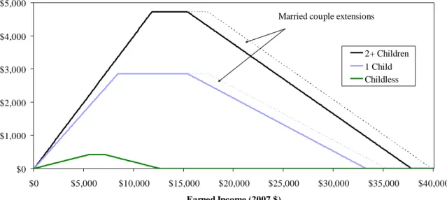
    The EITC is a refundable tax credit that was introduced in the tax code in 1975.  The credit is targeted at  low to moderate income working families, and eligibility for the credit depends on the taxpayer’s earned  income (or in some cases adjusted gross income), and the number of qualifying children who meet  certain age, relationship and residency tests.  The taxpayer must have positive earned income, defined  as wage and salary income, business self‐employment income, and farm self‐employment income.  Further, the taxpayer must have adjusted gross income and earned income below a specified amount (in  2007, the maximum allowable income for a taxpayer with two or more children is $37,783).  There are  separate tax schedules by family size—a small credit for childless taxpayers, one for taxpayers with one  child, and another (more generous payment) for taxpayers with two more children.2     

  The total tax cost of the EITC consists of two components. The pure tax expenditure is the  amount by which the EITC reduces the amount of taxes owed. Because the EITC is refundable, however,  there is also the outlay component—taxpayers receive a tax refund when the EITC exceeds their taxes  owed. The outlay component is large: in 2004 the total tax cost of the EITC was $40 billon with a pure  tax expenditure of $5 billion and an outlay of $35 billion. For the purposes of this paper and the analysis  of the EITC, we are considering the total tax cost (tax expenditure plus outlay) as the relevant object of  study.       Each of the credit schedules (for no children, one child, two or more children) consists of three  regions. At the lowest levels of earnings, in the phase‐in region, the EITC is equal to earnings times the 

subsidy (or phase‐in) rate.  In tax year 2007, the subsidy rate of the EITC is 34 percent for taxpayers with  one child, 40 percent for taxpayers with two or more children, and 7.65 percent for childless taxpayers.   Following the phase‐in, there is a relatively small range of earnings—in the flat region—where the family 

 A "qualifying child" for the EITC must be under age 19 (or 24 if a full‐time student) or permanently disabled and residing with  the taxpayer for more than half the year.

3

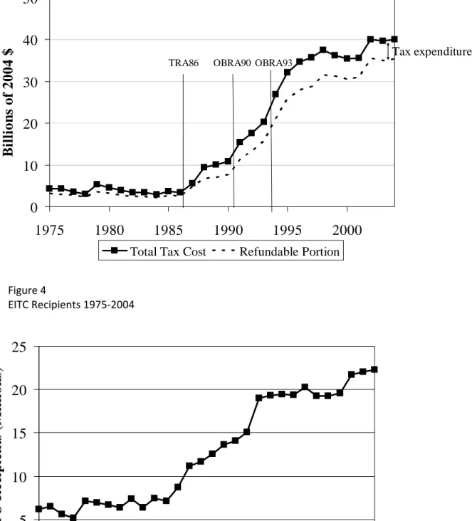
receives the maximum credit. In 2007, the maximum credit is $2,853 for one child, $4,716 for two or  more children, and $428 for childless filers.  Finally, for earnings above the flat region—in the phase‐out  region—the credit is reduced at the phase‐out rate (about 16 for one child, 21 percent for two or more  children, and 7.65 for childless). The flat and phase‐out regions of the EITC are extended by $2,000 for  married filers in 2007; this is the only aspect of the credit schedule which varies by filing status.  Overall,  the 2007 EITC schedule is traced out in Figure 1.  This illustrates the quite modest size (relatively) of the  credit for childless taxpayers, and the large range of the phase‐out region covering earnings well beyond  the lowest income taxpayers. For comparison, 2006 median family income (not earnings) was $48,201  for all households and $31,818 among female headed households (DeNavas‐Walt et al 2007).      Table 1 summarizes the parameters of the EITC over the history of the program. Originally, in  1975, the EITC was a modest program aimed at offsetting the social security payroll tax for low‐income  families with children.  It was the outcome of a vigorous policy debate surrounding the efficacy of a  Negative Income Tax (NIT) as a means of reducing poverty.  The concern was that the NIT—which  guarantees a minimum standard of living to everyone—would discourage labor market activity as it is  gradually phased out. Ultimately the EITC was born out of a desire to reward work.  Subsequently, the  EITC expanded substantially through tax acts in 1986, 1990 and 1993.  As part of the Tax Reform Act of  1986 (TRA86), by 1988 taxpayers with incomes between $11,000 and $18,576 became eligible for the  credit and faced its phase‐out marginal tax rate for the first time. The largest single expansion, as part of  the Omnibus Reconciliation Act of 1993 (OBRA93), led to a large increase in the subsidy rate (and  maximum credit) along with a modest increase in the phase‐out rate. OBRA93 also introduced the credit  for childless filers. Figure 2 shows the EITC credit in real terms before and after each of the three key tax  acts (for families with children) and highlights the dramatic expansion of the credit over time, as well as  its effects on the families of different sizes.      These expansions have led to a dramatic increase in the total cost of the EITC.  Figure 3 shows  the total real outlay (refundable portion) and the total real tax cost of the EITC from 1975 to 2004, with  the difference being the pure tax expenditure. The figure clearly shows the rising expenditures  associated with the 1986, 1990, and 1993 tax acts.  Importantly, between 1990 and 1996 the program  more than doubled in real terms. Figure 4 shows that much of this increase in costs is driven by the  increase in the number of recipients—in 1995, 19 million filers received the EITC, 160% more than ten 

4 years earlier.3 Figure 3 also shows that the vast majority of the total tax cost—throughout the history of  the EITC—derives from the refundable portion of the credit rather than the pure tax expenditure.      Given that the EITC primarily takes the form of a direct outlay, it is useful to outline the tradeoffs  involved in transferring dollars through the tax system. The main advantage of redistribution through  the tax system is the low administrative costs enabled by the use of income information already  collected for tax purposes.  This argument was made as early as 1962 by Milton Friedman in arguing for  a negative income tax as the means of assisting low‐income people (see also the discussion in Liebman  1998).  Indeed, administrative costs amount to an estimated 0.5 percent of EITC benefits (IRS 2003).   This compares to about 16 percent of the budget for traditional transfer programs (Green Book 2004).   Further, there is less "stigma" associated with benefits received through the tax system than through  welfare agencies, due to the lack of a separate application and “inquisition” by caseworkers. The net  effect of the lower stigma is to increase take‐up and well‐being of those eligible for assistance.  A  disadvantage of administering benefits through the tax system is that the IRS is not as well suited to  monitor compliance with the eligibility criteria other than income—such as verifying qualifying children,  especially with intergenerational families and non‐custodial parents. In addition, the “lump sum” nature  of the EITC may require costly consumption smoothing for families. Finally, current year EITC is tied to  prior year income, which may lead to inefficiencies given that employment and living arrangements  change frequently for the low income population.    

3.

Who

Gets

the

EITC?

Distributional

Analysis

under

Current

Law

 At the same time as the federal EITC was expanding, many states introduced "add on" credits as part of their state income tax  schedule. As of January 2006, a total of nineteen states and the District of Columbia have state EITC’s, typically structuring their  credits as a share of the federal credit, varying between 5 percent in Illinois to more than 40 percent in Minnesota and  Wisconsin (Nagle and Johnson 2006). The cost of the state EITCs is estimated to be $1.5 billion (Okwuje and Johnson 2006).

5 status, and EITC credit range.  The number of EITC returns is about evenly split between those with one  child versus two or more children (8.4 million with one child and 9.2 million with two or more children).  Owing to the more generous credit for larger families, however, filers with two or more children receive  62 percent of the total tax cost while those with one child receive 36 percent of expenditures. Childless  recipients represent 21 percent of all EITC recipients—numbering 4.7 million in 2004—but only 2  percent of the total tax cost. Table 2 also shows that head of household filers (unmarried with children)  represent 53 percent of EITC returns and 65 percent of tax expenditures. Married couples filing jointly  make up a quarter of recipients and tax costs; the remaining quarter of recipients and 10 percent of tax  costs go to single filers. This disproportionate share of unmarried filers among the EITC population  reflects the higher eligibility rates—due to lower earnings and income—of single women with children.  The average EITC benefit (refundable and nonrefundable) per recipient is $218 for those with no EITC  qualified children, $1,715 for those with one child, and $2,693 for those with two or more children.     The distribution the credit dollars and recipients by EITC region—phase‐in, flat, and phase‐out— is also presented in Table 2.  This distribution effectively determines the net labor supply effect of the  EITC.  About one quarter of EITC returns and expenditures go to filers in the phase‐in or subsidy region.   About 19 percent of recipients and 29 percent of the total tax cost is for recipients in the flat region, and  fully 54 percent of recipients and 48 percent of the total tax cost is for recipients in the phase‐out  region. This shows that more than three‐quarters of recipients have earnings in the flat and phase‐out  range where negative hours of work incentives are predicted (work incentives are discussed more fully  in the next section).  Married couple filers are even more likely to have income outside the phase‐in  range: tabulations by filing status and credit region (not in Table 2) show that about 84 percent of  married EITC recipients have income in the flat or phase‐out regions compared to 70 percent among  head of household filers.     We extend this profile of EITC recipients by examining the distribution of tax filers and EITC  recipients by ranges and deciles of cash income, in Table 3.4  By design, the benefits of the EITC are  concentrated at the bottom of the income distribution.  About 35 percent of the EITC total tax cost goes  to filers in the 3rd cash income decile ($11,163 to $17,100 in 2004).  About a quarter of the tax cost is in 

 Cash income is constructed as AGI less state and local tax refunds, plus deductions for IRA, student loan interest, alimony paid,   tuition & fees, health savings account, one‐half of self‐employment tax, penalty on early withdrawal of saving, self‐employed  health insurance, medical savings account, Keogh, tax‐exempt interest, non‐taxable social security benefits, and other income  (if positive). Note that this excludes non‐taxable income such as public assistance benefits. Finally, we follow the common  practice of dropping those with negative income when presenting means of the bottom decile (but they are included in the  totals). Those with negative income account for less than 1 percent of returns (weighted).

6

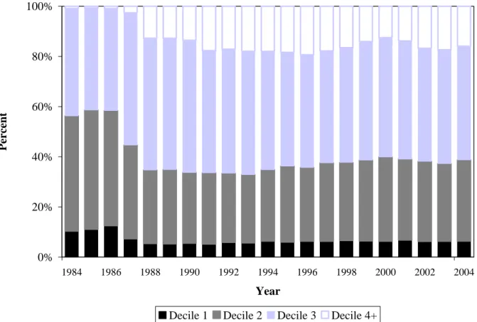
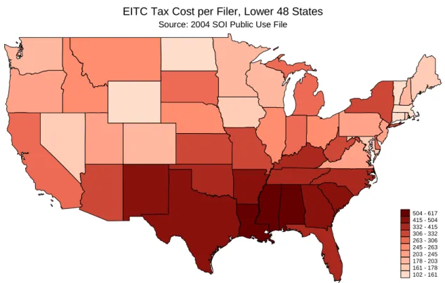
the each of the 2nd and 4th cash income deciles (with $5,302‐$11,162 and $17,101‐$23,570 respectively).   Notably, a somewhat smaller amount, 5 percent, goes to the very lowest cash income decile (below  $5,301) where there are fewer eligible filers.  The remaining 12 percent of the tax cost is above the 4th  decile (almost all of that is in the 5th decile).    These distributional impacts across income deciles are highlighted in Figure 5. The top panel of  the figure presents the distribution of EITC costs and recipients by income decline, as previously shown  in Table 3. Overall, it may be surprising that the EITC benefits taxfilers all the way into the fifth decile of  the income distribution where incomes range from $23,570 to $31,650 (and does not benefit taxpayers  in the bottom income decile).  In Panel B, we define the income deciles based on “family size  equivalent” income measures. In particular, we follow the practice of CBO by dividing family income by  the square root of family size for the purpose of ranking families. Using this alternative definition of  income deciles, we find that the EITC tax cost to be more concentrated in the lowest deciles—almost  three‐quarters of the tax cost are in deciles two and three. For the remainder of the paper, we return to  our original income deciles (unadjusted for family size).    The distribution of the EITC tax cost by income decile for tax years 1984 through 2004 (figure 6)  shows the benefits have shifted from the bottom decile further up the income distribution to the 4th  decile and above.  Interestingly, most of the change occurs around the expansions in TRA86, with less  dramatic effects of OBRA90 and OBRA93.    Finally, we find a distinct geographic pattern in the distribution of EITC tax expenditures (Figure  7).   This figure plots EITC expenditures per state tax‐filer for each of the 50 states (and the District of  Columbia).5  As one might expect, the per‐filer EITC tax cost is highest in the poorest states (Louisiana  $617, Mississippi $616, District of Columbia $570, Alabama $505, Georgia $504). The tax cost per filer  tends to be lowest in richer states (Vermont $121, Hawaii $139, Massachusetts $159, Connecticut $161,  Maryland $168) as well as states that have fewer filing units with children (Wyoming $102, North Dakota  $152).     

4.

Behavioral

Effects

of

the

EITC

5

Note that this is a measure of the tax benefits per state not state tax burdens. The burden is faced by all taxpayers, not just  state residents.

7

A primary motivation for recent expansions of the EITC is to reward the values of “work and family.”  In  this section, we discuss the incentives created by the credit for work and family formation, and review  the empirical evidence. 

Labor Supply Incentives  

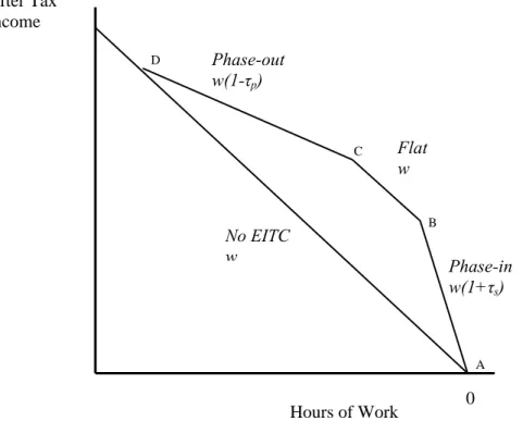
A key design feature of the EITC and what distinguishes is from traditional income support programs, is  that the EITC is only provided to working families and in so doing promotes work. However, the  additional tax from the phase‐out rate is expected to reduce work among those already in the labor  force. Thus the overall prediction is an increase in the extensive margin and a reduction in the intensive  margin of labor supply.      Consider first families with one parent or one potential earner. Figure 8 presents a stylized  budget constraint, plotting hours worked on the horizontal axis against after tax income on the vertical  axis, ignoring for simplicity all other features of the tax‐transfer system outside the EITC. In the absence  of the EITC, the taxpayer earns a gross wage w for each hour worked—hence the no‐EITC budget  constraint is given by segment AD, with slope w. The EITC alters the budget constraint to ABCD.  In the  phase‐in region (AB), the EITC acts as a pure wage subsidy and increases the net wage from w to 

(1

)

w

+

τ

τ

τ

τ

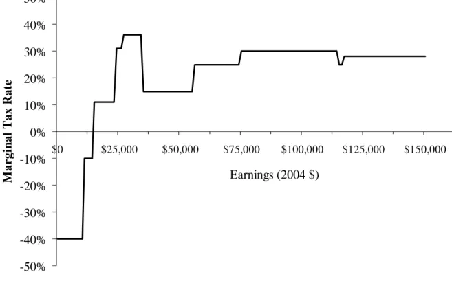
8 expanded or introduced.  If she is in the phase‐in region, the EITC leads to an ambiguous impact on  hours worked due to the negative income effect and positive substitution effect. In the flat region and  phase‐out regions, however, the EITC is expected to reduce hours through a negative income effect, and  additionally in the phase‐out, a negative substitution effect. Moreover, the phase‐out of the credit alters  the budget set in such a way that some taxpayers with incomes beyond the phase‐out region may  choose to reduce their hours of work and take advantage of the credit. In practice most EITC recipients  have income beyond the phase‐in: for example in 2004 about 70 percent of single filers and 84 of  married filers receiving the EITC have earnings in the flat or phase‐out region of the credit (more on this  below).  Thus the expectation is that the EITC will reduce the number of hours worked by most eligible  single taxpayers already in the labor force.      These labor supply incentives are substantial.  Eissa and Hoynes (2006b) show that in 2004 a  single filer with one child earning $10 per hour considering part‐time work faces a average tax rate of  negative 10 percent (a subsidy), compared to a tax rate of 15 percent without the EITC—a reduction in  the participation tax of 25 percentage points. Further, recipients with incomes in the phase‐out range  face marginal tax rates that are high by federal income tax standards.  NBER TAXSIM‐simulated marginal  tax rates on 2004 earnings for a single filer with two children are shown in Figure 9.  For these  simulations, we assume that the family only has earned income, takes the standard deduction, and the  tax calculation ignores state income taxes, the AMT, and the payroll tax. This figure shows that the  marginal tax rates in the phase‐out are higher than those experienced by taxpayers at far greater  earnings.       In contrast to the predictions for single women, the EITC is expected to reduce the participation  and hours worked of most eligible married women.  This occurs also because the credit is based on  family earnings and income. Suppose family labor supply follows a sequential model, with the husband  as the primary earner and the wife as the secondary earner.  In this model, the effect of the credit on  the labor supply of primary earners is the same as that of single taxpayers—incentives to participate in  the labor market strengthen unambiguously while hours of work incentives are ambiguous, though likely  negative given the distribution of taxpayer income along the EITC schedule.      The impact of the EITC on secondary earners is more complicated because it depends on the  earnings of the primary earner.  Assume for simplicity that the husband is the primary earner, and  further that his earnings place the family in the phase‐out range. The family receives the credit if the 

9 wife remains out of the labor force, but the credit amount will decrease with each dollar earned if she  enters the labor market. In the phase‐out range, therefore, the EITC unambiguously reduces hours  worked and participation, by raising family after‐tax income and reducing the net‐of‐tax wage.  If the  husband’s earnings place the family in the flat region, the credit unambiguously lowers labor‐market  participation and hours worked by married women (through a pure income effect).  Of course, it is also  possible for the wife’s work effort to increase the family’s credit if the husband’s earnings are in the  subsidy region (up to $8,390 or $11,790 in 2007 depending on the number of children), but very few  married couples are likely to have incomes in this range. Given the distribution of income, it is unlikely  the EITC will have any positive effect on the intensive or extensive margins of labor supply of married  women.   

Empirical Evidence on Labor Supply   

A large body of work has examined the behavioral responses to the EITC. Here we touch on the major  findings in the literature; those interested in a more comprehensive review should see Hotz and Scholz  (2003) and Eissa and Hoynes (2006b).    Much of the empirical literature focuses on estimating the incentive effects on labor supply for  single mothers. That work shows consistently that the EITC leads to significant increases in employment  (extensive margin) but there is little evidence that the EITC leads to a reduction in labor supply for those  in the labor market (intensive margin). Perhaps most striking about these findings is their consistency  across different empirical methods—including quasi‐experimental methods (Eissa and Liebman 1996,  Ellwood 2000, Hotz et al 2002, Meyer and Rosenbaum 2000, and Rothstein 2007) and more structural  methods (Dickert et al 1995 and Meyer and Rosenbaum 2001)—as well as different EITC expansions.      Evaluations of the large federal expansions in the credit in 1986, 1990, and 1993 typically use  difference‐in‐difference models and compare changes for a treated group (e.g. single mothers with  children) to a control group (e.g. single mothers without children). The control group is introduced to  control for other factors that may be contemporaneous with the policy changes. The EITC design and  expansions suggest a number of possible strategies—such as comparing women with different family  sizes (presence and number of children), marital status, earnings or education levels—for identifying  labor supply responses.  These models seem to work well and provide robust estimates for the impact of  the EITC on participation, but may be less well suited for estimating the impacts on hours worked.   Analyzing the determinants of hours worked is more complicated due to the changes in the composition 

10 of the working sample and selection into work more generally.        To illustrate the findings from the difference‐in‐difference literature, Figure 10 presents annual  employment rates for women by marital status and presence of children for 1983‐2006.6 The figure  shows the dramatic increase in employment rates for single women with children compared to single  women without children. Most of this change occurred between 1992 and 1999 where employment  rates for single women with children increased by 16 percentage points.  This is during the period of the  largest expansion in the EITC due to OBRA 1993.  Over this same period, there was little change in  employment rates of single women without children.  Others have shown that the groups with the most  to gain from EITC expansions (e.g, women with lower wages, lower education levels, more children, and  single women) experienced larger gains in employment rates (Ellwood 2000, Meyer and Rosenbaum  2000, Rothstein 2007).      Eissa and Liebman (1996) find that the 1986 expansion of the EITC led to a 2.8 percentage point  increase in employment rates (relative to the base of 74.2) for single mothers.  Meyer and Rosenbaum  (2001) find that 60 percent of the 8.7 percentage point increase in annual employment single mothers  between 1984 and 1996 is due to the EITC.  They find that a smaller amount, 35 percent of the increase  in employment between 1992 and 1996 is due to the EITC (with the remainder due to welfare reform  and other changes). The range of the implied employment elasticity with respect to net income across  all studies is quite narrow—between 0.69 and 1.16 (Hotz and Scholz 2003).     A few papers examine the impact of EITC on hours for single mothers already in the labor  market (Eissa and Liebman 1996, Meyer and Rosenbaum 1999, Rothstein 2007). In sharp contrast to the  findings above, however, there is little evidence consistent with the expected negative intensive margin  effect. Some studies estimate positive effects, some negative, and most are statistically insignificant.  Another source of evidence builds on the prediction from labor supply theory that taxpayers should be  bunched at the kinks in the EITC schedule (and should be less present at the end of the EITC schedule).  Liebman (1998) and Saez (2002b) use tax return data and find no evidence of consistent with these  predictions.   

 These tabulations are calculated using the 1984‐2007 March Current Population Surveys. The sample includes all women aged  19‐44 who are not in school or disabled. We also drop the relatively small number of women who report working positive hours  but have zero earnings or report positive earnings but zero hours. For these calculations, employment is defined by any work  over the (prior) calendar year.   

11 This finding—of a significant extensive margin effect but no intensive margin effect—is  consistent with the current consensus that intensive labor supply elasticities are relatively small. It might  also be that EITC recipients are not fully aware of the structure of the EITC schedule. They receive the  EITC as lump sum payment with their tax return and have few opportunities to learn about the schedule.       There are fewer studies on the incentive effects for married couples; but the available evidence  is consistent with the theoretical expectations.  Eissa and Hoynes (2004) and Ellwood (2000) find that  EITC expansions led to modest reductions in employment rates of married women. Eissa and Hoynes  (2004), for example, compare married mothers to married women without children and find that the  1993 EITC expansion led to a one percentage point reduction in the participation rate of married  mothers.  Eissa and Hoynes (2006a) use instrumental variables methods and find that EITC expansions  from 1984‐1996 led to a small—one to four percent—decrease in annual hours for working married  women with children. Heim (2005) estimates a structural model of family labor supply and finds similar  impacts on hours worked of married women (yet he finds no impact of the EITC on employment of  married women).    

Tax Cost of Marriage 

Because the EITC is based on family income and because the same credit schedule applies to all  taxpayers with children regardless of marital status7, the EITC is not neutral with respect to marriage. By  non‐marriage neutrality, it is meant that the credit for a married couple differs from that for two  unmarried individuals with the same total income and family size.  Marriage non‐neutrality is not unique  to the EITC, however.  Both federal and state taxes (Feenberg and Rosen 1995) and traditional transfer  programs generally are not marriage neutral.  Other, less‐prominent, provisions in the tax code that  generate marriage non‐neutrality include those related to the child‐care tax credit.  Together these  features operate to tax marriage in some cases and subsidize it in other cases.      To see how this works, consider an extreme case: a married couple in 2004 with four children,  each earning $14,000 for a total of $28,000.  Their credit is $1,570.  If they divorce and each takes 2  children, their credit jumps to $8,600.   Their marriage costs them over $7,000 in lost earned income  credit (or 25 percent of their joint income).   On the other hand, very low income people may gain from  marriage.  Consider a single parent with two children who earns $5,000 gets and EITC of $2000.   If she 

7_{To offset the marriage penalty associated with the EITC, EGGTRA expanded the size of the flat credit for married}  filers 

12 marries someone earning $10,000, for a combined income, their credit jumps to $4100 (for a marriage  bonus of $2,100, or 14 percent of their joint income).    In tax year 1999 [need to update], approximately 48 percent of couples filing a joint federal tax  return faced a marriage penalty averaging $1141, while 41 percent received a marriage bonus averaging  $1274 (Bull et al 1999). These modest overall penalties mask substantial heterogeneity in the  population. Penalized married taxpayers with less than $20,000 earned income face an average  marriage penalty of 8 percent of income. A significant share of marriage penalties and subsidies incurred  by lower income families is caused by the loss of the EITC (CBO 1997).      Relatively little empirical work has examined the impact of the combined tax and transfer  system on the family (see for example, Dickert‐Conlin and Houser ‐DCH‐1998, Eissa and Hoynes –EH‐  2000a,b).   Consistent with the work on traditional welfare programs, DCH find no effect of taxes and  transfers on the decision of females to become heads of household (through out‐of‐wedlock birth or  divorce).  Eissa and Hoynes (2000a) document the changes to the tax consequence of marriage from  1984 to 1997, and show it declined following the flattening of the federal tax schedule in 1986 but then  subsequently increase in the period after.  They use this time variation in the tax consequence of  marriage, augmented with the impact of welfare (ADFC/Food Stamps/Medicaid) to examine the impact  on the propensity of women to be married, and find a small impact of the tax‐transfer system on  marriage (EH 2000b).   On balance, the evidence suggests the tax consequence of marriage has a minor  impact on behavior and raises mostly distributional concerns.     

Should the Tax System be Neutral with Respect to Marriage? 

While nearly 60 provisions of the federal income tax code alter tax liability by marital status (GAO,  1997), it is primarily the combination of a progressive income tax schedule and taxation on the basis of  total family income that generates marriage non‐neutrality.  Although marriage neutrality of the tax  code has been espoused by some, it is not at all clear that the tax system should treat marriage  neutrally.  On the one hand, the notion of horizontal equity suggests that marriage should be taxed  because couples benefit from economies of scale deriving from sharing resources.  The benefits of  economies of scale accrue to any group of individuals residing together, however, and are not taxed  generally if they accrue to cohabiting couples, adult children living with parents, or group‐home  residents. On the other hand, marriage confers social benefits primarily in the form of child wellbeing.   

13 To the extent that the relationship between marriage and child well‐being is causal, and to the  extent that individual marriage decisions ignore the social benefits, a strong argument for government  intervention emerges. Here, the tax code should subsidize marriage. In addition, the strong correlation  between poverty and single‐parent families suggests that marriage may be viewed as a cost‐effective  poverty alleviation policy.      The 2001 and 2003 tax cuts lowered marriage penalties by adjusting the size of the maximum  EITC credit region for married couples, and by making the standard deduction and 15 percent bracket  twice the size as for a single taxpayer.  Making these permanent is likely to be very costly, however,  about $130 billion dollars over the 2008‐2017 budget window (Tax Policy Center, 2007).     

5.

Hypothetical

Reforms

to

the

EITC

Other simulations that are of interest to the wider tax expenditures project are removing the “AMT patch” and eliminating the  2001 and 2003 tax cuts. We have examined these scenarios and show that they lead to no significant changes for the EITC. Thus  we have chosen to not present them here although they are available on request. In an effort to lesson the marriage penalty,  the 2001 tax act did expand the flat and phase‐out regions of the EITC for married couples (as illustrated in Figure 1 and  specified in the notes to Table 1). In practice, these changes were modest in size and impact.

14 suggestive, however, since a full blown analysis with parametric utility functions and social welfare  weights is beyond the scope of this paper (see Liebman 2002 for such an analysis).   We defer discussion  of “marginal reforms”—Panels E and F—to Section 6, in which we carry out a welfare evaluation of  different EITC phase‐out rates.      Our evaluation here is based on the 2004 SOI Public Use Tax Data used to profile the EITC  population.  Using those data and the NBER’s TAXSIM model, we recalculate each taxfiler’s tax liability,  marginal tax rate under the alternative EITC policies, and aggregate to get the number of recipients and  total cost9.  More precisely, marginal and average tax rates are defined for each dollar of earned income,  and do not include payroll taxes (we also relax this assumption in section 6) or state income taxes.   The  simulated values are used to populate distributional tables similar to those presented above under  current law, allowing us to infer the likely distributional and efficiency consequences of each reform.      Two caveats are worth noting.   The simulations of total cost, number of recipients and  (marginal and average) tax rates are static, and so assume no change in labor supply or earnings (we  relax this assumption in Section 6).10  In addition, by using the 2004 SOI data, our results are limited to  the existing sample of filers.     We present the simulated number of EITC recipients, total EITC tax cost, and distribution of the  EITC tax cost by number of children, filing status, and cash income decile under current law and the  alternative policies in Table 511. We compare marginal and average tax rates under current and the  alternative policies in Table 6.  Below, we discuss each reform separately, considering first expansionary  reforms.    

A:  Expansionary Reform 1: Increased Subsidy Rate 

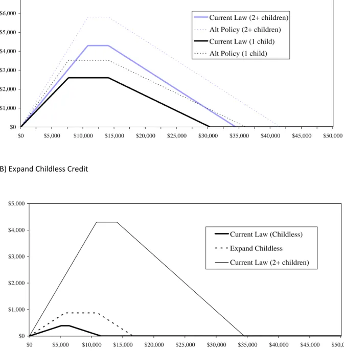
Our first expansion broadly expands the program by increasing the phase‐in rate by about one‐third:  from 34 to 46 percent for parents with one child and from 40 to 54 percent for those with two or more  children (see Figure 11a).  We hold fixed the size of the phase‐in and flat regions and so raise the 

9

Dan Feenberg was incredibly helpful in coding up all of the alternative EITC policies and making this analysis possible with  TAXSIM.

10

For married couples, we calculate the marginal tax rate for the primary earner.

11

Note that the numbers for “current law” in Table 5 differ slightly from the results presented earlier in Tables 2‐3. The current  law numbers in Table 5 use TAXSIM to calculate the EITC under current law assuming 100% take‐up. This provides the best  comparison to the simulations of the alternative policies. Our recalculation of current law shows 22.9 million recipients  (compared to 22.1 under current law) with most of these additional recipients in the childless group.

15 maximum credit to $3,487 ($5,754) for those with one child (two more children).12  It is worth noting  that this reform does not expand eligibility very far up the income distribution.  The maximum income  for the EITC rises by about 18 to 20 percent (to $35,861 and $41, 362) relative to current law.      This expansion covers an additional 2.5 million tax‐filers (11 percent) but does so at a high cost‐‐ $20 billion (or 50 percent of current law expenditures).  This expansion creates winners and no losers  (except for taxpayers who finance the additional expenditures).  Still, it is useful to note where the  dollars flow and how that changes with the alternative policy.  The distribution of the tax cost seems to  vary little by number of children and filing status, though it does benefit taxpayers with children  (especially with more than one child) and joint filers relative to head of household and single filers.  This  reform, on the other hand, transfers most of the dollars to taxfilers with higher incomes. This occurs  both across EITC regions and across the cash‐income distribution. Essentially all the benefits accrue to  tax‐filers in the phase out region—who under current law receive 49.4 percent of the dollars and under  the expanded program end up with 52.1 percent.  Those who gain most have income in the 5th and 6th  deciles of the distribution (above $23,570).         In addition to the distribution of benefits, we examine the impact of EITC reforms on average  and marginal tax rates.  Simulations, presented in Table 6, show this  expansion reduces average tax  rates (calculated as tax liability relative to earned income) for most for head of household filers (by ‐4.7  percentage points), and for taxpayers in the flat region of the EITC (by ‐4.9 percentage points). The table  also breaks out the impact on newly eligible taxpayers (with incomes between the current law maximum  and $35,861 and $41,362), and shows their tax liability declines by about 1.2 percentage points.  The  cash income distribution shows all filers below the 7th decile benefit, but that the largest gains accrue to  the second and third decile (mirroring the flat region). By reducing the tax liability, this reform expands  the budget set for all eligible filers and thereby provides stronger incentives for non‐workers to enter  the labor market.  As a consequence, it creates welfare gains along that margin of labor supply.13       The EITC expansion considered here reduces marginal tax rates (higher subsidy rates) for some  recipients and raises them (higher phase‐out rates) for other recipients.  This renders the pattern of  marginal tax rates far less consistent than that of average rates (see the bottom panel of Table 6).  Head  of household and single filers face lower marginal rates, while joint filers face a slightly higher marginal 

 This policy assumes no change to the credit for the childless.   13

16 tax rate on earnings.   By income, the simulation shows marginal tax rates decline for lower‐income filers  (in the phase‐in and flat regions, and below the second decile) and rise for those with higher incomes.   Not surprisingly, newly eligible filers face a marginal rate that is nearly 15 percentage points greater  than under current law, as they enter into the phase‐out region.   These filers have income in the 5th and  6th decile of the distribution and thereby explain the observed rise in marginal tax rates at those points.  Applying a traditional Harberger analysis suggests welfare losses on balance from the marginal rate  changes because the increases hit a thicker part of the income distribution.  This is especially the case if  the elasticity of hours worked with respect to the tax rate increases with income.    

B:   Expansionary reform 2: Increase Childless Adult EITC 

Our second expansionary reform is based on the recent proposal by the U.S. House Ways and Means  Committee to expand the EITC for childless filers (the Rangel proposal).  The proposal doubles the  subsidy rate (to 15.3 percent) to cover fully the Social Security and Medicare payroll tax rate (and  doubles the maximum credit), expands the size of the flat region, and doubles the phase‐out rate to  15.3 percent.  This reform expands eligibility to those with incomes up to $15,998 (from its current‐law  level of $11,490).    Figure 11(b) illustrates this reform and shows it to be a relatively modest expansion. .  It is  simulated to cover an additional 3.3million taxfilers (14 percent) and cost about 2.8 billion per year (7  percent over current law).   The distribution of the EITC tax cost changes in predicable ways.  More  benefits go to single filers and to filers with no children, but also to the phase‐in and (mainly) flat regions  (relative to phase‐out region).  Expanding the childless adult credit reduces average tax rates for single  filers (by 0.6 percentage points) and across the EITC distribution. More precisely, newly eligible  recipients see a decline of 0.7 percentage points in their average rates.  Evidence on the behavioral  responses of (less‐skilled) childless adults is limited, but inference from standard labor supply and tax  work generally suggests small elasticities (cites).   In work that does not incorporate income taxes, Juhn  (1992) finds substantial declines in labor market participation by less‐skilled men in the 1970s and 1980s  in response to deteriorating wage opportunities.  If is therefore possible that this reform will generate  some labor supply and efficiency gains.     C:   Universal Reforms  Our second reform makes the credit more “universal” by extending substantially the reach of the phase‐ out region up the income distribution.  That is accomplished by reducing the phase‐out rate from the 

17 15.98 (21.06) percent for families with one child (two or more children) under current law to 5.33 (7.02)  percent, respectively.  Static simulations show this expansion is projected to add $27 billion to the total  annual cost of the EITC and cover an additional 12.5 million tax‐filing units (Table 5).  Because of the  scale of this expansion, illustrated in Figure 12(a), we also consider a version that requires no additional  revenues.  The revenue‐neutral expansion is paid for by reducing the maximum credit (and phase‐in  rate) by 30 percent, as we show in Figure 12(b).      The revenue‐neutral reform is projected to cover 7.3 million (or 32 percent) more taxfilers.   Although this reform costs essentially the same as current law (by design), it has dramatic distributional  consequences.  In relative terms, the credit flows away from unmarried parents (who have lower  incomes in general) and towards married couples—who now receive 30.7 percent instead of 24.8  percent of the total benefits.  In addition, the credit flows away from tax‐filers in lower cash‐income  deciles to those in higher income deciles.  About 70.5 percent of credit dollars go to filers in the bottom  4 deciles (with income below $23,570) under the revenue‐neutral reform, down from 89.7 percent  under current law.      The impact of these redirected benefits on tax liability and average tax rates is stark.  Tax liability  rises everywhere along the EITC schedule except for those who are newly eligible.  The 7 million newly‐ eligible filers get a 1.5 percentage point reduction in their average tax rate.  On a finer level, the  distribution of average tax rate by cash income shows the revenue‐neutral expansion of the credit  benefits taxpayers above the 4th decile at the expense of all those with lower income.  This  redistribution comes at a cost for newly eligible taxpayers, however: higher marginal tax rates on hours  worked between the 6th and 8th deciles of the cash income distribution.   In fact, very low‐cash income  recipients also face higher marginal rates (as the subsidy rate is reduced).  Any negative distortion to  labor supply caused by these higher marginal rates is offset, however, by lower marginal rates (by 2 to  3.9 percentage points) for taxfilers right below the middle (in the 3rd, 4th and 5th income deciles) of the  distribution.  The efficiency consequences of this reform are therefore difficult to characterize, and  ultimately depends as well on the relative size of the elasticity of hours worked across the cash‐income  distribution and the shares of income facing higher as opposed to lower rates.      D:   Targeted Reforms  Our final set of large reforms target the credit by curtailing substantially the reach of the phase‐out  region.  That is accomplished by raising sharply the phase‐out rate from the 15.98 (21.06) percent for 

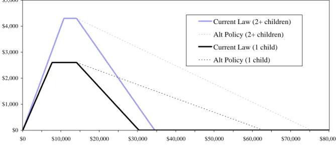
18 families with one child (two or more children) under current law to 47.94 (63.18) percent respectively  (see Figure 13a).  These rates might seem entirely unrealistic, but we note they are quite modest for  traditional welfare programs (e.g. AFDC/TANF).  The net impact is to render ineligible taxfilers with one  child and incomes between $19,472 and $30,338 ($20,846 and $34,458 for two or more children).  Static  simulations show this contraction of the EITC saves the federal government $13.4 billion annually, and  eliminates 6.8 million tax‐filing units from the program (Table 5).   The revenue‐neutral version of this  reform, illustrated in Figure 13b, redistributes the tax‐revenue savings to a higher subsidy rate and  thereby a higher maximum credit (by about one‐third its current law level).  The specific parameters are  also presented in Panel D of Table 4.      On net, the revenue‐neutral targeted EITC reform eliminates 5.4 million recipients (a decline of  about 23 percent), who are more likely to be joint filers.  Therefore, we observe redistribution from joint  filers (who have higher incomes) to single and (mainly) head of household filers.  There is very little  redistribution between parents and childless adults in this reform.  To the extent that joint filers have  more children than head of household filers, there is possible residual redistribution to childless adults.  Along the EITC schedule and cash‐income distribution, the credit flows are as expected—from  the  phase‐out to regions below—and from the 4th decile to deciles below.  In fact, this reform transfers 88.7  percent of the credit to filers with incomes at or below the 3rd decile (compared to 66.9 percent under  current law and 49.6 under the comparable universal reform).   Figure 14 illustrates further the different  distribution of benefits under current law, and each reform of the revenue‐neutral reforms (universal  and targeted).      The targeted reforms reverse the relationship between average and marginal rates we observe  for the universal reforms.  Average rates fall for recipients in the phase‐in and flat regions (and those  with incomes below the 3rd deciles) at the expense of those no longer eligible for the EITC (and with  higher incomes).  One impact of this reform is stronger incentives for non‐workers to enter the labor  market: average tax rates decline by 4.7 percentage points for entrants into the flat region; and as a  results welfare gains along the extensive margin.    Marginal tax rate changes, on the other hand, suggest substantial distortions to taxfilers in the  phase‐out region (where the increase in the MTR is fully 11 percentage points).   These are offset,  however, by the lower marginal rates that newly ineligible filers now face –on the order of 15  percentage points.  Along the cash‐income distribution, marginal rates fall for everyone except those in 

19

the 3rd and 4th deciles—who face 6.6 to 6.9 percentage point higher marginal tax rates.  Distortions to  hours worked for some are therefore offset by better incentives for others.  This pattern again  complicates somewhat the inference about the potential efficiency effects.   Thought it seems  reasonable to conclude that with elasticities that are larger on the extensive margin compared to the  intensive margin, this reform has the potential to yield efficiency gains compared to current law.  

6.

Efficiency

Impacts

of

the

EITC

 Saez shows that the optimal program is instead a classical Negative Income Tax program, with a substantial income  guarantee that is phased out a high rate. 

20 federal income tax changes not just the EITC) and show that each had different effects on tax rates along  the intensive and extensive margins.  The 1993 expansion, for example, reduced the tax rates on labor  force participation, but increased the marginal tax rates on hours worked for most workers.  The authors  show that conflating these two tax rates in welfare analysis can be fundamentally misleading.  For tax  reforms that change average tax rates differently than marginal tax rates (such as the 1993 expansion of  the EITC), ignoring the participation margin can lead to even the wrong sign of the welfare effect.   

Welfare Analysis of the EITC for Single Mothers  

In this section, we apply EKK to evaluate the efficiency effects of “small” reforms of the EITC.  Arguably,  the EITC is unlikely to be overhauled in a major way, so this approach is more relevant for understanding  the efficiency consequence of feasible reforms.  Another advantage of examining small reforms is their  simplicity and transparency.  Larger reforms, such as those examined above, generate first‐order labor  supply and revenue effects; so that a full analysis of the welfare effect of the reforms would have to  reflect the externalities created by changes in government revenue.  Here, we avoid the need to specify  utility functions or estimate (or calibrate) utility parameters, and the fixed costs of work that generate  discrete responses along the extensive margin.    To simplify the analysis further, we focus our welfare analysis on single parents (head of  household filers), who represent the largest group of recipients—accounting for about 65 percent of  EITC recipients and dollars.  This is also the group where discrete responses have been shown to be  especially important.    EKK show the marginal deadweight burden of tax reform is given by the effect on government  revenue from behavioral responses, where the behavioral revenue effect is related to the two different  margins of labor supply response.  The first effect captures the revenue effect from the change in the  optimal hours of work for those who are working.  The second effect captures the effect on revenue  brought about by the tax‐induced change in labor force participation.  While the second effect on  efficiency is related to the tax rate on labor force participation, the efficiency effect from changed  working hours depends on the tax burden on the last dollar earned.    A full description of our simulation approach and the EKK deadweight loss formula is presented  in an appendix.   We review only the basic approach here.  We start by creating a sample of single  parents from the Current Population Survey (CPS).  The CPS is better suited for this analysis because we 

21 are explicitly interested in the participation response, and because the data include potentially eligible  single parents who do not work or who do not file tax returns.  For each sample member, we estimate a  likelihood of labor market participation and potential earnings conditional on working, based on  exogenous characteristics.  This allows us to impute their earned income credit, and more generally  their net tax liability.  To be consistent and to avoid the problem of endogenous earnings and tax rates,  we use imputed earnings for workers as well.  Third, we use predicted earnings to simulate individual  marginal and average tax rates under current law and under the marginal reforms. Finally, we calculate  welfare effects based on imputed tax rates and assumed elasticities—as in equation (23) in EKK.       Tax rates are based on the NBER TAXSIM model ‐augmented by a simple welfare benefit  calculator, and therefore account for both the tax and the transfer systems.  Our measures of effective  tax rates include federal and state taxes, payroll taxes and public assistance (cash, Food Stamps and  Medicaid).15  Welfare benefits are based on each person’s state of residence and on the number of  dependent children, and are adjusted to account for the implicit tax rates in each program (except for  Medicaid), and for the less‐than‐100 percent take up rate (see Moffitt, 1992).      

Impacts of Small Reforms on Tax Parameters 

We consider two sets of simple “marginal” reforms to the EITC.  First, we change the phase‐out rate by  +/‐ 1 percentage point (from 15.98 percent for single mothers with 1 child and 21.06 percent for those  with two or more children).  This extends the credit to taxfilers with $31,423 and $35,476 of income  under the lower phase‐out rate, and to $29,376 and $33, 532 under the higher rate, respectively.    Second, we change the subsidy rate +/‐ 1 percentage point (from 34 and 40 percent respectively).  The  subsidy cut has a cutoff very similar to the phase‐out rate increase, allowing us to evaluate the impact of  transferring money to the same population but using different labor supply incentives. The full  parameters of these moderate EITC reforms are shown in Panels E and F of Table 4.      Phase‐out Rate  Panels A and B of Table 7a show the impact of changing the phase‐out rate on the number of recipients  and average and marginal tax rates.  Making the EITC more generous lowers the overall tax burden on  single mothers: the participation tax (benefit‐adjusted average tax) rate falls by 0.2 percentage points,  from 26.8 percent to 26.6 percent of wage income.  This decline is somewhat higher for taxpayers in the 

 We assume workers bear the full incidence of employer payroll taxes, and adjust pre‐tax wages accordingly.  This 

22 (current law) phase‐out region than for newly eligible filers, but generally of the same order of  magnitude.  Marginal tax rates decline by a similar 0.3 percent overall but show a far less systematic  pattern than participation tax rate: they fall by 0.7 percentage points for the 7.85 million EITC recipients  in the (current‐law) phase‐out region and increase by a full 10.7 percentage points for the 0.212 million  newly eligible recipients.  The average tax wedge, not reported in the table, is about 0.424 on the  extensive margin, and 0.532 on the intensive margin.  Panel B of Table 7a shows the impact of making  the EITC less generous has similar impacts (to Panel A) that are of the opposite sign.  About 240,000  taxpayers in the (current‐law) phase‐out of the EITC would lose eligibility, and face marginal tax rates  that are on average 11.3 percentage points lower than under current law.     Subsidy Rate  Panels C and D of Table 7a show the impact of changing the subsidy rate on the number of recipients,  and on average and marginal tax rates.  Reducing the subsidy rate by 1 percentage point, holding all  other parameters fixed, reduces the maximum credit (see Panel F of Table 4) and eliminates 118,000  recipients.  The smaller credit raises the overall tax burden and makes entry into the labor market less  rewarding:‐‐the overall participation tax rate (among EITC eligibles) rises by 0.6 percentage points.  Even  though the (average) marginal tax rate remains unchanged, it falls substantially for taxpayers no longer  eligible to receive the credit, by 10.3 percentage points.  Subsidizing earnings at a higher r