Working Paper 11-07
Statistics and Econometrics Series 04
April 2011
Departamento de Estadística
Universidad Carlos III de Madrid
Calle Madrid, 126
28903 Getafe (Spain)
Fax (34) 91 624-98-49
Non-parametric methods for circular-circular and circular-linear
data based on Bernstein copulas
Jose Antonio Carnicero Carreño, Michael Peter Wiper and Concepción Ausin
Abstract
We present a non-parametric approach for the estimation of the bivariate distribution of two circular variables and the modelling of the joint distribution of a circular and a linear variable. We combine nonparametric estimates of the marginal densities of the circular and linear components with the use of class of nonparametric copulas, known as empirical Bernstein copulas, to model the dependence structure. We derive the necessary conditions to obtain continuous distributions defined on the cylinder for the circular-linear model and on the torus for the circular-circular model. We illustrate these two approaches with two sets of real environmental data.
Keywords:
Bernstein polynomials, Circular distributions; Circular-Circular data; Circular-linear data; Copulas; Non-parametric estimation.Universidad Carlos III de Madrid, Department of Statistics, Facultad de Ciencias
Sociales y Jurídicas, Madrid, Spain. e-mail addresses:
[email protected]
(Jose Antonio Carnicero Carreño),
[email protected]
(Michael Peter Wiper) and
Non-parametric methods for circular-circular and circular-linear
data based on Bernstein copulas
Jose A. Carnicero, M. Concepci´
on Aus´ın and Michael P. Wiper
Departamento de Estad´ıstica
Universidad Carlos III de Madrid, Spain
Abstract
We present a non-parametric approach for the estimation of the bivariate distribution of two circular variables and the modeling of the joint distribution of a circular and a linear variable. We combine nonparametric estimates of the marginal densities of the circular and linear components with the use of class of nonparametric copulas, known as empirical Bernstein copulas, to model the dependence structure. We derive the necessary conditions to obtain continuous distributions defined on the cylinder for the circular-linear model and on the torus for the circular-circular model. We illustrate these two approaches with two sets of real environmental data.
Keywords: Bernstein polynomials, Circular distributions; Circular-Circular data; Circular-linear data; Copulas; Non-parametric estimation.
1
Introduction
Circular data arise when we measure the data in the form on angles or two dimensional orientations. Also, phenomena that are periodic in time and may be converted to angular data given a period of reference. Examples of this type of data can be obtained in many science fields such as biology (direction of movement of migrating animals), geology (directions of joints and faults), meteorology (wind directions), operation research (times of hospital admittance in the urgencies room), medicine (level of effect of a medicine between two consecutive doses).
Data of this type are usually represented as points on the circumference of an unit circle or as angles in the interval [0,2π). For modelling this type of data, different parametric models can be used such as the
Von Mises distribution, circular uniform distribution, wrapped distributions, etc., see e.g. Mardia and Jupp (1999) for a full review. However, these models are generally unimodal and symmetric and, alternatively, more flexible models have been proposed in the literature, using for example semiparametric approaches based on mixture of distributions (Mardia and Sutton, 1975) or Fourier series (Fern´andez-Dur´an, 2004) and non-parametric methods using kernels (Bai et al., 1988, Fisher, 1989) and Bernstein polynomial approximations (Carnicero et al., 2010).
Natural extensions of univariate circular distributions to the bivariate case are circular-linear distributions and circular-circular distributions. There have been a number of parametric and semiparametric approaches to analyzing distributions of this type, see e.g. Batschelet (1981), Mardia and Sutton (1978), Johnson and Wehrly (1978), Kagan et al. (1973), Mardia (1975), Jammalamadaka and Sarma (1988) and Fern´ andez-Dur´an (2007). Different tools have been developed for analyzing the relationship between this variables using regression models, see e.g. Jammalamadaka and Sarma (1993) and Gould (1969) and correlation coefficients, see e.g. Rivest (1982), Mardia (1976), Stephens (1979) and Johnson and Wehrly (1977).
Alternatively, in this paper, we develop a nonparametric approach to these types of data, where we com-bine nonparametric estimates of the marginal densities of the circular and linear components with the use of a class of nonparametric copulas, known as Bernstein copulas, to model the dependence structure. Bernstein copulas (see e.g. Pfeifer et al., 2009 and Sancetta et al., 2004) provide a very flexible and nonparametric description of the dependence among random variables and, in particular, it can be shown that any given copula can be approximated arbitrarily well by a Bernstein copula.
Along this paper, we show how circular-circular and circular-linear distributions can be constructed via empirical Bernstein copulas showing that for this type of data the generated distribution satisfy certain continuity constraints to be well behaved bivariate distributions. We have designed an algorithm which is non-parametric in all its stages. We use a non-parametric estimation of the distribution function as the linear distribution and the circular Bernstein polynomial for the circular distribution. Observe that for the empirical Bernstein copula model the dependence structure estimated with the copula function depends on the data observed. Similar to the univariate circular Bernstein polynomial (see Carnicero et al. 2010), we must impose certain restrictions in the model for constructing a well behaved bivariate distribution. We will show that these corrections preserves the uniformness of the marginal distributions.
The article is organized as follows. In Section 2, we introduce the univariate Bernstein polynomial and describe how it can be used to approximate univariate circular distributions on the circle, as described in Carnicero et al. (2010). In Section 3, we extend the situation to bivariate Bernstein polynomials and explain
how they can be used to define empirical Bernstein copulas. In Section 4, we define the circular-circular model based on Bernstein copulas and describe how to estimate it in a non-parametric way. In Section 5, we define the circular-linear model based on Bernstein copulas and describe how to estimate it in a non-parametric way. In Section 6, we illustrate these two models with environmental data and finally, we present some conclusions and possible extensions in Section 7.
2
Univariate circular Bernstein polynomial distributions
In this section, we describe how Bernstein polynomials can be used to approximate distributions defined on a closed interval and how this can be extended to circular variables using the approach proposed in Carnicero et al. (2010).
Consider a random variable,X, with finite support in [0,1] and continuous distribution function,FX(·).
This distribution function can be approximated using the Bernstein polynomial distribution of orderkwhich is defined by, Bk(x) = k X j=0 FX j k k j xj(1−x)k−j,
for 0≤x≤1. Note thatBk(x) is a distribution function and it is well known that it converges uniformly to
FX(x) as kapproaches to infinity, see e.g. see e.g. Lorentz (1986). Differentiating, the associated Bernstein
density function is given by,
bk(x) = k X j=1 FX j k −FX j−1 k β(x|j, k−j+ 1),
whereβ(x|a, b) is a beta density function given by,
β(x|a, b) = 1
B(a, b)x
a−1(1−x)b−1
,
where B(a, b) = (a−1)!(b−1)!/(a+b−1)!, for a, b,∈ N, is the beta function. Clearly, the Bernstein
polynomial distribution can be generalized for the approximation of any random variable defined on a closed interval using a simple linear transformation.
The use of Bernstein polynomials can be extended to approximate circular densities by assuming that the circle is a closed interval of size 2πas follows (see Carnicero et al., 2010). Consider a circular random
variable, Θ, with density functionfΘ(θ). Then, it is required that, fΘ(θ+ 2π) =fΘ(θ), forθ∈R, and Z 2π 0 fΘ(θ)dθ= 1.
Also, in order to define a cumulative distribution function, it is necessary to establish an origin, 0≤ν <2π, such that the cumulative distribution function fromν is,
FΘν(θ) =
Z ν+θ ν
fΘ(u)du, (1)
for 0 ≤θ < 2π. Then, rescaling onto [0,2π) and shifting the origin toν, we define the circular Bernstein polynomial density of orderkgiven by,
fkν(θ) = 1 2π k X j=1 FΘν 2πj k −FΘν 2π(j−1) k β θ 2π j, k−j+ 1 , (2) whereFν
Θ(·) is defined in (1). For this to be a strictly continuous, circular density, it is necessary that,
FΘν 2π k = 1−FΘν 2π(k−1) k . (3)
Carnicero et al. (2010) show the existence of at least one origin satisfying the previous equation. Therefore, using the ideas proposed in Vitale (1975), a natural estimator for a continuous density function,fΘ(θ) on
the interval [0,2π] would be given by, ˆ bνk(θ) = 1 2π k X j=1 ˆ FΘν 2πj k −FˆΘν 2π(j−1) k β θ 2π j, k−j+ 1 , (4) where ˆFν
Θ(θ) is the empirical distribution function relative to the originν. However, as in (3), this estimator
will only be circular if the difference,d(ν), between the first and the last weight of the beta mixture density (4) is zero, where, d(ν) = ˆFΘν 2π k + ˆFΘν 2π(k −1) k −1.
et al. (2010) propose to modify the standard Bernstein polynomial estimator (4) by averaging the first and last weights using,
ˆ fkˆν(θ) = 1 2π 1 2 ˆ Fνˆ 2π k + 1−Fˆνˆ 2π(k −1) k β θ 2π 1, k + k−1 X j=2 ˆ Fνˆ 2πj k −Fˆνˆ 2π(j−1) k β θ 2π j, k−j+ 1 + 1 2 ˆ Fˆν 2π k + 1−Fˆνˆ 2π(k−1) k β θ 2π k,1 .
It can be shown that this estimator has the same asymptotic properties as the Vitale estimator, see Carnicero et al. (2010) for further details.
3
Bivariate Bernstein copulas
In this section, we extend the univariate Bernstein polynomial to the bivariate case and show how to apply it in the construction of bivariate Bernstein copulas (see e.g. Sancetta et al., 2004), which will be the basis for the circular-linear and circular-circular models presented in the next two sections.
Consider a bivariate random variable, X, with support in [0,1]2 and continuous bivariate distribution
function,FX(·,·). This distribution function can be approximated using the bivariate Bernstein polynomial
of orderk= (k1, k2), which is defined by,
Bk(x1, x2) = k1 X j1=0 k2 X j2=0 FX j1 k1 ,j2 k2 2 Q i=1 ki ji xji i (1−xi) ki−ji.
Similar to the univariate case, it is well known thatBk(x1, x2) converges uniformly toFX(·) ask1 and k2
goes to infinity, see e.g. Lorentz (1986). The associated bivariate Bernstein density function is,
bk(x1, x2) = k1 X j1=1 k2 X j2=1 wj1j2 2 Q i=1 β(xi|ji, ki−ji+ 1), where, wj1j2=FX j 1−1 k1 ,j2−1 k2 +FX j 1 k1 , j2 k2 −FX j 1−1 k1 ,j2 k2 −FX j 1 k1 ,j2−1 k2 ,
which is the probability that an observation belongs to the regionhj1−1
k1 , j1 k1 i ×hj2−1 k2 , j2 k2 i
marginal distribution of each variable is a univariate Bernstein polynomial, Bk1(x1) =Bk(x1,1) = k1 X j1=0 FX j1 k1 ,1 k1 j1 xj1 1 (1−x1) k1−j1.
Bernstein polynomials can be used to define a class of non-parametric copulas, which are called Bernstein copulas. A bivariate copulaC(u, v) is a joint distribution on the unit square [0,1]2such that both marginals are uniformU(0,1). Sklar (1973) showed that every joint distribution,F(x, y),whose marginals are given byF1(x) andF2(y),can be written as,
F(x, y) =C(F1(x), F2(y)), (5)
for a function C that is called a copula ofF. If the marginal distributions are continuous, this copula is unique.
Conversely, given a two-dimensional copula,C(u, v), and two univariate distributions,F1(x) andF2(y),
the function (5) is a bivariate distribution function with margins F1 and F2, whose corresponding density
function is given by,
f(x, y) =c(F1(x), F2(y))f1(x)f2(y), (6)
wheref1 andf2 represent the marginal density functions andc is the density function of the copula which
is derived from (6) and is given by,
c(u, v) = f F −1 1 (u), F −1 2 (v) f1 F1−1(u) f2 F2−1(v) .
Various parametric copulas have been proposed in the literature. For example, the Gaussian copula function is defined by,
Cρ(u, v) = Φρ(Φ−1(u),Φ−1(v)),
where u, v ∈ [0,1] and Φ(·) denotes the standard, normal cumulative distribution function and Φρ(·,·) is
the distribution function of a standard, bivariate normal random variable with correlation ρ. Many other parametric families of copulas have been developed, see e.g. Nelsen (1999) for a good review.
When the dependence structure is unknown, non-parametric copulas provide a useful alternative, see e.g. Nelsen (1999). Formally, given a sample, {(x1, y1), . . . ,(xn, yn)}, from the joint distribution of (X, Y), the
(ui, vi) = ( ˆFX(xi),FˆY(yi)), for i = 1, . . . , n, where ˆFX(·) and ˆFY(·) are consistent estimators of the true
marginal distributions,FX(·) andFY(·), respectively. The transformed values now form a sample on [0,1]2.
Then, the empirical copula distribution function is defined as,
ˆ Cn(u, v) = 1 n n X i=1 I(ui≤u, vi≤v), for 1≤i≤n,1≤j ≤n.
Note that by construction, the empirical copula is a valid distribution function. However, it has marginals which are uniform only asymptotically asn→ ∞and therefore is a valid copula only asymptotically. Clearly, the empirical copula is not a smooth function. A smoothed version can be obtained via the Bernstein polynomial approximation (see e.g. Sancetta and Satchell, 2004) as follows.
Given a sample, (ui, vi) fori= 1, . . . , n, calculated by transforming the original data as above, then using
Slark’s theorem, there exists a copula which can be approximated with the empirical Bernstein copula of orderk= (k1, k2), which is defined as:
ˆ CB(u, v) = 1 n k1 X j1=0 k2 X j2=0 n X i=1 I ui ≤ j1 k1 , vi≤ j2 k2 k1 j1 uj1(1−u)k1−j1 k 2 j2 vj2(1−v)k2−j2. Clearly, using (6), the corresponding empirical Bernstein copula density is given by,
ˆ cB(u, v) = k1 X j1=1 k2 X j2=1 pj1j2β(u|j1, k1−j1+ 1)β(v|j2, k2−j2+ 1) (7) where, pj1j2=I j1−1 k1 < ui≤ j1 k1 ,j2−1 k2 < vi≤ j2 k2 . (8)
As with the empirical copula, the empirical Bernstein copula is a copula in the asymptotic sense since,
lim n→∞ k1 X j1=1 pj1j = 1 k2 , forj= 1, . . . , k2 (9) and lim n→∞ k2 X j2=1 pjj2 = 1 k1 , forj= 1, . . . , k1. (10)
et al. (2010). In particular, using the properties of Bernstein polynomials, Sancetta and Satchell (2004) demonstrate that in the casek1 =k2 =k, then the bias of the empirical Bernstein copula is d/k+o(1/k)
for some finite constantdand give the optimal choices forkunder mean squared error loss.
4
The Bernstein circular-circular model
In this section, we propose modeling a circular-circular distribution using circular Bernstein polynomial distributions to approximate the marginals and then adapting the standard Bernstein copula to approximate the underlying copula function.
Given a set of bivariate circular-circular data, {(θ11, θ21), . . . ,(θ1n, θ2n)} , we use a two-step approach
to estimation of the joint density. Firstly, we obtain estimations of the marginal circular densities, ˆFˆν1
q1 (θ1) and ˆFνˆ2
q2 (θ2),using the circular Bernstein estimator introduced in Section 2. Secondly, using the sample of data in the unit square given by,
n (u11, u12) = ˆ Fˆν1 q1 (θ11), ˆ Fˆν2 q2 (θ21) , . . . ,(u1n, u2n) = ˆ Fˆν1 q1 (θ1n), ˆ Fνˆ2 q2 (θ2n) o ,
we obtain the corresponding empirical Bernstein copula, ˆcB(·,·), as in (7), where in this case, the weights
are given by,
pj1j2= 1 n n X i=1 I j 1−1 k1 <Fˆνˆ1 q1 (θ1i)≤ j1 k1 ,j2−1 k2 <Fˆνˆ2 q2 (θ2i)≤ j2 k2 , forj1= 1, . . . , k1 andj2= 1, . . . , k2.
However, note that this simple Bernstein copula will typically not lead to the obtention of a strictly continuous, bivariate density function. For the density to be continuous, it is required that:
p1j2 = pk1j2, forj2= 1, . . . , k2, (11)
pj11 = pj1k2, forj1= 1, . . . , k1. (12) which will not in general be true. Alternatively, we propose using the following corrections:
˜ p1j2 = p˜k1j2 = p1j2+pk1j2 2 , forj2= 2, . . . , k2−1, ˜ pj11 = p˜j1k2 = pj11+pj1k2 2 , forj1= 2, . . . , k1−1, ˜ p11 = p˜1k2 = ˜pk11= ˜pk1k2 = p11+p1k2+pk11+pk1k2 4 ,
and ˜pj1j2 =pj1j2 forj16= 1, k1 andj26= 1, k2, which leads to a modified Bernstein copula, say ˜cB(·,·). An important result is that these corrections conserve the property that the marginal distributions are asymptotically, uniformly distributed on the [0,1]2 interval so that the corrected copula approximation is still an asymptotic copula. In order to see this, observe that the initial matrix of weights,
P = p11 p12 · · · p1k2 p21 p22 · · · p2k2 .. . ... . .. ... pk11 pk12 · · · pk1k2
which verifies the limiting properties (9) and (10), is transformed into the corrected matrix:
˜ P= p11+pk1 1+p1k2+pk1k2 4 p12+pk1 2 2 · · · p11+pk1 1+p1k2+pk1k2 4 p21+p2k2 2 p22 · · · p2k2+p21 2 .. . ... . .. ... p11+pk1 1+p1k2+pk1k2 4 pk1 2+p12 2 · · · p11+pk1 1+p1k2+pk1k2 4
which also verifies (9) and (10) because in the limit the sum by rows and columns is equal tok−11and k2−1, respectively. For example, the sum of the first row of ˜Pis,
lim n→∞ k2 X j2=1 ˜ p1j2 = limn →∞ p 11+pk1 1+p1k2+pk1k2 4 + p12+pk1 2 2 +· · ·+ p11+pk1 1+p1k2+pk1k2 4 = lim n→∞ p11+p12+···+p1k2 2 + limn→∞ pk1 1+pk1 2+···+pk1k2 2 = 1 k1
and the same result is obtained for the last row. Also, for the first column, we obtain,
lim n→∞ k1 X j1=1 ˜ pj11= p11+pk1 1+p1k2+pk1k2 4 + p21+p2k2 2 +· · ·+ p11+pk1 1+p1k2+pk1k2 4 = lim n→∞ p11+p21+···+pk1 1 2 + limn→∞ p1k2+p2k2+···+pk1k2 2 = 1 k2 .
And the results for the remaining rows and columns follow in the same way.
Once we have shown that the empirical Bernstein copula is well defined with the corrections made and that we have constructed a strictly continuous circular-circular distribution, we can define the bivariate
Bernstein density estimate as, ˆ fB(θ1, θ2) = ˜cB ˆ Fνˆ1 q1 (θ1), ˆ Fˆν2 q2 (θ2) ˆ fνˆ1 q1 (θ1) ˆf ˆ ν2 q2 (θ2). (13) As commented earlier, the Bernstein copula captures the dependence structure between both variables. Therefore it is straightforward to evaluate the conditional distribution ofθ1 givenθ2 as follows:
ˆ fB(θ2|θ1) = k1 X j1=1 k2 X j2=1 ˜ pj1j2β ˆ Fνˆ1 q1 (θ1)|j1, k1−j1+ 1 βFˆνˆ2 q2 (θ2)|j2, k2−j2+ 1 fˆ ˆ ν2 q2 (θ2) As a final comment on the uniqueness of this model, Sklar’s theorem establishes that the copula function is unique if the marginal densities are continuous. When we are using continuous distributions defined on the real line, the cumulative distribution functions are defined in a unique form. However, in the case of circular distributions this property does not hold, except in the case of the circular uniform distribution. Thus, when different origins are selected, then different estimations of the copula will be made which will lead to slightly different approximations to the joint density.
5
The Bernstein circular-linear model
In this section, we consider a second extension of the circular Bernstein polynomial, to the case of circular-linear distributions. As for the circular-circular case, we propose the use of nonparametric methods to estimate the marginal densities and the use of an adapted, empirical Bernstein copula to fit the dependence of the two variables.
Assume we have a sample of i.i.d. data, say{(θ1, x1), . . . ,(θn, xn)}, generated from an unknown,
circular-linear distribution. Then, as previously, we can use a two-step estimation procedure for fitting the joint distribution where, in the first step, the marginal densities are estimated and then, in the second step, the dependence structure is estimated via Bernstein copulas.
Assuming that the marginal distribution of the circular variable may not be easily fitted by a parametric model, then the circular Bernstein estimator, ˆFˆν
k (θ), explained in Section 2, can be used to estimate this
density. In the case of the linear model, any appropriate parametric or nonparametric approach could be applied. We shall write ˆFX(·) for the estimated distribution function.
square, n(u11, u21) = ˆ Fνˆ k (θ1),FˆX(x1) , . . . ,(u1n, u2n) = ˆ Fνˆ k (θn),FˆX(xn) o
, we consider the empirical Bernstein copula given by,
ˆ cB(u1, u2) = k1 X j1=1 k2 X j2=1 pj1j2 2 Y i=1 β(ui|ji, ki−ji+ 1), (14) where, pj1j2 = 1 n n X i=1 I j1−1 k1 <Fˆkˆν(θi)≤ j1 k1 ,j2−1 k2 <FˆX(xi)≤ j2 k2 , (15) forj1= 1, . . . , k1 andj2= 1, . . . , k2.
For the joint distribution to be strictly continuous, then it is necessary that,
p1j2=pk1j2, forj2= 1, . . . , k2,
but in many cases, this condition will not be satisfied. Therefore, we propose to use the following correction,
˜
p1j2 = ˜pk1j2 =
p1j2+pk1j2
2 ,
forj2= 1, . . . , k2,and ˜pj1j2 =pj1j2forj16= 1, k1which ensures a strictly continuous circular-linear estimated density.
In a similar way to the circular-circular case, it can be easily demonstrated that this copula approximation preserves the asymptotic uniformity of the marginal distributions, as this can be seen as a particular case of the result of the previous section when one of the variables does not need correction.
Then, the bivariate Bernstein density estimate is,
ˆ fB(θ, x) = ˜cB ˆ Fkˆν(θ),FˆX(x) ˆ fkˆν(θ) ˆfX(x) (16)
The conditional density function of the linear variable given the value of the circular variable can be easily obtained from (16) as,
ˆ fB(x|θ) = k1 X j1=1 k2 X j2=1 ˜ pj1j2β F ˆ ν k (θ)|j1, k1−j1+ 1 βFˆX(x)|j2, k2−j2+ 1 ˆ fX(x)
and the conditional cumulative distribution function is, ˆ FB(x|θ) = k1 X j1=1 k2 X j2=0 ˜ p∗j1j2β Fkˆν(θ)|j1, k1−j1+ 1 βFˆX(x)|j2+ 1, k2−j2+ 1 where, ˜ p∗j1j2 = j2 X j=0 ˜ pj1j and ˜p∗j10= 0.
6
Illustrations
In this section, we illustrate both the circular-circular model and the circular-linear model. We shall use two practical examples based on weather data.
6.1
Circular-circular data: wind directions
In the first illustration we analyze data on wind directions observed from 2007 to 2009 at two buoys situated off the Atlantic coast of the USA at 43◦47’0” N 68◦51’18” W and 43◦58’6” N 68◦7’42” W with labels MISM1 y MDRM1, respectively, which shall be referred as Θ1 and Θ2. These data are available from the National
Data Buoy Center website athttp://www.ndbc.noaa.gov/.
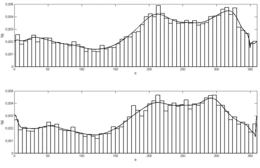
The two buoys have been chosen such that the distance between them is relatively small (33.35 nautical miles/61.77 km) and they share several features, such as similar distance to land. The data have been cleaned to erase any missing values and after this, the data set contained 24807 observations. Figure 1 shows circular Bernstein polynomial fits of the marginal densities of the wind directions at the two buoys. It can be seen that, as we might expect, the distribution of wind directions at the two sites are very similar.
As a first step, we tested the hypothesis that the two variables were independent using the approach of Alvo (1998). This test rejected the hypothesis of independence at anα= 0.01 level, which implies that it makes sense to consider using our approach to estimate the joint density of the two variables.
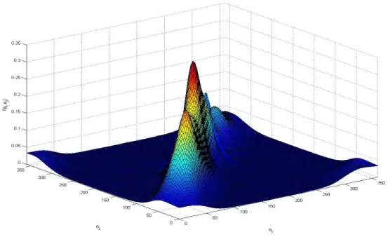
Figure 2 shows the estimated density of the circular-circular model. For better visualization, we have moved the origins of the Bernstein polynomials to the center of the graph. As we can observe, there is a high correlation between the two variables and we may assume that wind regime distributions at both buoys are very similar.
Figure 1: Marginal densities of the wind directions at the two buoys, Θ1 (top) and Θ2(bottom).
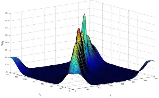
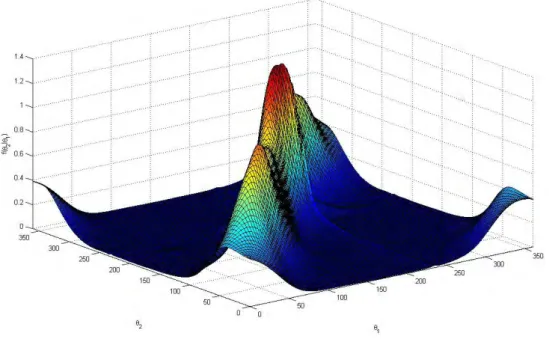
To illustrate this feature, we have computed the conditional densities for both buoys. Figure 3 shows the conditional distribution of Θ1|Θ2 and Figure 4 shows the conditional distribution of Θ2|Θ1. As can be
seen in both graphs, we have the same density along the main diagonal of the graph. This indicates the behavior of one of the buoys as a function of the other. The distributions are useful from a operational point of view, suppose that two ships departing from the nearest ports to each of the buoys and one of them is temporarily disabled for maintenance. Observing the conditional probability we can assign a route in which the fuel consumption of both boats can be optimized.
To summarize this example, we have modeled the wind direction in two nearby buoys showing the high correlated wind flow between these two sites under the lack of distorting elements such as mountains, etc. Observe that this correlation could be viewed as spatial correlation.
6.2
Circular-linear data: wind directions and rainfall
Many variables can influence the climate at a certain site, but from a meteorology (climatology or environ-mental) point of view, most studies focus on wind direction and related variables such as rainfall.
Figure 2: Estimated density function for the circular-circular model,f(θ1, θ2).
from 6/11/94 to 31/1/2009 at the observatory site at Som´ıo, near Gijon in northern Spain, at latitude 43◦32’17”N, longitude: 5◦37’26”W and 30 metres above sea level. The wind direction is measured in degrees from 0 to 359 and rainfall is measured on a grid of 0.2 liters per square meter. These data are available from
http://infomet.am.ub.es/clima/gijon/.
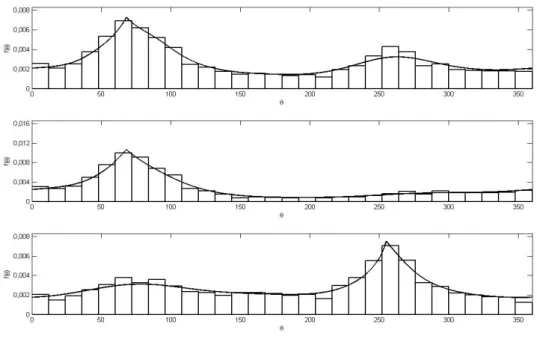
At the site, rain was recorded on about 49.2% of the days. Figure 5 shows histograms and circular Bernstein polynomial fits of the marginal density of the wind direction for the whole data set and conditioning on the weather being dry or rainy.It can be seen that there is some difference between the estimated density fits. This may be explained by the fact that sea winds are often associated with rainfall, whereas winds coming from the land to the sea, are more regularly associated with dry weather in Spain. This suggests that it is sensible to model the joint density of the wind direction, Θ, and the level of rainfall, X, by conditioning as:
f(θ, x) =f(θ|X= 0)P(X = 0) +f(θ, x|X >0)P(X >0).
Then, we can estimate ˆP(X > 0) = 0.492, ˆP(X = 0) = 0.508 and use a circular Bernstein polynomial, ˆ
fνˆ
k(θ|X= 0) to estimate the density of Θ given that there is no rain, as in the middle diagram of Figure 5.
Figure 3: Conditional density function,f(θ1|θ2)
Θ conditional on there being rain. In particular, we use the circular Bernstein copula density outlined in Section 2 to estimate the marginal density of Θ, as in the bottom diagram of Figure 5 and then apply a cubic spline smoothed density estimate of the marginal density of the level of rainfall and finally use the circular-linear copula outlined here to estimate the joint density.
Similar to the first illustration, we first carried out the hypothesis test for independence between the two variables proposed in Alvo (1998). This was rejected at an α= 0.01% level, which suggests that there is dependence between the two sets of data.
In this case we have used a Bernstein polynomial of degree 51, with origin 255oapproximately. We have constructed the figures with this origin represented as 0 and we increase the index clockwise.
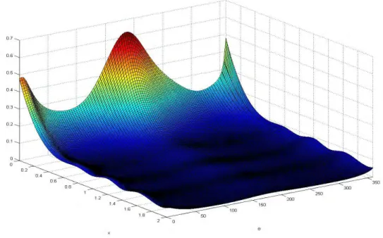
Figure 6 shows the estimated joint density, where for better visualization we only illustrate the density for rainfall levels of up to 2mm. We have used cubic splines to interpolate the values of the function where there are not data (remember that the data analyzed in this example are discretized over a grid of 0.2) to obtain a smooth function. As we can observe in the figure there are two modes corresponding to East and West approximately. As we commented earlier, the orography of this part of Spain (the Cantabrian Mountains) implies that surface winds head East or West, when orographic rain is produced.
Figure 4: Conditional density function,f(θ2|θ1)
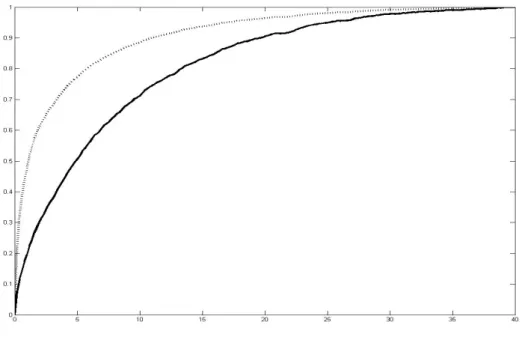
Figure 7 shows conditional distribution functions of the level of rainfall given that wind directions equal to the two modes of the previous figure. The solid line corresponds approximately to the East, which corresponds to the origin (0o), and the dotted line corresponds approximately to the West (195o). As we
can see in the figure the behavior is different due to that the cold fronts which produces intense rains termed frontal rains comes from West to East.
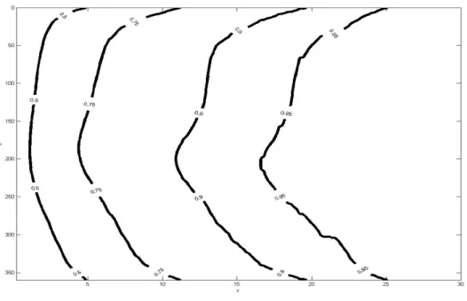
For a better visualization of this effect, Figure 8 shows a contour plot of the conditional distribution of the rainfall level given the wind direction. We show the lines corresponding to the 0.5, 0.75, 0.90 and 0.95 percentiles. Observing the graph, when the wind direction is East (0o) there is more probability of heavy rain than when the wind comes from other directions.
To summarize this example, rainy days are very influenced by the orography of this part of Spain. Two types of rain predominate, that is firstly, orographic rain which happens when humid winds encounter a mountain range and producing small quantities of rain and secondly, cyclonic or frontal rains induced by low pressure systems which come from West to East and are associated with heavy rain. As we can observe in Figure 7, the conditional rainfall level distribution for the East direction has a heavy tail.
Figure 5: Marginal densities of wind direction: whole data set (top), dry days (middle), rainy days (bottom).
7
Conclusions and extensions
In this paper, we have illustrated how to use a nonparametric approach to construct a bivariate distribution with at least a component of circular type as an alternative to the usual, parametric models for these types of data. We have applied the empirical Bernstein copula as described in Sancetta et al (2004) and introduced appropriate corrections to guarantee that the constructed bivariate distribution is strictly continuous. Our approach has been illustrated with real data examples based on wind direction and rainfall data.
Various extensions of our approach are possible.
Firstly, the selection of the values of k= (k1, k2) is an open problem. Here, we have chosen the
recom-mendation of Sancetta and Satchell (2004) which provides a relatively smooth fit, but it would be interesting to explore further possibilities. Secondly, it would be interesting to consider alternative approaches to non-parametric copula estimation. One procedure would be to use multidimensional, non-negative Fourier series as an approximating function.
Finally, it would be interesting to explore the possibility of using time varying copulas so that our approach could be incorporated in time series models for estimating wind directions. Also, it would be interesting to look at multivariate copulas so that other climatic variables could also be included.
Figure 6: Fitted bivariate density function,f(x, θ|X >0)
References
[1] Bai, Z.D., Rao, C.R., and Zhao, L.C., (1988) Kernel estimators of density function of directional data,
Journal of Multivariate Analysis, 27, 24–39.
[2] Batschelet, E., (1981).Circular Statistics in Biology, Academic Press, London.
[3] Bouezmarni, T., Rombouts, J. and Taamouti, A. (2010) Asymptotic Properties of the Bernstein Density Copula for Dependent Data,Journal of Multivariate Analysis, 101, 1–10.
[4] Carnicero, J.A., Wiper, M.P., and Aus´ın, M.C., (2010). Circular Bernstein polynomial distributions.
UC3M Working papers. Statistics and Econometrics, 10-25-11.
[5] Fern´andez-Dur´an, J.J., (2004). Circular distributions based on nonnegative trigonometric sums. Bio-metrics,60, 499–503.
[6] Fern´andez-Dur´an, J.J., (2007). Models for circular-linear and circular-circular data constructed from circular distributions based on nonnegative trigonometric sums.Biometrics,63, 579–585.
Figure 7: Conditional distribution functions,F(x|θ, X >0), given the two modal wind directions:East (solid line) and West (dotted line).
[8] Gould, A.L.,, (1969). A regression technique for angular data,Biometrics, 25, 683–700.
[9] Jammalamadaka, S.R., and Sarma, Y.R., (1988). A correlation coefficient for angular variables, in
Statistical Theory and Data Analysis II, Matusita, K., ed., North Holland, Amsterdam, pp. 349–364.
[10] Jammalamadaka, S.R., and Sarma, Y.R., (1993). Circular regression, inStatistical Sciences and Data Analysis, Matusita, K., edi., VSP, Utrecht, pp. 109–128.
[11] Johnson, R.A., and Wehrly, T.E., (1977). Measures and models for angular correlation and angular-linear correlation,Journal Royal Statistic Society, 39, 222–229.
[12] Johnson, R.A., and Wehrly, T.E., (1978). Some angular-linear distributions and related regression mod-els,Journal of American Statistic Association, 73, 602–606.
[13] Kagan, A.M., Linnik, Y.V., and Rao, C.R., (1973). Characterization Problems in Mathematical Statis-tics, John Wiley, New York.
Figure 8: Contour plot ofF(X ≤x|θ, X >0)
[15] Mardia, K.V., (1975). Statistics of directional data,Journal Royal Statistic Society, Series B, 37, 349– 393.
[16] Mardia, K.V., (1976). Linear-circular correlation coefficients and rhythmometry,Biometrika, 63, 403– 405.
[17] Mardia, K.V., and Jupp, P.E., (1999).Directional Statistics, Wiley, Chichester.
[18] Mardia, K.V., and Sutton, T.W., (1975). On the modes of a mixture of two von Mises distributions,
Biometrika, 62, 699–701,.
[19] Mardia, K.V., and Sutton, T.W., (1978). A model for cylindrical variables with applications,Journal of the Royal Statistic Society, Series B, 40, 229-233.
[20] Nelsen, R.B., (1999).An Introduction to Copulas. Springer, Berlin.
[21] Pfeifer. D., Straßburger, D., and Philipps, J., (2009) Modelling and simulation of dependence structures, inNonlife Insurance with Bernstein Copulas. The 39th International ASTIN Colloquium, Helsinki.
[22] Rives, L.P., (1982). Some statistical methods for bivariate circular data,Journal of the Royal Statistical Society, 44, 81–90.
[23] Sancetta, A., and Satchell, S.E., (2004) The Bernstein copula and its applications to modelling and approximations of multivariate distributions,Econometric Theory, 20, 535-562.
[24] Sklar, A., (1959) Fonctions de r´epartition `a n dimensions et leurs marges, Publications de l’Institut de Statistique de L’Universit´e de Paris 8, 229-231.
[25] Sklar, A., (1973) Random variables, joint distribution functions, and copulas.Kybernetika, 9, 449–460.
[26] Stephens, M.A., (1979). Vector correlation,Biometrika, 66, 41–48.
[27] Vitale, R.A., (1975) A Bernstein polynomial approach to density estimation, inStatistical Inference and Related Topics, Madan Lal Puri ed., Academic Press, New York, pp. 87–100.