RAPHAEL TARI SAMUEL
NONLINEAR DYNAMIC PROCESS MONITORING
USING KERNEL METHODS
OIL AND GAS ENGINEERING CENTRE
SCHOOL OF WATER, ENERGY AND ENVIRONMENT (SWEE)
PhD
Academic Year 2015-2016
Supervisors:
Dr Yi Cao
Dr Giorgos Kopanos
OIL AND GAS ENGINEERING CENTRE
SCHOOL OF WATER, ENERGY AND ENVIRONMENT (SWEE)
PhD Thesis
Academic Year 2015-2016
RAPHAEL TARI SAMUEL
NONLINEAR DYNAMIC PROCESS MONITORING
USING KERNEL METHODS
Supervisors:
Dr Yi Cao
Dr Giorgos Kopanos
August 2016
This thesis is submitted in partial fulfilment of the requirement for the degree of Doctor of Philosophy
c
Cranfield University, 2016. All rights reserved. No part of this publication may be reproduced without the written permission of the copyright holder.
Abstract
The application of kernel methods in process monitoring is well established. How-ever, there is need to extend existing techniques using novel implementation strate-gies in order to improve process monitoring performance. For example, process monitoring using kernel principal component analysis (KPCA) have been reported. Nevertheless, the effect of combining kernel density estimation (KDE)-based control limits with KPCA for nonlinear process monitoring has not been adequately investi-gated and documented. Therefore, process monitoring using KPCA and KDE-based control limits is carried out in this work. A new KPCA-KDE fault identification technique is also proposed.
Furthermore, most process systems are complex and data collected from them have more than one characteristic. Therefore, three techniques are developed in this work to capture more than one process behaviour. These include the linear latent variable-CVA (LLV-CVA), kernel CVA using QR decomposition (KCVA-QRD) and kernel latent variable-CVA (KLV-CVA).
LLV-CVA captures both linear and dynamic relations in the process variables. On the other hand, KCVA-QRD and KLV-CVA account for both nonlinearity and pro-cess dynamics. The CVA with kernel density estimation (CVA-KDE) technique reported does not address the nonlinear problem directly while the regular kernel CVA approach require regularisation of the constructed kernel data to avoid com-putational instability. However, this compromises process monitoring performance.
The results of the work showed that KPCA-KDE is more robust and detected faults higher and earlier than the KPCA technique based on Gaussian assumption of pro-cess data. The nonlinear dynamic methods proposed also performed better than the afore-mentioned existing techniques without employing the ridge-type regulari-sation.
Acknowledgements
The PhD route could be long and tortuous. It would not have been possible to get to this point without the support of several good spirited people. I therefore use this opportunity to express my profound gratitude to some of them.
I thank my supervisors, Dr Yi Cao and Dr Giorgos Kopanos. The professionalism exhibited by Dr Cao and his attention to details contributed immensely to the completion of this work. I thank him so dearly. Although, my contact hours with Dr Kopanos were few because he joined the supervisory team late in my research, yet his suggestions on the soft issues were very helpful.
I will also like to specially thank Sam Skears and Samara Ahmad for their assistance in administrative and immigration issues respectively. I am also grateful to my office mates, friends and colleagues: Richard, Nonso, Reward and Cristobal for making my stay at Cranfield memorable. I will not also forget to thank Rev. Olabiyi Ajala, Dr. Sola Adesola, Dr Crispin Allison and the Holding Forth/CPA family for their support during my stay at Cranfield.
I also wish to express my heart-felt gratitude to my wife, Tariere, my children, Kuro and Mercy, and my extended family for their sacrifice throughout my research work. Above all, thanks be to the Almighty God for His love and tender mercies. I dedicate this work to His Name and glory.
Contents
Contents iv
List of figures ix
List of tables xii
1 Introduction 1
1.1 Process monitoring tasks . . . 3
1.2 Motivation of the research . . . 4
1.3 Research gaps . . . 6
1.4 Aim and objectives . . . 7
1.5 Publications . . . 8
1.6 Thesis outline . . . 9
2 Overview of Process Monitoring Methods and Positive Definite Kernels 13 2.1 Model-based methods . . . 14
2.1.2 Observers . . . 15 2.1.3 Parity relations . . . 16 2.1.4 Parameter estimation . . . 16 2.2 Knowledge-based methods . . . 17 2.2.1 Causal analysis . . . 18 2.2.2 Expert systems . . . 18 2.3 Data-based methods . . . 19
2.3.1 Principal component analysis . . . 21
2.3.2 Canonical correlation analysis . . . 24
2.3.3 Dynamic Principal component analysis . . . 26
2.3.4 Canonical variate analysis . . . 28
2.4 Positive definite kernels . . . 29
2.4.1 Positive semi-definite and positive definiteness . . . 31
2.4.2 Hilbert spaces . . . 31
2.4.3 Reproducing kernels . . . 33
2.4.4 Reproducing kernel Hilbert spaces . . . 35
2.4.5 Mercer’s Theorem . . . 36
2.4.6 Feature maps associated with kernels . . . 37
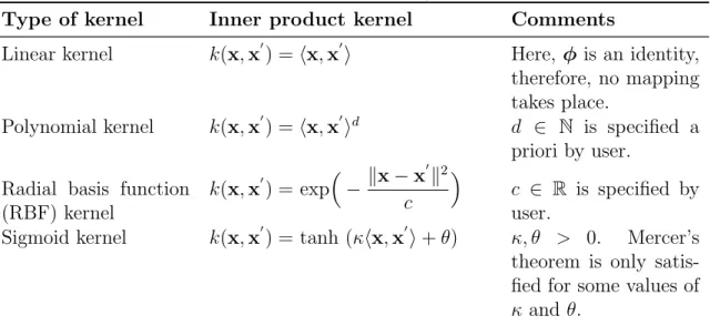
2.4.7 Examples and properties of kernels . . . 40
2.4.8 Kernel principal component analysis . . . 41
2.4.10 Nonlinear dynamic process monitoring . . . 44
2.4.11 Concluding remarks . . . 46
3 Nonlinear process fault detection and identification using kernel PCA and KDE 48 3.1 KPCA-KDE-based process monitoring . . . 49
3.1.1 Kernel PCA algorithm . . . 49
3.1.2 Fault detection metrics . . . 51
3.1.3 Kernel density estimation . . . 52
3.1.4 On-line monitoring . . . 52
3.1.5 Outline of KPCA-KDE fault detection procedure . . . 53
3.2 KPCA-KDE based fault identification . . . 54
3.3 Application study . . . 57
3.3.1 Overview of Tennessee Eastman process . . . 57
3.3.2 Application procedure . . . 58
3.3.3 Fault detection rule . . . 60
3.3.4 Computation of monitoring performance metrics . . . 61
3.3.5 Results and discussion . . . 62
3.4 Concluding remarks . . . 65
4 Statistical process monitoring using linear latent variable CVA 70 4.1 Introduction . . . 70
4.3 Method of fault detection . . . 73
4.3.1 LLV-CVA-based process monitoring steps . . . 74
4.4 Application study . . . 75
4.4.1 Parameters selection . . . 75
4.4.2 Results and discussion . . . 78
4.5 Concluding remarks . . . 80
5 Kernel canonical variate analysis using QR decomposition 83 5.1 Introduction . . . 83
5.2 QR decomposition . . . 84
5.3 Kernel CVA with QR decomposition . . . 85
5.4 Fault detection using KCVA-QRD . . . 87
5.5 Summary of KCVA-QRD-based fault detection procedure . . . 88
5.6 Application study . . . 89
5.6.1 Results and discussion . . . 90
5.7 Concluding remarks . . . 92
6 Kernel latent variable CVA for nonlinear dynamic process moni-toring 94 6.1 Introduction . . . 95
6.2 Kernel latent variable CVA . . . 97
6.3 KLV-CVA-based fault detection . . . 100
6.4 Application study . . . 101
6.4.1 Implementation details . . . 101
6.4.2 Parameter selection . . . 102
6.4.3 Results and discussion . . . 102
6.5 Concluding remarks . . . 104
7 Conclusions and further work 106 7.1 Summary and research aim . . . 106
7.2 Conclusions . . . 107
7.3 Contributions of the study . . . 108
7.4 Limitations of the Research . . . 109
7.5 Further work . . . 109
List of Figures
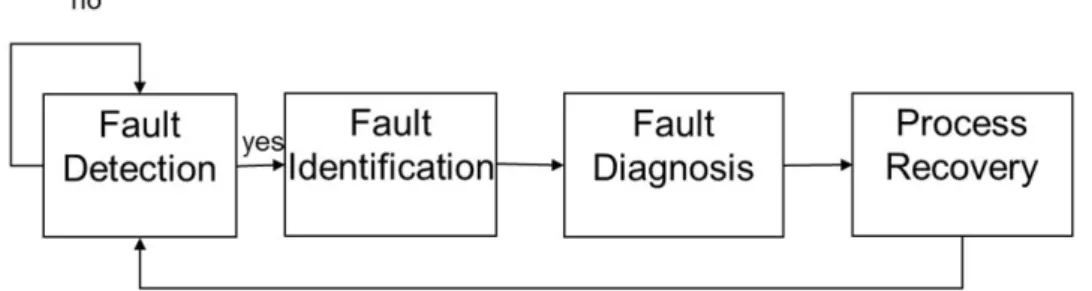
1.1 Flowchart showing four general process monitoring tasks. When fault is detected, the variables associated with fault are first identified and the process is recovered after determining the source of the fault (fault diagnosis) and removing it. . . 3
2.1 Flowchart showing the stages of a model-based fault detection and diagnosis procedure. Residuals are generated from the difference be-tween system and model outputs. The residuals are then evaluated using specified rules for a decision to made whether or not a fault has occurred. . . 14
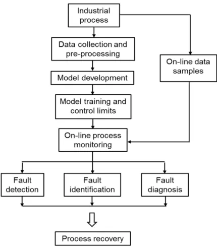
2.2 Flowchart showing a typical MSPM procedure. Normal operating data are collected and pre-processed (e.g. normalised to zero mean and unit variance). The monitoring model is developed and trained, and control limits are computed for on-line monitoring. A faulty process is recovered after successful fault detection, identification and diagnosis. . . 20
2.3 An illustration of the effect of mapping data into a high dimensional feature space. The nonlinear function φ embeds data in the feature space. Data points which were not linearly separable in the input space (left panel) become linearly separable after mapping into higher dimensions (right panel). . . 39
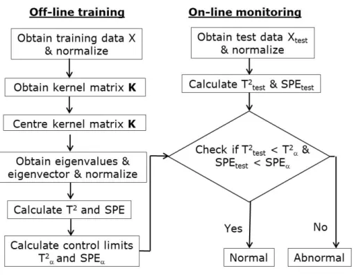
3.1 KPCA-KDE fault detection procedure. . . 54
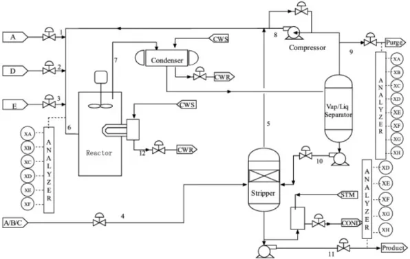
3.2 Schematic diagram of the TE process. Reaction products (Stream 7) are cooled in the condenser and sent to the separator where the vapour phase is cooled, partially purged (Stream 9) and recycled. Stream 4 strips unreacted reactants from Stream 10 and feeds them to the recycle stream while the products are collected from the exit. . 57
3.3 KPCA-based control charts showing monitoring indices and Gaussian assumption/KDE-based control limits for (a) Fault 11 (b) Fault 12. The KDE-based control limits are below the Gaussian assumption-based thresholds in both faults and give higher fault detection rates. . 67
3.4 Plot showing KPCA-KDE-based contributions to T2 and SPE for
Fault 11 of the TE process at sample number 300; (a) T2-based
con-tribution plot (b) SPE-based concon-tribution plot. Both plots correctly identified variables 9 and 32 mostly responsible for the faulty condition. 68
3.5 KPCA-KDE control charts for Fault 14 of the TE process; (a) control chart using W = 40 in the formulac=W nσ2 (b) control chart using
W = 10 in the formula c = W nσ2. The KPCA-KDE FARs do not change drastically with changing operating parameters which makes it more robust than the KPCA approach based on Gaussian assumption control limits. . . 69
4.1 Plot showing sample autocorrelation function of the training data with 95% confidence level. Autocorrelation died out at the 15th time period. Hence the length of futuref and pastg time lag was fixed at 15. . . 77
4.2 Plot of normalised singular values of the training data used for deter-mining number of states to retain. Since the singular values decreased very slowly, 26 states were retained to minimise false alarms. . . 77
4.3 Control charts for Fault 9 (a) DPCA (b) CVA (c) LLV-CVA. . . 82
5.1 Monitoring statistics of Fault 15. (a) KCVA with QRD, (b) KCVA with regularisation (10−2), (c) KCVA with regularisation (10−8). . . . 92
6.1 Flowchart showing the regular kernelisation process. In general, it involves constructing a kernel matrix using a kernel function and per-forming the required algorithm directly on the kernel matrix. . . 95
6.2 Flowchart showing an alternate kernelisation approach. It is essen-tially carrying out KPCA followed by performing any other specified algorithm on the kernel latent variables . . . 96
6.3 Monitoring statistics for Fault 3 using KLV-CVA and KCVA-REG using 2 regularisation sizes (a) CVA-KDE, (b) KLV-CVA, (c) 10−2 regularisation, (d) 10−8 regularisation . . . 105
List of Tables
2.1 Examples of commonly used kernels . . . 40
3.1 Off-line training . . . 53
3.2 On-line monitoring . . . 54
3.3 TE process monitoring variables. . . 59
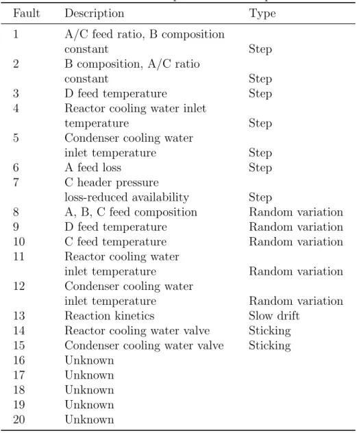
3.4 Fault descriptions in the TE process. . . 60
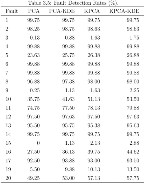
3.5 Fault Detection Rates (%). . . 63
3.6 Detection Delay, DD (min). . . 64
3.7 Monitoring results at different number of PCs retained. . . 65
4.1 Table showing summary of design parameters for the different moni-toring methods. . . 78
4.2 Table comparing FDRs of DPCA, CVA and LLV-CVA for Faults 1 to 20 of the TE process. LLV-CVA outperformed the DPCA and give FDRs comparable with the CVA. Note: All techniques gave zero false alarms. . . 80
4.3 Table comparing fault detection times (min) of DPCA, CVA and LLV-CVA for Faults 1 to 20 of the TE process. LLV-CVA performs better than the DPCA. However, detection times of the LLV-CVA and CVA are not significantly different. . . 81
5.1 Comparison of monitoring results (DKPCA, QRD and KCVA-REG). The DKPCA results are very poor in all faults while the perfor-mance of KCVA-REG depends on the regularisation parameter value. The proposed KCVA-QRD is generally better without regularisation. 91
6.1 Summary of design parameters . . . 102
6.2 Comparison of FDR and FAR. KLV-CVA performs better than CVA-KDE. KCVA-REG values depend on regularisation value used and compares with KLV-CVA values only at high regularisation. . . 103
6.3 Comparison of fault detection delay. KLV-KCVA detected faults ear-lier than CVA-KDE. KCVA-REG values depend on regularisation parameter used. . . 104
Chapter 1
Introduction
The subject of the research work reported in this thesis is the development and testing of kernel-based multivariate statistical algorithms for monitoring nonlinear dynamic processes. This introduction chapter provides the background to the work and at-tempts to address how the work fits into the broader context of the process monitoring and control discipline.
As a result of technological development, modern process facilities have become larger, more complex and highly integrated. At the same time, the regulations that govern their operations are now more stringent. Therefore, the need to operate these facilities in an efficient but sustainable manner has become more challenging and critical.
Although process controllers are able to compensate for a number of disturbances that occur in a process, there are some process changes or faults which controllers cannot handle adequately (Russel et al., 2000). These include faulty actuators or analysers, contaminated sensors, leaks, clogged filters, changing feedstock properties, degraded catalysts, etc. If they are not detected and corrected in time, these faults can cause equipment malfunction or failure, unscheduled plant or unit shut-downs, poor product quality, industrial accidents, devastating environmental impacts and huge financial losses.
In large complex industrial plants with automatic data acquisition facilities, several variables are measured and data are recorded very frequently. Therefore, the total amount of data collected during routine plant operations have increased dramati-cally. The sheer volume of data makes it difficult for human operators to react to faults appropriately. Thus, the benefits gained from closer process management due to increased data availability can often be offset by losses arising from time spent in dealing with unexpected situations. Furthermore, the large volume of data or in-formation generated from the plethora of process measurements has also increased the pressure on human operators to make very important and complex decisions often within a very short interval of time. However, information overload can make human operators prone to making decisions and taking actions that make things even worse in their attempt to correct faults. Incidents like Three Mile Island, Bhopal, and Chernobyl (Lees, 2005) are tragic examples of faults that turned into disasters, partly due to wrong actions on the part of operators, who were probably overwhelmed by too much information. Hence, the development of effective pro-cess monitoring techniques that enable automated fault detection and diagnosis in industrial systems is desirable.
Proper process monitoring will ensure timely detection of abnormal situations and give room for early intervention. This will improve safety, product quality, safeguard the environment and enhance overall system reliability. Prevention of equipment malfunctions or failures and associated cost and downtime will improve economic savings significantly and increase profitability. These incentives have spurred the study and development of automatic process monitoring methods starting from the early 1970s (Isermann and Ball´e, 1997). Furthermore, research in data-driven pro-cess monitoring methods have received much attention in the last 25 years resulting in the development of several multivariate statistical methods (Saxen et al., 2013; MacGregor and Cinar, 2012; Yin et al., 2014; Ding et al., 2013; Dai and Gao, 2013).
1.1
Process monitoring tasks
Process monitoring is the checking of measurable variables against tolerances and raising alarms for operator action when a tolerance is exceeded (Isermann, 2005). The goal of process monitoring is to detect, identify and diagnose faults timely so that appropriate actions are taken to remove assignable cause(s) while the process is still controllable. Consequently, process monitoring is associated with the following tasks (Raich and Cinar, 1996): fault detection, fault identification, fault diagnosis and process recovery or intervention (Fig. 1.1).
Figure 1.1: Flowchart showing four general process monitoring tasks. When fault is detected, the variables associated with fault are first identified and the process is recovered after determining the source of the fault (fault diagnosis) and removing it.
• Fault detection: determining the occurrence of a fault.
• Fault identification: identifying the variables immediately impacted by a fault.
• Fault diagnosis: determining the source of the fault.
• Process recovery or intervention: removing the effect of the fault.
It is necessary to note here, that the terminology associated with process moni-toring lacks consistency in the fault detection and diagnosis (FDD) literature. For instance, Isermann and Ball´e (1997) defines fault diagnosis as the determination of the nature, time, locality and extent of a given fault. An alternative viewpoint is that fault diagnosis consists of fault isolation and fault identification (see Gonzalez
and Castanon, 2011, pg. 99). According to this viewpoint, fault isolation is the de-termination of the faulty component while fault identification is the dede-termination of the magnitude of the fault. In this context, the term fault detection and isolation (FDI) is adopted when the identification task is not deemed to justify the effort. In some cases, “diagnosis” is used only as a synonym to “isolation” (Gertler, 1998, pg. 3).
1.2
Motivation of the research
Techniques based on multivariate statistics are well suited for monitoring large com-plex processes. These approaches which are generally referred to as multivariate statistical process monitoring (MSPM) methods or statistical process control (SPC) can be used to process multidimensional data and account for correlation or redun-dant information in data. MSPM approaches are more effective and more efficient than univariate methods. Univariate methods deal with only one variable at a time. Therefore, they lack the ability to describe relationships between variables in a dataset. Furthermore, multivariate statistical techniques can be used to perform dimensionality reduction. Hundreds or even thousands of highly correlated variables can be reduced to a few latent variables without sacrificing critical information. The lower dimensional data can be further reduced to three, two or even one monitoring measure(s). This simplifies the monitoring process and improves working conditions by helping operators to focus on fewer variables to monitor.
Nevertheless, traditional MSPM techniques such as principal component analysis (PCA) (Wold et al., 1987; Jolliffe, 2002) and partial least squares (PLS) (Wilson and Irwin, 2000; Muradore and Fiorini, 2012) assume that the process being monitored is linear and static. On the contrary, nonlinearity and dynamics exist widely in the process industry. Therefore, traditional MSPM techniques perform poorly in practice (Yin et al., 2012). Hence, there is need to develop process monitoring algorithms that effectively capture process nonlinearity and dynamics in order to improve monitoring performance (Chen, 2013; Yang et al., 2012). This need serves
as part of the motivation for this research work.
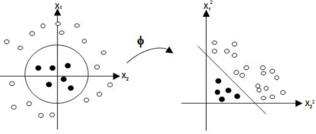
To address the nonlinearity problem, traditional techniques such polynomials, splines, and neural networks (NNs) have been used (Mathews, 1991; Wold, 1992; Kramer, 1992; Haykin, 1999). However, many of these approaches involve iterative nonlinear solution methods and/or are computationally expensive. In particular, NNs suffer from long-time training, slow convergence and local minima (Gou and Fyfe, 2004). More recently, kernel methods, have gained popularity as an attractive framework for tackling nonlinear problems (Sch¨olkopf and Smola, 2002; Shawe-Taylor and Cris-tianini, 2004). The key principle of kernel methods which is also the main motivation for using kernel methods in this work is thekernel trick.
The kernel trick is based on the fact that many data processing approaches depend on the inner products between data samples; not on the individual data samples. It is therefore possible to develop a nonlinear extension of a linear algorithm by mapping the original data into a high-dimensional feature space via a nonlinear mapping and reformulating the algorithm in a way that needs only values of the inner products in the feature space. In kernel methods, the inner products of the mapped samples in the high dimensional feature space are defined by using a kernel function of the corresponding samples in the original data space (Qin, 2012; Honeine and Richard, 2011a). Hence, kernel algorithms are very efficient and do not involve high computational complexity.
Valid kernels can be constructed for even non vectorial data such as strings and graphs by simply replacing the classical inner product by an appropriate similarity measure for the data. Therefore, kernel methods have extended the use of classi-cal algorithms to many situations where data cannot be readily represented in a vectorial form by directly working with pairwise distances or similarities between non-vectorial objects (Duin et al., 1998).
Kernel methods were proposed by Vapnik in Support Vector Machines, SVMs (Vap-nik, 2000) but are now employed in classification (Mika, Ratsch, Weston, Sch¨olkopf and Muller, 1999), regression (Rosipal and Trejo, 2002), bioengineering
(Camps-Valls et al., 2006), and image de-noising (Mika, Sch¨olkopf, Smola, M¨uller, Scholz and R¨atsch, 1999). Successful application of kernel methods have also been re-ported in time series prediction (Richard et al., 2009), novelty detection (Sch¨olkopf et al., 1999), and process condition monitoring (Lee et al., 2004; Choi et al., 2005; Tan et al., 2010).
1.3
Research gaps
Although kernel-based process monitoring is not new, the need for extending ex-isting approaches and developing alternative implementation strategies to improve monitoring performance still exist. For example, a number of nonlinear process monitoring studies using kernel PCA (KPCA) have been reported. Nevertheless, the effect of combining kernel density estimation (KDE)-based control limits with KPCA for nonlinear process monitoring has not been adequately investigated and documented. Hence, a study on process monitoring using KPCA and KDE-based control limits is carried out in this work. In particular, the performance and ro-bustness of KPCA-KDE-based process monitoring is determined and the results obtained are compared with results obtained with KPCA and control limits based on the assumption of normally distributed process data.
Furthermore, due to the nonlinear transformation involved in kernel methods, till date, fault identification is still an unsolved problem in kernel-based nonlinear pro-cess monitoring (Deng et al., 2013). The techniques reported in the literature are computationally expensive and difficult to generalise. Consequently, a new KPCA-KDE-based fault identification process is proposed in this thesis.
More importantly, very limited research has been reported on the use of kernel methods in nonlinear dynamic process monitoring. The dynamic principal compo-nent technique proposed by Choi and Lee (2004) does not capture process dynamics adequately. Conversely, canonical variate analysis (CVA) is reported to be an ef-ficient multivariate approach for monitoring dynamic systems (Ruiz-C´arcel et al.,
2015) but it does not address nonlinearity. The CVA with KDE technique proposed by Odiowei and Cao (2010) to adapt the CVA for nonlinear dynamic process moni-toring did not address the nonlinear problem directly. On the other hand, directly applying the kernel canonical correlation analysis (KCCA) algorithm to dynamic systems result in singular kernel matrices which require regularisation in order to avoid potential computational instabilities (Huang et al., 2009; Sch¨olkopf and Smola, 2002; Giantomassi et al., 2014). Furthermore, such an approach often leads to poor process monitoring performance.
To address the above problems, two new kernel-based methods are proposed in this thesis for nonlinear dynamic process monitoring. These techniques address both nonlinearity and process dynamics directly and do not require the determination of an optimum regularisation parameter value to perform well.
1.4
Aim and objectives
The main aim of this work is to develop and test kernel-based multivariate statistical algorithms for improved nonlnear dynamic process monitoring. Specifically, the objectives of this research are to:
1. Study the effect of combining kernel density estimation (KDE)-based confi-dence limits with KPCA for nonlinear process monitoring instead of using confidence limits based on the Gaussian assumption.
2. Develop a novel kernel-based approach for fault identification in a nonlinear process.
3. Develop the linear latent variable-CVA (LLV-CVA) approach for monitoring linear dynamic processes.
4. Develop a new kernel CVA technique based on QR decomposition.
5. Develop the kernel latent variable-CVA (KLV-CVA) approach for monitoring nonlinear dynamic processes.
6. Evaluate the fault detection performance of the techniques developed.
7. Carry out comparison study of the developed approaches with existing meth-ods.
1.5
Publications
Four conference papers and one journal article have resulted from this work. A second journal paper has been submitted.
Conference papers
Samuel, R.T. and Cao, Y. (2014), Fault detection in a multivariate process based on kernel PCA and kernel density estimation, 20thInternational Conference on
Automa-tion and Computing (ICAC) Cranfield, Bedfordshire, United Kingdom, September 12-13, pp. 146-151.
Samuel, R. T. and Cao, Y. (2015), Kernel canonical variate analysis for nonlinear dynamic process monitoring, 9th International Symposium on Advance Control of
Chemical Processes, Whistler, British Columbia, Canada, June 7-10, pp. 606-611. (This paper was awarded as the best presentation paper at the conference).
Samuel, R.T. and Cao, Y. (2015), Improved Kernel Canonical Variate Analysis for Process Monitoring, 21st International Conference on Automation and Computing
(ICAC), University of Strathclyde, Glasgow, UK, September 11-12, pp. 341-346.
Samuel, R. T. and Cao, Y. (2016), Dynamic latent variable modelling and fault detection of Tennessee Eastman challenge process, IEEE International Conference on Industrial Technology (ICIT), Taipei, Taiwan, March 14-17.
Journal articles
Samuel, R. T. and Cao, Y. (2016), Nonlinear process fault detection and identifica-tion using kernel PCA and kernel density estimaidentifica-tion, Systems Science and Control Engineering, 4(1), 165-174.
Samuel, R. T. and Cao, Y., Kernel latent variable CVA for nonlinear dynamic pro-cess monitoring, IEEE International Transaction on Industrial Informatics - Sub-mitted.
1.6
Thesis outline
This thesis consists of seven chapters. The first two chapters are introduction and an overview of process monitoring methods respectively. Chapters 3 to 6 contain in-dividual algorithms developed in this thesis. These chapters employ the kernel prin-ciple except Chapter 4 which is a linear dynamic method. All of the four chapters are presented in a journal publication style commonly used in the process monitor-ing literature - introduction, methodology and application study. The application study section covers algorithm testing, results/discussion and concluding remarks. Chapter 7 summarises the conclusions drawn from the work and highlights recom-mendations for future work. A summary of each of the seven chapters is presented below.
Chapter 1: Introduction
In Chapter 1 the background and motivation of the thesis is presented. The gap this research work seeks to address, the aims and objectives of the work are also presented in this chapter. The chapter ends with a thesis outline.
Chapter 2: Overview of process monitoring methods
Chapter 2 gives an overview of process monitoring methods. Some basic definitions and the theory of kernel functions is also presented in this chapter.
Chapter 3: Nonlinear process fault detection and identification using kernel PCA and kernel density estimation
In Chapter 3, the kernel KPCA with KDE technique is developed and evaluated. Fault detection and identification performance as well as robustness of the technique are assessed and compared with KPCA based on the Gaussian assumption.
Chapter 4: Statistical process monitoring using linear latent variable CVA
It is possible for a process to posses both linear and dynamic properties. A technique capable of capturing both of these properties is therefore necessary. In this chapter, the linear latent variable technique (LLV-CVA) is developed to address this case. The effectiveness of the techniques is assessed and compared with the DPCA and CVA using the TE process.
Chapter 5: Kernel canonical variate analysis using QR decomposition
Chapter 5 is dedicated to the development of the kernel CVA technique based on QR decomposition. The approach is also tested on the Tennessee Eastman process and the results are presented.
Chapter 6: Kernel latent variable CVA for nonlinear dynamic process monitoring
Chapter 6 addressed the development of kernel latent variable CVA (KLV-CVA) for monitoring nonlinear dynamic processes. The technique is tested on the three difficult faults (3, 9 and 15) of the TE process. The performance of the technique is compared with the traditional KCVA based on KCCA and the kernel dynamic PCA (KDPCA).
Chapter 7: Conclusions and future work
This chapter summarizes how the objectives of the research were fulfilled. The contributions and limitations of this work are also presented in this chapter. The chapter ends with some recommendations for future work.
Chapter 2
Overview of Process Monitoring
Methods and Positive Definite
Kernels
An overview of process monitoring methods is presented in this chapter. The chap-ter also provides some relevant definitions and the theory of kernel functions - the key ingredient of kernel methods. The concept of reproducing kernel Hilbert spaces, nonlinear mapping and the feature space, and the general implementation strategy implied in kernel methods are discussed. Common examples of kernels and kernel-based algorithms are also presented.
Process monitoring methods may be classified into three categories: data-based, knowledge-based and model-based (Chiang et al., 2001). An elaborate discussion and description of these categories is captured in a three-part series by Venkata-subramanian and other researchers published in 2003. The different monitoring categories are reviewed in this section.
2.1
Model-based methods
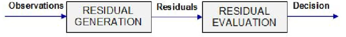
Model-based or analytical approaches are based on explicit mathematical models of the monitored plant (Isermann, 1984). These fundamental models describe the internal dynamics and explain the behaviour of the process based on physical, chem-ical or biologchem-ical laws. Most model-based fault detection and diagnosis methods are based on the concept of analytical redundancy. This involves comparing measured performance or outputs with analytically predicted or estimated outputs. It can also mean comparing values of two analytically computed quantities from different sets of variables. This is in contrast to physical redundancy which involves comparing measurements obtained from several sensors. In analytical redundancy methods, the occurrence of a fault is captured by the difference between the plant output and the model prediction or estimate (that is, the residual). Thus, residuals can be thought of as “artificial signals” that reflect possible faults of the process. Techniques such as parameter estimation (Isermann, 1993), observer based design (Frank, 1990) or parity relations (Xiong et al., 2006) are used to generate the residuals.
The analytical redundancy approach in model-based fault detection and diagnosis consists of two key stages: residual generation and residual evaluation (see Fig. 2.1). In the residual generation stage, the difference between the system and model out-puts is generated. On the other hand, in the residual evaluation stage, the decision rules used for analysing the residuals to arrive at the monitoring decisions are chosen. This stage is essentially the decision making stage.
Figure 2.1: Flowchart showing the stages of a model-based fault detection and diagnosis procedure. Residuals are generated from the difference between system and model outputs. The residuals are then evaluated using specified rules for a decision to made whether or not a fault has occurred.
if no fault exists. Hence, residuals are usually tested against empirically or theoreti-cally derived thresholds to detect the presence of faults. The four residual generation methods associated with model-based process monitoring listed in Chapter 1 are now presented.
2.1.1
Kalman filter
The generation of residuals by Kalman filters for fault detection and diagnosis was introduced by Mehra and Peschon (1971). This technique is a recursive data pro-cessing algorithm that uses series of measurements observed over time which contain statistical noise and inaccuracies to estimate unknown variables. The difference be-tween the process measurement and the algorithm output (prediction error) is used to monitor the process. Fault diagnosis is done by carrying out statistical tests on whiteness, mean and covariance of the residuals (Hwang et al., 2010). Statistical tests based on the Kalman filter framework are easy to construct because the resid-uals form uncorrelated time-series. Nevertheless, fault diagnosis is believed to be awkward as it requires running one filter for every suspected fault and for every possible arrival time. In addition, filter outputs need to be checked to identify the one that can be matched with the actual observations (Gertler, 1998).
2.1.2
Observers
An observer is a tool used to estimate the internal states of a system based on the measured inputs and outputs. The key concern of this method is to generate sets of residuals that detect and identify different faults in a unique way. This is achieved by designing observers which are sensitive to a different subset of faults and insensitive to other faults and the unknown inputs. Essentially, under normal operating conditions, the observer estimates will closely follow the plant output resulting in a small residual which reflects the unknown inputs only. However, when a fault occurs, observers that have been designed to be insensitive to the
subset of faults will maintain small residuals which reflect the unknown inputs only. Nonetheless, observers that are sensitive to the faults will give results that differ significantly from the process giving rise to large residuals. The unique residual patterns generated by different observers for different faults enhances the monitoring process. However, the models may involve complex computations (Chiang et al., 2001; Gertler, 1991).
2.1.3
Parity relations
This technique involves checking the parity or consistency of the mathematical equa-tions of the system with the actual measurements. A fault is declared to have oc-curred when the preassigned threshold is exceeded. The parity relations can be subjected to a linear dynamic transformation for the transformed residuals to be used for dynamic process monitoring (Gertler, 1997). The design freedom arising from the transformation can be used to enhance the monitoring process. It has been shown that once the design objectives are selected, parity equations and observer based designs lead to equivalent residual generators (Gertler, 1991).
2.1.4
Parameter estimation
This is a natural approach to monitoring parametric faults. It involves building a reference model under a fault-free condition. Then, the parameters are re-identified repeatedly and the results obtained are compared with the reference model. De-viations from the reference model (that is, the residual) is then used as the basis for fault detection and diagnosis. This approach can be adopted only if a relation between process faults and changes in the model parameters exist and if suitable mathematical models are available (Chiang et al., 2001).
Mathematical models have been used for process monitoring and diagnosis for many decades (Campos-Delgado and Espinoza-Trejo, 2011; Rothenhagen and Fuchs, 2009). Since they are based on solid physical or engineering principles and prior
process knowledge, they give the most accurate results if they are well formulated. However, they can be complex and computationally intensive. Furthermore, detail understanding of all the phenomena at play in a complex large-scale process may be lacking. Therefore, significant amount of time and money is required to establish reliable quantitative models. Sometimes it is even infeasible to build one (Ge et al., 2013).
According to Katipamula and Brambley (2005), model-based process monitoring methods are not likely to emerge as the methods of choice in the near future due to the drawbacks enumerated earlier.
2.2
Knowledge-based methods
Knowledge-based approaches adopt the use of qualitative models e.g. causal analy-sis, expert systems or pattern recognition to derive the monitoring measures (Venkata-subramanian, Rengaswamy and Kavuri, 2003). No explicit system models are re-quired for these approaches and their monitoring results are very intuitive. They are therefore used as complementary methods or as alternatives to model-based ap-proaches. However, to a large extent, knowledge-based methods depend on previous knowledge of the behaviour of the process and the expertise of experienced plant operators. Therefore, it takes considerable time and effort to acquire the needed knowledge and expertise to routinely construct knowledge-based models for large-scale complex systems. Due to their weaknesses, model-based and knowledge-based methods are limited to relatively small systems; or systems for which it is easy to build the needed process model; or system for which adequate accumulation of the pertinent process knowledge is available.
To determine process status, knowledge-based methods employ prior knowledge of the process expressed in terms of qualitative relationships. This is in contrast to model-based methods discussed earlier in which prior process knowledge is expressed in terms of quantitative mathematical relationships. Therefore, process monitoring
methods based on knowledge-bases are also called qualitative model-based methods. These models can be obtained by modelling the causal relationships that exist in the system, using expert domain knowledge, and from detailed system descriptions or fault-system relationships (Chiang et al., 2001).
2.2.1
Causal analysis
Causal analysis methods are based on modelling the causal relationship between faults and symptoms in a system. Signed directed graph (SDG) is an example of causal analysis technique used mainly for fault diagnosis.
SDG is based on analysing initial and final responses of system variables due to deviations and deducing these dynamic behaviours using causal path propagations. SDG was first proposed for modelling chemical processes by Iri et al. (1979). A documentation of a systematic framework for developing and analysing SDG-based modelling has been made by Maurya et al. (2003).
It is also possible to draw conclusions on the overall system behaviour based on an understanding of the laws that govern the various subsystems. This approach is commonly called abstraction hierarchies. Its application in the process industry is well documented in Venkatasubramanian, Rengaswamy and Kavuri (2003).
2.2.2
Expert systems
The idea behind this approach is to mimic how a human expert will reason when diagnosing a fault. This is done by combining knowledge gained from first principles (or structural description of the process) with rules formulated from the experience of a domain expert. They are basically if-then-else statements and a mechanism that searches through the rule-space to arrive at conclusions deployed as a software package. These rules can be based purely on expert domain knowledge gained from experience or from first principles. Expert systems can capture diagnostic associations identified by humans which cannot be easily expressed in the form of
mathematical or causal relationships. The use of expert systems in process industries is described in detail in Venkatasubramanian, Rengaswamy, Kavuri and Yin (2003).
Expert systems are supposedly based on transparent reasoning and clear explana-tions can be provided for inferences made (Venkatasubramanian, Rengaswamy and Kavuri, 2003). However, they are system specific and fail woefully when operated outside the incorporated boundaries. They are also not easy to change or update.
2.3
Data-based methods
Data-based methods require only input and output data collected from routine pro-cess operations. These data are transformed in several ways (a propro-cess known as feature extraction) and used as prior knowledge of the monitored system. Due to their data-driven nature, neither rigorous system models nor detail process knowl-edge is required in data-based techniques. Therefore, they are simpler to build for complex large-scale systems than the model-based or knowledge-based approaches. Furthermore, historical data collected from processes are readily available and pow-erful data mining techniques for extracting process knowledge from measurement information are well understood.
Part III of the three-part review articles by Venkatasubramanian and other re-searchers published in 2003 cited in the preceding sections is dedicated to database process monitoring methods. An in-depth outlook of data-based monitoring ap-proaches is also provided by Ge et al. (2013). Their work reviewed the natures of industrial processes, data characteristics (e.g. high dimensionality, nonlinear data relationships, non-Gaussian variable distributions, time-varying and multi-mode be-haviours and data autocorrelations) as well as methodology issues and implementa-tion procedures. Figure 2.2 shows a generalised methodology for MSPM approaches.
Collecting the dataset that correctly represent the operating conditions of the pro-cess to be monitored is an important initial step in MSPM techniques. This is
Figure 2.2: Flowchart showing a typical MSPM procedure. Normal operating data are collected and pre-processed (e.g. normalised to zero mean and unit variance). The monitoring model is developed and trained, and control limits are computed for on-line monitoring. A faulty process is recovered after successful fault detection, identification and diagnosis.
needed to avoid numerous false alarms or missed detections which are indications of an inefficient monitoring technique. Pre-processing involves transforming the origi-nal dataset to a form more appropriate for developing a reliable monitoring model. A common example of pre-processing is normalising the original data to zero means and unit variance. This is done to eliminate the influence of the different scales of the various process variables to avoid undue inclination of a given model to any one of the measured process variables. The appropriate process monitoring model is then selected based on the data characteristics of the process. The model is then trained and evaluated to ascertain its efficiency. Model training is done off-line using data collected under normal operating conditions. During the training phase,
ap-propriate statistics used for online monitoring are constructed and their thresholds or control limits are computed.
To construct the monitoring statistics, the original process variables spanning a high dimensional space are projected onto a lower dimensional space spanned by
q dominant latent variables which adequately capture the relevant information in the original high dimensional data. The q latent variables are then used to derive the model for monitoring the model space (that is, the space spanned by q latent variables). Conversely, the latent variables that are not included in the model space are regarded as noise and are used to monitor the residual space (that is, the space spanned by the latent variables not included in the model space). Hotelling’s T2
and the Q statistic (also known as squared prediction error, SPE) are two indices commonly used in MSPM approaches. The T2 is used to monitor variation in the model space while theQ statistic is used to monitor variation in the residual space. Some traditional data-driven MSPM approaches and their extensions are discussed in the following subsections.
2.3.1
Principal component analysis
Principal component analysis (PCA) is probably the most popular of the MSPM methods. Assuming a dataset withn number of observations and m variables X∈ <m×n which is mean-centred and have unit variance, the sample covariance matrix
is computed as
C= 1
m−1X
T
X, (2.1)
where the subscript, T represents transpose. The eigenvalue decomposition of C
given by
C=PLPT, (2.2)
where P are the principal directions (or loading vectors) and L is the eigenvalue matrix whose ith element represents the variation present in the data projected in
scores or linear latent variables associated with the dominantq singular values. The projections of the original variables inX into the lower dimensional space is defined as Z=XP=⇒Xˆ =ZPT = q X i=1 zipTi, (2.3)
where zi is an orthogonal score vector which captures the relationship between ob-servations. Conversely, pi is an orthonormal loading vector containing information
about relationship between variables. Given that q principal components explain the variability of the process data through X, the residual matrix E that captures the variations associated with them−q singular values is given by X−Xˆ. Hence,
X =ZPT +E=
q
X
i=1
zipTi +E. (2.4)
Since ZPT and E represent the main sources of process variability (useful infor-mation) and noise (error) respectively, the choice of q (that is, the number of PCs retained) is very important in PCA-based process monitoring. Retaining too few components gives an under-fitted model. Interpreting data analysis under such a situation implies relating only to the most dominant part of the data structure. Therefore, some significant information of the data structure will not be captured. Conversely, using too many components result in an over-fitted model which runs the risk of interpreting parts of the noise in the data. A number of methods have been suggested for determining q. These include scree tests, the average eigenvalue approach, cross-validation, parallel analysis, Akaike information criterion, and the cumulative percent eigenvalue. However, none of these methods have been proved analytically to be the best in all situations (Chiang et al., 2001).
PCA-based monitoring statistics
The Hotelling’sT2 and Q statistic or squared prediction error (SPE) are commonly
squared scores. It is computed as
T2 = [z1, . . . , zq] Λ−1[z1, . . . , zq]T , (2.5)
whereqare the number of PCs retained and Λ−1 represents the inverse of the matrix of eigenvalues corresponding to the retained PCs. The control limit corresponding to a significance level,α,Tα2 is derived from the F-distribution analytically as
Tα2 ∼ q(m−1)
m−q Fq,m−q,α, (2.6) Fq,m−q,α is the value of the F-distribution corresponding to a significance level, α,
with degrees of freedomqandm−qfor the numerator and denominator respectively.
On the other hand, the squared prediction error orQ statistic is computed as
Q=eTe= I−P PTx, (2.7)
where e is the residual vector (a projection of the observation x into the residual space) andI is the identity matrix. The upper confidence limit for the Q-statistic is computed from its approximate distribution as follows (Jackson, 1991):
Qα =θ1 " Cαh0 √ 2θ2 θ1 + 1 + θ2h0(h0−1) θ2 1 #h1 0 , (2.8) where, θi = n X j=q+1 λij,(i= 1,2,3), h0 = 1− 2θ1θ3 3θ2 2
, λi are the eigenvalues, and Cα is
the 100(1−α) normal percentile.
PCA is essentially a dimensionality reduction technique based on a single collection of variables. However, situations often arise where two sets of variables (X,Y) are considered in multivariate statistical analysis. Methods used to handle such data include but not limited to multiple linear regression (MLR), PLS and CCA. MLR has severe problems dealing with large sets of correlated data. Apart from being cumbersome, MLR may lead to imprecise parameter estimates and poor predictions.
Conceptually, PLS is similar to PCA except that it reduces the dimensions of the two set of variables simultaneously to find their latent vectors which have the highest correlation using an iterative approach. A number of the techniques employed to address the gaps identified in this thesis (LLV-CVA, KCVA-QRD and KLV-CVA) are based on the principle underlying the formulation of CCA. Therefore, a discussion on the CCA is presented in the next subsection.
2.3.2
Canonical correlation analysis
Canonical correlation analysis was first proposed by Hotelling (1936). The goal of CCA is to identify and assess linear relations existing between two multivariate data sets by finding linear combinations of the original variables which maximise the correlation between the combinations. The linear combinations are called canonical variates while the pairwise correlations are known as canonical correlations. The strength of the association between the two sets of variables is measured by the canonical correlations.
Given two random variable vectors,x∈ <pandy∈ <p, their linear combinations are
defined by,u=xTaandv =yTb, whereaandbare combination coefficient vectors.
Canonical correlation analysis seeks to findaandbsuch that the correlation between
u and v is maximised. Numerically, let X∈ <N×p and Y ∈ <N×p be N samples of
xand y, respectively. Assuming expectations, E(x) =µ1 and E(y) =µ2. Define
X= µT 1 .. . µT 1 , Y = µT 2 .. . µT 2 .
Covariance and cross-covariance matrices are defined as Σxx =E n X−X X−XTo , (2.9) Σyy =E n Y−Y Y−YTo, (2.10) Σxy =E n X−X Y−YTo. (2.11)
whereE denotes expectation. In this case, correlation is given by:
ρ = max a,b aTΣ xyb (aTΣ xxa) 1/2 (bTΣ yyb) 1/2. (2.12)
Computing the standardised coefficients (weights) directly as u = Σ1xx/2a and v =
Σ1yy/2b, the CCA optimisation problem can be formulated as max u,v u T Σ−xx1/2ΣxyΣ−yy1/2 v, (2.13) s.t. uTu=vTv= 1, (2.14)
where the solution, u and v are the left and right singular vectors of the product matrix L1 =Σxx−1/2ΣxyΣ−yy1/2. Singular value decomposition can then be performed
onL1 as shown below:
L1 =Σ−xx1/2ΣxyΣyy−1/2 =U1S1VT1 (2.15)
whereU1 and V1 are orthogonal matrices of the left and right singular vectors and
S1 is a diagonal matrix whose elements are the singular values of L1. Sorting the
elements ofS1 in descending order and reordering the columns ofU1 and V1, gives
the degree of correlation between columns ofU1 and V1.
MSPM approaches such PCA and CCA are static techniques. They are based on the assumption that the process data collected are time-independent. However, data generated from many real industrial processes exhibit time-dependence. Time-dependence means that an observation at the present time period is correlated with observations before and after the present time period (Yin et al., 2012). This
phe-nomenon is known as serial correlation, lagged correlation or autocorrelation. It is caused by system dynamics arising from process units that induce inertia (that is, tendency of a system to remain in the same state from one observation to the next), and high sampling rates used in modern data acquisition instrumentation (Rato and Reis, 2011; Vanhatalo and Kulahci, 2015).
Autocorrelation affects the number of independent observations. Therefore, the covariance matrix constructed from autocorrelated data without accounting for time lags cannot adequately represent the complete variation in the data. Hence, static techniques which are usually based on zero-lag covariance matrices give poor results when applied to autocorrelated data resulting from process dynamics (Jiang, Huang, Zhu, Fan and Braatz, 2015). Consequently, significant research efforts have been made in the past years to improve monitoring performance in dynamic industrial processes by incorporating the dynamic information of the process data into the monitoring model.
The simplest way to eliminate the effects of process dynamics is to increase the sampling time. This approach weakens the correlation between the data. However, it does not take into account the dynamic relationships that exist between the process variables. Hence, long sampling time reduces the sensitivity of monitoring systems and delay fault detection especially for faults that only cause changes in the time series correlation of the process variables. Therefore, other more effective methods for monitoring dynamic processes are presented next.
2.3.3
Dynamic Principal component analysis
Dynamic principal component analysis (DPCA) is an extension of the PCA tech-nique that accounts for serial correlations. It involves augmenting each observation vector with the previousl observations and stacking the data matrix as follows:
Xl= xT t xTt−1 . . . xTt−l xTt−1 xTt−2 . . . xTt−l−1 .. . ... . .. ... xTt+l−m xTt+l−1 . . . xTt−m , (2.16)
where Xl is the augmented data matrix and xTt is the n-dimensional observation
vector in the training data at a time periodt. To extract the autocorrelation of the process data, the DPCA model is constructed by performing PCA directly on Xl.
The value ofl can be determined statistically. However, according to Chiang et al. (2001), one or two lags are appropriate for DPCA-based process monitoring. The
T2 and Qstatistics based on the DPCA are employed in a similar way as those from
the conventional PCA for process monitoring in the model and residual spaces.
Due to their simplicity, dynamic MSPM methods are used in many cases with other developed methods. Ku et al. (1995) employed the DPCA for fault detection and isolation. Tsung (2000) examined an integrated approach to simultaneously monitor and diagnose an automatic controlled process using DPCA and minimax distance classifier. Similar to the DPCA, a dynamic version of the PLS (DPLS) was proposed by Komulainen et al. (2004) while application of DPCA and DPLS techniques in on-line monitoring of batch processes was reported by Chen and Liu (2002).
The above studies showed that dynamic MSPC methods outperformed their static counterparts. Nevertheless, it is argued dynamic MSPC methods provide only lim-ited representation of process dynamics (Li et al., 2011; Russell et al., 2000). Kruger et al. (2004) also demonstrated that auto-correlated score variables will arise, even in the abstract case where the process variables are uncorrelated and a DPCA model is established. They therefore proposed the integration of ARMA models into a MSPM model. The results of case studies indicated that their approach extracts the auto-correlation of the process data successfully and provided better process monitoring performance in large-scale processes compared to the traditional dynamic MSPM
methods. The use of decorrelated residuals (Rato and Reis, 2013) have also been proposed to improve DPCA-based process monitoring. The CVA, a subspace mod-elling approach which identifies the state space model of a process, is another method widely reported for dynamic process monitoring (Jiang, Zhu, Huang, Paulson and Braatz, 2015). The CVA approach is discussed in the next subsection.
2.3.4
Canonical variate analysis
The CVA is an application of the CCA on time series data. It accounts for autocor-relation in addition to cross-corautocor-relation between variables by considering both the past and future process outputs at each time point (Wang et al., 2010; Odiowei and Cao, 2010). Assuming thatx(k)∈ <m are m process measurements (variables) at a
given time point k acquired during normal operating process conditions. The past (p) and future (f) observation vectors are defined to capture the dynamics of the process as follows: xp(k) = x(k−1) x(k−2) .. . x(k−p) ∈ <mp and x f(k)= x(t) x(k+1) .. . x(k+f−1) ∈ <mf (2.17)
The respective past and future observation vectors are then combined separately to obtain the past and future matrices Xp and Xf. Defining ˜Xp = Xp −Xp and
˜
Xf =Xf −Xf as the centred past and future matrices, where Xp and Xf are the
sample means, the covariance and cross-covariance matrices of the past and future observations are obtained as:
Σpp=E ˜ XpX˜Tp , Σf f =E ˜ XfX˜Tf , Σf p=E ˜ XfX˜Tp (2.18)
The product matrix H1 from (2.18) is obtained and decomposed as follows: H1 =Σ −1/2 f f Σf pΣ −1/2 pp =U3S3V3T (2.19)
The linear combinations of the past observations that best explain the variability of the future observations are obtained by performing SVD on H1 in (2.19). In order
to compute the monitoring statistics, the state variables (which span the model space) and the residuals are obtained from the transformed past observations. The
T2 andQstatistics are calculated at each time point as the sum of the squared state
variables and residuals respectively. These computations are presented in chapters 4, 5 and 6.
The application of CVA in system identification was pioneered by Akaike (1975) and was adapted to general linear systems by Juricek et al. (2004). Several other successful applications of the CVA approach have also been reported over the years. These studies show that CVA captures process dynamics better and provides su-perior fault detection and diagnosis than other dynamic approaches that simply introduce time lags into collected measurements (Wang et al., 2010; Stubbs et al., 2012; Chen et al., 2014; Ruiz-C´arcel et al., 2015).
Notably, the MSPM approaches discussed so far are linear techniques. This implies that they do not consider or reveal process nonlinearities. Hence, the use of kernel-based techniques to address nonlinearity is explored in this work. However, some relevant definitions and the theoretical framework of kernels are presented next before the discussion on specific kernel-based monitoring approaches.
2.4
Positive definite kernels
The term kernel is used in different branches of mathematics. In linear algebra, it is used as a synonym for the nullspace of a linear operator. It is also used in the theory of integral operators. In conventional statistics, kernel method usually suggests kernel density estimation or Parzen window approach discussed in Chapter
3. In the context of this work, a kernel is a real-valued function which takes two arguments (vectors, real numbers, functions, etc.) and outputs a real number. The notation for this is k : X × X 7→ R. In particular, the class of kernels used in this work are positive definite kernels. The insights provided here generally follow the expositions given by Berlinet and Thomas-Agnan (2004), Sch¨olkopf and Smola (2002), and Shawe-Taylor and Cristianini (2004).
Definition 2.1 (Positive definite kernel). LetX be a non-empty set. A kernel is a positive definite (p.d.) kernel onX if it is symmetric, that is,k(xi,xj) =k(xj,xi),
and positive definite, that is,
N X i=1 N X j=1 αiαjk(xi,xj)≥0, (2.20)
for every (x1,x2, . . . ,xN) ∈ X and for every (α1, α2. . . , αN) ∈ R, where xi is a
family of known points and αi, is a family of real coefficients.
Definition 2.2 (Kernel matrix). Given a kernel k and any set of data points, (x1,x2, . . . ,xN) ∈ X, the N ×N matrix K (with elements Kij = k(xi,xj) is the
kernel matrix (also called Gram matrix) of k for i, j = 1, . . . , N.
Definition 2.3 (Positive definite matrix). A real-valued N ×N matrix K is positive definite if N X i=1 N X j=1 αiαjKij ≥0, (2.21)
for all (α1, α2. . . , αN)∈R. This condition requires thatαTKα≥0 for anyα∈RN,
where the superscript T represents transpose. This means that all the eigenvalues of the kernel matrix are non-negative. In practice, a positive definite kernel matrix is derived from a positive definite kernel function. Generally, kernel methods are algorithms that take kernel matrices as input.
2.4.1
Positive semi-definite and positive definiteness
Unfortunately, in the literature, there is no common use of the definitions given above. Some authors refer to functions that give sums that are non-negative as in (2.20) as positive semi-definite or non-negative definite functions. On the other hand, functions for which the sum in (2.20) is strictly positive,
N X i=1 N X j=1 αiαjk(xi,xj)>0, (2.22)
at least one αi is non-zero are referred to as positive definite functions. The kernel matrix K derived from such a kernel is also termed a positive definite matrix. It is even argued that the correct mathematical terminology is to say that the kernel matrix associated to a positive definite matrix is positive semi definite (see Mohri et al., 2012, pg. 92). However, in numerical practice, some form of regularisation is carried out on the matrices to explicitly lower their condition number (the ratio of the biggest to the smallest eigenvalue of a matrix) in most estimation procedures. Therefore, definiteness and semi-definiteness will be equivalent. Hence, these two terms are not considered to be different in this work. In other words, the term positive definiteness is used for all kernels that comply with non-negativity.
The requirement for positive definiteness of kernels is important for at least two reasons. First, it is a major assumption in convex programming (Boyd and Vanden-berghe, 2004). It ensures that algorithms converge to a unique solution. Second, positive definiteness is a key assumption from the functional analysis viewpoint of kernels in the theory of reproducing kernel Hilbert spaces (RKHSs).
2.4.2
Hilbert spaces
Kernels can also be viewed from the viewpoint of functional analysis because there is a Hilbert spaceH of real-valued functions on a setX to every kernel on X. Hilbert spaces are briefly introduced in this subsection starting with the definition of an
inner producth·,·i which is a key concept in kernel methods - the space in which a kernel algorithm is supposedly performed is essentially an inner product space.
Definition 2.4 (Inner product space). Let V be a vector space over the scalar field R. An inner product (also called scalar product or dot product) on V is a mapping h·,·i: V × V →R for allx,y,z∈ V and for all α ∈R. That is, an inner product takes each ordered pair of vectorsx,y∈ V and outputs a number. An inner product must satisfy the following properties:
(i) hx+y,zi=hx,zi+hy,zi (ii) hαx,yi=αhx,yi
(iii) hx,yi=hy,zi
(iv) hx,xi ≥0, for allx∈ V and hx,xi= 0 if and only if x= 0
Generally, the inner product of x,y∈ VM is defined by
hx,yi=
N
X
i=1
xiyi. (2.23)
wherexi, yi, i, . . . , N, are the elements of vectors xand y.
In a geometric sense, the inner product of two vectors of unit length gives a good notion of the angle between the two vectors by the formula
cosθ = hx,yi kxkkyk.
Furthermore, the inner product defines the length (or norm) of a vector xas kxk=hx,xi12, (2.24)
and the distanced between two vectors xand yby
Therefore, geometric constructions can be formulated in terms of angles, lengths and distances, in an inner product space. An inner product space (also called pre-Hilbert space) is a vector space endowed with an inner product.
Definition 2.5 (Hilbert space). An inner product space that is complete with respect to the metric induced by the inner product is called a Hilbert space H. Completeness means that every Cauchy sequence defined on the space converges to an element of the space (or has a limit which is a point in the space). Completeness is essential for achieving good convergence properties when dealing with infinite-dimensional Euclidean spaces. A sequence {xn}∞n=1 is a Cauchy sequence if for any
real number >0 there exists a natural number N∗ such that d(xn−xm) < for any n, m≥N∗. Some examples of Hilbert spaces are:
• The vector space Rn endowed with an inner product ha,bi=aTb.
• The spacel2of square-summable sequences, with inner producthx, yi=P
∞
i=1xiyi.
• The space L2 of square-integrable functions (i.e.,
R
f(x)2dx <∞), with inner
product hf, gi=R f(x)g(x)dx.
2.4.3
Reproducing kernels
LetH0 :=f :X →R be the space of functions that map X toR. If X is a set and k a positive definite kernel, a feature map can be defined as
φ: X → H0,
x7→k(x,·).
(2.26)
That is, for any x ∈ X, k(x,·) ∈ H0 denotes the function that maps x
0
∈ X to
k(x,x0) ∈R. In other words, k(x,·) is a real valued function on X whose value at an argumentx0 is a real numberk(x,x0) which quantifies how similar xand x0 are. Let H be the set of all functions that are finite linear combinations of all possible
k(x,·)∈ H0. Then, any function f(·)∈ H can be written as f(·) = N X i=1 αik(xi,·), (2.27)
for someN ∈N,xi ∈ X and αi ∈R. Given two functions f, g ∈ H, it is easy to see
thatf+g ∈ H andαf ∈ Hforα ∈Rwould also be some finite linear combinations of all thek(x,·) functions. Since function addition and scalar multiplication can be performed,H is considered to be a vector space.
Supposeg(·) = PN
0
j=1βjk(x
0
i,·), then the inner product hf, giH is defined by
hf, giH:= N X i=1 N0 X j=1 αiβjk(xi,x 0 j). (2.28)
Notice that (2.28) can be written independent of the representation off as
hf, giH= N0 X j=1 βj N X i=1 αik(xi,x 0 j) = N0 X j=1 βjf(x 0 j), (2.29)
or independent of the representation ofg as
hf, giH = N X i=1 αi N0 X j=1 βjk(xi,x 0 j) = N X i=1 αig(xi). (2.30)
This implies that hf, giH does not depend on the specific expansion coefficients α
and β. Hofmann et al. (2008) has proved that: operator h·,·iH is indeed a valid
inner product; is a positive definite kernel; the evaluation of a function at a point is given by the inner product between the function and the kernel centred at the point, that is,
f(x) =hf, k(x,·)i. (2.31) This is called the reproducing kernel property (Aronszajn, 1950). Thus, kernels that admit an inner product representation in a feature space are called reproducing
kernels. In particular, from (2.26), we have thatφ(x) = k(x,·). Therefore,
hk(x,·), k(x0,·)i=k(x,x0) =hφ(x),φ(x0)i. (2.32)
Hence, positive definite kernels are also called reproducing kernels (Sch¨olkopf and Smola, 2002; Berg et al., 1984; Saitoh, 1988). The above description also shows that a positive definite kernel corresponds to an inner product in some feature space.
2.4.4
Reproducing kernel Hilbert spaces
A Hilbert space that is endowed with a reproducing kernel is called a reproducing kernel Hilbert space (RKHS) Hk or a proper Hilbert space. This subject (RKHS)
was originally and simultaneously developed by Aronszajn (1950) and Bergman (1950). Aside process monitoring, RKHSs also arise in a number of other areas such as complex analysis, harmonic analysis, quantum mechanics and machine learning. A formal definition of RKHS is given below.
Definition 2.5 (Reproducing kernel Hilbert space). Assume thatX is a non-empty set and H is a Hilbert space of functions f : X → R. Then, H is a RKHS endowed with an inner product h·,·i and a norm kfk := hf, fi12, if there exists a
functionk :X × X →Rfor which the following properties are satisfied:
(i) k has a reproducing property
hf, k(x,·) = f(x)i, ∀f ∈ H, ∀x∈ X (2.33)
and in particular,hk(x,·), k(x0,·)i=k(x,x0).
(ii) H is spanned by k, that is, every f ∈ H can be written in the form of (2.27),
f(·) = PN
i=1αik(xi,·).
The RKHS representation of positive definite kernels presented here is based on the Moore-Aronszajn theorem (Aronszajn, 1950) which says that every symmetric
positive definite kernel defines a unique RKHS. Mercers’s theorem, an alternative way of characterising symmetric p.d. kernels, is discussed in the next sub section.
2.4.5
Mercer’s Theorem
Mercer’s Theorem provides a solid way for constructing a RKHS. In general terms the theorem states that a positive kernelk, can be expanded in terms of eigenfunc-tions and eigenvalues of a positive operator that comes from the kernel.
Mercer’s Theorem. Given a real-valued symmetric function k and a compact input space X, there exists an inner product space H and a mapping φ : X → H so thatk(x,x0) =φ(x),φ(x0) if for the set of all square-integrable functionsf(x) (that is,R f(x)2dx<∞),
Z
X
k(x,x0)f(x)f(x0)dx dx0 ≥0. (2.34)
Expanding the functionk(x,x0) in its