HAL Id: hal-01741533
https://hal.archives-ouvertes.fr/hal-01741533v2
Submitted on 17 Oct 2019
HAL
is a multi-disciplinary open access
archive for the deposit and dissemination of
sci-entific research documents, whether they are
pub-lished or not. The documents may come from
teaching and research institutions in France or
abroad, or from public or private research centers.
L’archive ouverte pluridisciplinaire
HAL
, est
destinée au dépôt et à la diffusion de documents
scientifiques de niveau recherche, publiés ou non,
émanant des établissements d’enseignement et de
recherche français ou étrangers, des laboratoires
publics ou privés.
Determinantal Point Processes for Coresets
Nicolas Tremblay, Simon Barthelmé, Pierre-Olivier Amblard
To cite this version:
Nicolas Tremblay, Simon Barthelmé, Pierre-Olivier Amblard. Determinantal Point Processes for
Core-sets. Journal of Machine Learning Research, Microtome Publishing, 2019. �hal-01741533v2�
Nicolas Tremblay, Simon Barthelm´
e, and Pierre-Olivier Amblard
Abstract. When one is faced with a dataset too large to be used all at once, an obvious solution is to retain only part of it. In practice this takes a wide variety of different forms, and among them “coresets” are especially appealing. A coreset is a (small) weighted sample of the original data that comes with a guarantee: that a cost function can be evaluated on the smaller set instead of the larger one, with low relative error. For some classes of problems, and via a careful choice of sampling distribution, iid random sampling has turned to be one of the most successful methods for building coresets efficiently. However, independent samples are sometimes overly redundant, and one could hope that enforcing diversity would lead to better performance. The difficulty lies in proving coreset properties in non-iid samples. We show that the coreset property holds for samples formed with determinantal point processes (DPP). DPPs are interesting because they are a rare example of repulsive point processes with tractable theoretical properties, enabling us to prove general coreset theorems. We apply our results to both thek-means and the linear regression problem, and give extensive empirical evidence that the small additional computational cost of DPP sampling comes with superior performance over its iid counterpart.
1. Introduction
Given a learning task, if an algorithm is too slow on large datasets, one can either speed up the algorithm or reduce the amount of data. The theory of “coresets” gives theoretical guarantees on the latter option. A coreset is a weighted sub-sample of the original data, with the guarantee that for any learning parameter, the task’s cost function estimated on the coreset is equal to the cost computed on the entire dataset up to a controlled relative error.
An elegant consequence of such a property is that one may run learning algorithms solely on the coreset, allowing for a significant decrease in the computational cost while guaranteeing almost-equal performance. There are many algorithms that produce coresets (see for instance [1–4]), with some tailored for a specific task (such as k-means, k-medians, logistic regression, etc.), and others more generic [5]. Also, note that there are coreset results both in the streaming setting and the offline setting: we choose here to focus on the offline setting. The state of the art for many problems consists in tailoring a sampling distribution for the dataset at hand, and then sampling iid from that distribution [4, 6, 7]. However, iid samples are generally inefficient, as an iid process is ignorant of the past, and thus liable to sample similar points repeatedly. An avenue for improvement is to produce samples that are less redundant than what iid sampling produces.
To this end, we focus on Determinantal Point Processes (DPPs), processes known to produce diverse samples, and whose theoretical properties are well-characterized [8]. We show here that DPPs can be used to produce samples that are diverse, and possess the coreset property. Our theorems are quite generic, and assume mostly that the cost functions under study are Lipschitz. We have three main lines of argument: the first is that DPPs do indeed produce coresets, the second is that DPPs should producebetter coresets (than iid methods) if one uses the right marginal kernel to define the DPP, and the third is an asymptotic rebalancing property of DPPs. We apply our results to both thek-means and the linear regression problems, for which optimal marginal kernels are unfortunately out of reach. We nevertheless propose two tractable approximations: the first one based on a Gaussian kernel and random Fourier features, and a second one based on polynomial features. We show that they both work well in practice, and improve over the iid paradigm on various artificial and real-world datasets. 1.1. Related work
Various coreset construction techniques have been proposed in the past. We follow the recent review [9] to classify them in four categories:
All three authors are with CNRS, Univ Grenoble-Alpes, Gipsa-lab, France. 1
1) Geometric decompositions [1, 2, 10, 11]. These methods propose to first discretize the ambient space of the data into a set of cells, snap each data point to its nearest cell in the discretization, and then use these weighted cells to approximate the target tasks. In all these constructions, the minimum number of samples required to guarantee the coreset property depends exponen-tially in the dimensionality of the ambient space, making them less useful in high-dimensional problems.
2) Gradient descent [3, 12–14]. These methods have been originally designed for the smallest enclosing ball problem (i.e., finding the ball of minimum radius enclosing all datapoints), and have been later generalized to other problems. One of the main drawback of these algorithms in the k-means setting for instance is that their running time grows exponentially in the number of classesk[14]. Also, these algorithms provide only so-calledweak coresets.
3) Random sampling [4,6,7,15, 16]. The state of the art for many different tasks such ask-means or k-median is currently via iid random non-uniform sampling. The optimal probability dis-tribution from which to sample datapoints should be set proportional to a quantity known as sensitivity and introduced by Langberg et al. [4]. In practice, it is unpractical to compute sen-sitivities: state of the art algorithms rely on bi-criteria approximations to find upper bounds, and set the probability distribution proportional to this upper bound. More details on these results are provided in Section 2.4.
4) Sketching and projections [17–24]. Another direction of research regarding data reduction that provably keeps the relevant information for a given learning task is via sketches [18]: compressed mappings (obtained via projections) of the original dataset that are in general easy to update with new or modified data. Sketches are not strictly speaking coresets, and the difference resides in the fact that coresets are subsets of the data, whereas sketches are projections of the data. Note finally that the frontier between the two is permeable and some data summaries may combine both.
1.2. Contributions
Our main contribution falls into the random sampling category, within which we propose to improve over iid sampling by considering negatively correlated point processes,i.e., point processes for which sampling jointly two similar datapoints is less probable than sampling two very different datapoints. We decide to concentrate on a specific type of negatively-correlated sampling: determinantal point processes, known to provide samples that are representative of the “diversity” in the dataset [8]. To the best of our knowledge, we provide the first coreset guarantee using non-iid random sampling.
DPPs are parametrized by a positive semi-definite matrix called L-ensemble and denoted by L. This matrix encodes for the inclusion probabilities of each sample as well as higher order inclusion probabilities defining the correlation between samples. Note that DPPs have in general a random number of samples which in many practical situations is not adapted. This lead authors of [8] to definem-DPPs: DPPs conditioned to outputmsamples (for precise definitions related to DPPs and m-DPPs, see Section 2.6). It so happens that DPPs are more tractable thanm-DPPs and some proofs are easier to show in the DPP context; however,m-DPPs are more useful in practice, especially when one needs to compare with fixed-size sampling methods as we do in this work. The reader should thus be mentally prepared to juggle from one concept to the other throughout the remainder of this paper.
On a theoretical side, our contributions are the following:
• Theorem 3.1 and B.1. Whatever the higher-order inclusion probabilities, if the inclusion probability of each sample of a DPP (or m-DPP) is set proportional to the sensitivity, then the results are at least as good as in the iid case. Technical limitations in controlling the concentration properties of correlated samples currently keep us from deriving exactly the minimum coreset size one may hope for when using DPPs.
• Theorem 3.4. A DPP sample necessarily has a lower variance than its (independent) Poisson counterpart with same inclusion probabilities.
• Theorem 3.5 and its Corollary 3.7. In the fixed-size context: a sample from anm-DPP with a rankmprojectiveL-ensemble (also called projective DPP) necessarily leads to a lower variance than its iid counterpart with same inclusion probabilities.
• Theorem 3.9. Samples from a particular polynomial L-ensemble based on the Vandermonde matrix of the data asymptotically have a rebalancing property, made precise in Section 3.3. For instance in the k-means setting, this rebalancing property means that, asymptotically, such a DPP produces samples in each cluster, even if some are much smaller than others (see Fig.1 for an illustration).
• Lemmas D.1 and D.3. Of independent interest, we provide analytical formulas for the sensi-tivity in the 1-means and the linear regression cases.
On the applied side, we apply our theorems to both thek-means and the linear regression problems where the initial data consists innpoints inRd. We discuss the ideal choice ofL-ensembleLfor DPP sampling in these cases. This ideal kernel being untractable in practice, we provide two heuristics: one based on random Fourier features of the Gaussian kernel, the other on polynomial features. We pay particular attention to the computation cost of these two heuristics, and provide implementation details. These heuristics output a coreset sample in respectively O(nm2+nmd) andO(nm2) time wheremis the number of samples of the coreset. In thek-means context, this is to compare toO(nkd) the cost of the current state of the art iid sampling algorithm via bi-criteria approximation. mbeing necessarily larger thandandkto obtain the coreset guarantee in this context, our proposition is com-putationally heavier, especially asm increases. We provide nonetheless extensive empirical evidence showing that this additional cost stays reasonable given the enhanced performances it provides.
Finally, a Julia toolbox called DPP4Coresets is available on the authors’ website1. 1.3. Organization of the paper
The paper is organized as follows. Section 2 recalls the background: the types of learning problems under consideration, the formal definition of coresets, sensitivities and DPPs. The theoretical Section 3 presents our main theorems on the performance of DPPs for coreset sampling: while Section 3.1 details coreset performance in the usual formulation of coreset theorems, Section 3.2 shows general variance arguments in favor of DPPs, and finally Section 3.3 provides an original asymptotic rebalancing property of DPPs. Section 4.1 shows how these theorems are applicable to both the k-means and the linear regression problems. We provide in Section 5 a discussion on the choice of marginal kernel adapted to these problems, and detail our sampling algorithms. Finally, the empirical Section 6 presents experiments on artificial as well as real-world datasets comparing the performance of DPP sampling to iid sampling. Section 7 concludes the paper. Note that for the sake of readability, many proofs and some implementation details are pushed to the Appendix.
2. Background
LetX ={x1, . . . ,xn} be a set ofndatapoints. Let (Θ, dΘ) be a metric space of parameters, and θ
an element of Θ. We consider cost functions of the form: L(X, θ) =X
x∈X
f(x, θ), (1)
wheref is a non-negativeγ-Lipschitz function (γ >0) with respect toθ,i.e.,∀x∈ X: ∀θ∈Θ f(x, θ)>0,
(2)
∀(θ, θ0)∈Θ2 |f(x, θ)−f(x, θ0)|6γ dΘ(θ, θ0). (3)
Many classical machine learning cost functions fall under this model: k-means, k-median, logistic or linear regression, support-vector machines, etc.
1or at
2.1. Problem considered
A standard learning task is to minimize the costLover allθ∈Θ. We write: θopt= argmin
θ∈Θ
L(X, θ), Lopt=L(X, θopt) and hfiopt= Lopt
n . (4)
In some instances of this problem, e.g., ifn is very large and/or iff is expensive to evaluate and should be computed as rarely as possible, one may rely on sampling strategies to efficiently perform this optimization task.
2.2. Coresets
Let S = {xs1, . . . ,xsm} be a subset of X (possibly with repetitions). To each element xs ∈ S,
associate a weightω(xs)∈R+. Define the estimated cost associated to the weighted subsetS as: ˆ
L(S, θ) = X xs∈S
ω(xs)f(xs, θ).
(5)
Definition 2.1 (Coreset). Let ∈ (0,1). The weighted subset S is a -coreset for L if, for any parameterθ, the estimated cost is equal to the exact cost up to a relative error:
∀θ∈Θ ˆ L L−1 6. (6)
This is the so-called “strong” coreset definition, as the-approximation is required for all θ∈Θ. A weaker version of this definition exists in the literature where the-approximation is only required forθopt. In the following, we focus on theorems guaranteeing the strong coreset property.
Let us write ˆθoptthe optimal solution computed on the weighted subsetS: ˆθopt= argminθ∈ΘL(ˆ S, θ). An important consequence of the coreset property is the following:
(1−)L(X, θopt)6(1−)L(X,θˆopt)6L(ˆ S,θˆopt)6L(ˆ S, θopt)6(1 +)L(X, θopt),
i.e., running an optimization algorithm on the weighted sampleS will result in a minimal learning cost that is a controlled-approximation of the learning cost one would have obtained by running the same algorithm on the entire dataset X. Note that the guarantee is over costs only: the estimated optimal parameters ˆθopt and θopt may be different. Nevertheless, if the cost function is well suited to the problem: either there is one clear global minimum and the estimated parameters will almost coincide; or there are multiple solutions for which the learning cost is similar and selecting one over the other is not an issue.
In terms of computation cost, if the sampling scheme is efficient,nis very large and/orfis expensive to compute for each datapoint, coresets thus enable a significant gain in computing time.
2.3. Sensitivity
To define appropriate sampling schemes for coresets, Langberg and Schulman [4] introduce the notion of sensitivity:
Definition 2.2(Sensitivity). The sensitivity of a datapointxi∈ X with respect tof :X,Θ→R+ is:
σi= max θ∈Θ
f(xi, θ)
L(X, θ) ∈[0,1]. (7)
Also, the total sensitivity is defined as :
S= n X i=1 σi. (8)
Note that the fraction defining the sensitivity is not defined for L(X, θ) = 0 (that may happen for instance in the 1-means problem, if all xi and θ are all equal). For simplicity, we suppose that ∀θ∈Θ, L(X, θ)>0.
The sensitivity is related to the concept of statistical leverage score [25], which plays a crucial role in iid random sampling theorems in the randomized numerical linear algebra literature [19]. Both notions are similar, but not equivalent. For instance, we show in Lemma D.3 that sensitivities in the linear regression problem are different from the usual definition of leverage score in this context.
In words, the sensitivity σi is the worse case contribution of datapointxi in the total cost.
Intu-itively, the larger it is, the larger its “outlierness” [26]. 2.4. iid importance sampling and state of the art results
In the iid sampling paradigm, the importance sampling estimator ofLis the following. Say the sample set S consists in m samples drawn iid with replacement from a (discrete) probability distribution p ∈ Rn (with pi the probability of sampling xi at each draw, and Pipi = 1). Denote by i the
random variable counting the number of occurences of xi in S. One may define ˆLiid, the so-called
importance sampling estimator ofL, as : ˆ Liid(S, θ) =X i f(xi, θ)i mpi . (9)
One can show thatE(i) =mpi, such that ˆLiid is an unbiased estimator ofL: E( ˆLiid(S, θ)) =L(X, θ).
(10)
The concentration of ˆLiid around its expected value is controlled by the following state of the art theorem:
Theorem 2.3(Coresets with iid random sampling). Let p∈[0,1]n be a probability distribution over all datapoints X with pi the probability of sampling xi and Pipi = 1. Draw m iid samples with
replacement according to p. Associate to each sample xs a weight ω(xs) = 1/mps. The weighted
subset obtained is a -coreset with probability1−δprovided that: m>m∗ (11) with m∗=O 1 2 max i σi pi 2 (d0+ log (1/δ)) ! , (12)
whered0 is the pseudo-dimension ofΘ(a generalization of the Vapnik-Chervonenkis dimension). The optimal probability distribution minimizing m∗ is pi = σi/S. In this case, the weighted subset is a
-coreset with probability1−δ provided that: m>O S2 2 (d 0+ log (1/δ)) . (13)
For instance, in the k-means setting2,d0 =dklogk and S =O(k) such that the coreset property is guaranteed with probability 1−δ provided that:
m>O k2 2(dklogk+ log (1/δ)) . (14)
This theorem is taken from [16] but its original form goes back to [4]. Note that sensitivities cannot be computed rapidly, such that, as it is, this theorem is unpractical. Thankfully, bi-criteria approximation schemes (such as Alg. 2 of [16], or other propositions such as in [15, 28]) may be used to efficiently find an upper bound of the sensitivity for alli: bi >σi. NotingB =Pbi, and setting
pi = bi/B, one shows that the coreset property may be guaranteed in the iid framework provided
that m>OB2
2(d0+ log (1/δ))
. This idea of using bi-criteria approximations to upper bound the sensitivity also goes back to [4] and has been used in many works on coresets [5, 7, 15, 28].
2In the literature [15, 27],d0is often taken to be equal todk. We nevertheless agree with [16] and their discussion in Section 2.6 regardingk-means’ pseudo-dimension and thus writed0=dklogk
Note that if one authorizes coresets with negative weights (that is, authorizes negative weights in the estimated cost equation 5), then the above theorem may be further improved [15]. Nevertheless, we prefer to restrict ourselves to positive weights as optimization algorithms such as Lloyd’sk-means heuristics [29] are in practice more straightforward to implement on positively weighted sets rather than on sets with possibly negative weights.
Finally, Braverman et al. (Theorem 5.5 of [7]) improve the previous theorem by showing that under the same non-uniform iid framework, the coreset property is guaranteed provided that m >
O S
2(d0logS+ log (1/δ))
, thus reducing the term inS2 toSlogS. 2.5. Correlated importance sampling
Eq. (9) is not suited to correlated sampling and, in the following, we will use a slightly different importance sampling estimator, more adapted to this case. Consider a point process defined on X that outputs a random sampleS ⊂ X. For each data pointxi, denote byπiits inclusion (or marginal)
probability:
πi=P(xi∈ S).
(15)
Moreover, denote by i the random Boolean variable such thati= 1 ifxi ∈ S, and 0 otherwise. In
this paper, we focus on the following definition of the importance sampling cost estimator ˆL3: ˆ L(S, θ) =X i f(xi, θ)i πi . (16)
By construction,E(i) =πi, such that ˆLis an unbiased estimator ofL:
E( ˆL(S, θ)) =L(X, θ). (17)
Studying the coreset property in this setting boils down to studying the concentration properties of ˆ
Laround its expected value.
2.6. Determinantal Point Processes
In order to induce negative correlations within the samples, we choose to focus on Determinantal Point Processes (DPP), point processes that have recently gained attention due to their ability to output “diverse” subsets within a tractable probabilistic framework (for instance with explicit formulas for marginal probabilities). In the following, 2[n] denotes the set of all possible subsets of the n first integers.
The central object is called theL-ensemble, and is nothing else than a positive semi-definite matrix L∈Rn×n. We will write its eigenvalues 0
6λ16λ26. . .6λn.
Definition 2.4 (DPP [8]). Consider a point process, i.e., a process that randomly draws an element
S ∈2[n]. It is determinantal with L-ensembleL if P(S) =
det(LS)
det(I+L),
whereLS is the restriction of L to the rows and columns indexed by the elements ofS.
The following well-known properties are verified (see [8] for details): • one can indeed show that the normalization is proper: P
Sdet(LS) = det(I+L).
• all inclusion probabilities, at any order, are explicit:
∀A ∈2[n] P(A ⊆ S) = det(KA)
where K=L(I+L)−1 ∈
Rn×n is called the marginal kernel. In particular, the probability of inclusion of i, πi, is equal to Kii. Also, to gain insight in the repulsive nature of DPPs, one
3Note that in fact ˆL
iidand ˆLare the same objects if one definesito be the number of timesiis sampled (which
will be in practice Boolean in the DPP case as the same sample can never be sampled twice in this context) and write ˆ
L(S, θ) =P
i f(xi,θ)i
may readily see that the joint marginal probability of samplingi and j reads: det(K{i,j}) =
πiπj−K2ij and is necessarily smaller than πiπj, the joint probability in the case of Poisson
uncorrelated sampling. The stronger the “interaction” between i and j (encoded by the absolute value of element Kij), the smaller the probability of sampling both jointly: this
determinantal nature thus favors diverse sets of samples. • Kis also positive semi-definite. The eigenvalues ofKare{ λi
1+λi}iand are necessarily between
0 and 1.
• it can be shown that the number of samples of a DPP is itself random and distributed as a sum of Bernoulli parametrized by the eigenvalues ofK. In particular, the expected number of samples isµ= Tr(K) =P
i λi
1+λi.
In many cases, one prefers to specify deterministically the number of samples, instead of having a random number of them. This leads tom-DPPs: DPPs conditioned to outputmsamples.
Definition 2.5 (m-DPP [8]). Consider a point process that randomly draws an element S ∈ 2[n]. This process is anm-DPP withL-ensemble L if:
i) ∀S s.t. |S| 6=m, P(S) = 0
ii) ∀S s.t. |S|=m, P(S) =Z1det(LS)with Z the normalization constant.
The following properties hold:
• the normalization constant Z is in fact them-th order elementary symmetric polynomial of the eigenvalues ofL: Z= X S0s.t. |S0|=m det(LS0) = em(λ1, . . . , λn) = X 16j1<j2<···<jm6n λj1· · ·λjm.
• in general,m-DPPs are not DPPs: for instance the probability of including element i, πi, is
no longerKii in general. In fact, one hasπi= Z1 PS0s.t|S0|=mandi∈S0det(LS0).
• by construction,P
iπi =m.
Let us define the specific but important case of projective DPPs.
Definition 2.6 (projective-DPP). A projective DPP is a m-DPP whose L-ensemble is a projection of rankm:
L=UU> (18)
whereU∈Rn×m has orthonormal columns (i.e., U>U=I
m).
Lemma 2.7(Lemma 1.3 of [30]). A projective DPP withL-ensembleLis also a DPP, with marginal kernelL.
In fact, the set of projective DPPs is precisely the intersection between the set of DPPs and the set ofm-DPPs. Projective DPPs are very practical objects: they have both the practical convenience ofm-DPPs (a fixed number of samples) and the theoretical convenience of DPPs (for instance,πi is
simplyLii,i.e., the sum of squares of thei-th line of U).
3. Coreset theorems
We now detail our main theoretical contributions. In Section 3.1, we present a coreset theorem for m-DPPs providing sufficient conditions on the marginal probabilities {πi}i to guarantee the coreset
property. We will see that, similar to the iid case (Theorem 2.3), the optimal marginal probability should be set proportional to the sensitivity. A similar result is derived for DPPs in Appendix B. These theorems are valid for any choice of higher order inclusion probabilities. We further discuss in Section 3.2 how one may take advantage of these additional degrees of freedom encoding the negative correlations of DPPs to improve the coreset performance over iid sampling. Finally, in Section 3.3, we show that a particular polynomial projective DPP asymptotically verifes a rebalancing property, thus making them natural candidates for the coreset problem.
3.1. m-Determinantal Point Processes for coresets
Theorem 3.1(m-DPP for coresets). LetSbe a sample from anm-DPP withL-ensembleL,∈(0,1), and η the minimal number of balls of radius hfiopt
6γ necessary to cover Θ. S is a -coreset with
probability larger than1−δ provided that:
m>m∗= max(m∗1, m∗2) (19) with: m∗1= 32 2 max i σi ¯ πi 2 log4η δ , (20) m∗2= 32 2 1 n¯πmin 2 log4η δ , (21) and∀i,π¯i=πi/m.
The proof is provided in Appendix A. Note that m∗
1 and m∗2 are not independent ofm: they are in fact dependent via ¯πi = πi/m. While this formulation may be surprising at first, this is due to
the fact that in non-iid settings, separatingmfromπi is not as straightforward as in the iid case (in
Theorem 2.3,mandpi are independent) . Also, we give this particular formulation of the theorem to
mimic classical concentration results obtained with iid sampling.
In order to simplify further analysis, we suppose from now on thatnσmin >1. As shown in the second lemma of Appendix D, this is in fact verified in the k-means case for instance. Nevertheless, the following results may be generalized to cases with unconstrainedσminif needed, with little effects on the main results.
Corollary 3.2. If nσmin>1, thenm∗1>m∗2 and the coreset property of Theorem 3.1 is verified if: m>m∗= 32 2 max i σi ¯ πi 2 log4η δ (22) with∀i, π¯i =πi/m.
Proof. Denote byj the index for which ¯πi is minimal and, provided thatnσmin>1, one has:
max i σi ¯ πi n¯πmin>nσj>nσmin>1,
which impliesm∗= max(m∗1, m∗2) =m∗1.
One would like to have the coreset guarantee for a minimal number of samples, that is: to find the marginal probabilities πi minimizingm∗. A quick glance at Eq. (22) tells us to set πi =mσi/S
in order to minimize the boundm∗ while satisfying the constraint P
iπi =m. In practice, however,
computing the sensitivities is often untractable. We thus propose to set the marginal probabilities according to the following looser condition.
Corollary 3.3. If one sets theπi’s such that there existsα >0 andβ>1 verifying: ∀i ασi6πi 6αβσi, (23) and α β > 32 2Slog 4η δ , (24)
thenS is a-coreset with probability at least1−δ. In this case, the number of samples verifies: m> 32
2βS 2log4η
δ .
Proof. Let us suppose that the marginal probabilities πi are set such that there exists α > 0 and
β>1 verifying:
Note that: max i σi πi 2 m6 m α2 = 1 α2 X i πi6 β α X i σi= β αS. Thus, the inequality
α β > 32 2Slog 4η δ implies: 1> 32 2 max i σi πi 2 mlog4η δ ,
that we recognize as the coreset condition (22) by multiplying on both sides by m: S is indeed a -coreset with probability larger than 1−δ. Moreover, in this case:
m=X i πi>α X i σi=αS> 32 2βS 2log4η δ .
Corollary 3.3 is applicable to cases where σmax is not too large. In fact, in order for ασi to be
smaller than πi, and thus smaller than 1 as πi is a probability, α should always be set inferior to
1
σmax. Now, ifσmax is so large that
1
σmax 6
32
2Slog
4η
δ , then, even by settingβ to its minimum value
1, there is no admissible α verifying both conditions (23) and (24). We refer to Appendix E for a simple workaround if this issue arises. We will further see in the experimental section (Section 6) that outliers are not an issue in practice.
Similar results are obtained for DPPs (instead ofm-DPPs) in Appendix B. 3.2. Links with the iid case and variance arguments
Let us first compare our results with Theorem 2.3 obtained in the iid setting. A few remarks are in order:
1) setting β and α to 1 in Corollary 3.3, that is, setting each πi exactly to σi, the minimum
number of required samples is 32S22(logη + log
4
δ), to compare to O(
S2
2(d
0+ log (1/δ))) of
Theorem 2.3, where d0 is the pseudo-dimension of Θ. η being the number of balls of radius
hfiopt
6γ necessary to cover Θ, it will typically be hfiopt
6γ to the power of the ambient dimension
of Θ (similar tod0). Both forms are very similar, up to the dependency inand inhfiopt of the log term. This difference is due to the fact that coreset theorems in the iid case (see for instance [16]) take advantage of powerful results from the Vapnik-Chervonenkis (VC) theory, as detailed in [31]. Unfortunately, these fundamental results are valid in the iid case only, and are not easily generalized to the correlated case. Further work should enable to reduce this small gap, by taking advantage of chaining arguments in correlated contexts such as in [32]. 2) Outliers are not naturally dealt with using our proof techniques, mainly due to our multiple
use of the union bound that necessarily englobes the worse-case scenario. In fact, in the importance sampling estimator used in the iid case (Eq. 9), outliers are not problematic as they can be sampled several times. In our setting, outliers are constrained to be sampled only once, which in itself makes sense, but complicates the analysis. Empirically, we will see in Section 6 that outliers are not an issue.
3) The DPP coreset theorems obtained are in a sense disappointing: they do not show that the concentration is tighter in the DPP case than in the iid case. They are in fact limited by the current state-of-the-art in concentration of strongly Rayleigh measures [33]. On the bright side, our results take only into account singleton inclusion probabilities: the {πi}’s;
meaning that these DPP sampling theorems are valid for any choice of higher-order inclusion probabilities (encoding the correlation between samples). We will now see how these extra
degrees of freedom enable to provably decrease the variance of the cost estimator, compared to the iid case.
3.2.1. A first variance argument: improvement over the Poisson point process
Consider a DPP with marginal kernel K. Build the diagonal kernel Kd with Kd(i, i) =K(i, i). Note
that a DPP from Kd reduces to a Poisson point process. Note also that marginal probabilities πi of
both processes (and consequently their expected number of samples) are the same. We compare the variance of the estimator ˆLobtained with a DPP with marginal kernelKversus its variance obtained with its Poisson uncorrelated counterpart: a DPP with marginal kernelKd.
Theorem 3.4. For any admissible marginal kernel K (i.e., positive semi-definite with eigenvalues between 0and1), we have:
∀θ∈Θ Var( ˆL) = Vard− X i6=j K2 ij πiπj f(xi, θ)f(xj, θ) (25)
where Vard is the variance of the estimator based on the diagonal DPP. As the function f is
posi-tive, the variance of Lˆ via DPP sampling with kernel K is thus necessarily smaller than its Poisson counterpart with same inclusion probabilities.
Proof. We have: Var( ˆL) =E( ˆL2)−E( ˆL)2 (26) =X i,j E(ij) πiπj f(xi, θ)f(xj, θ)−L2. (27)
AsS is sampled from a DPP, the following is verified. Ifi6=j, E(ij) = det(K{i,j}) =πiπj−K2ij. If
i=j,E(ij) =E(i) =πi. One obtains: Var( ˆL) =X i 1 πi −1 f(xi, θ)2− X i6=j K2 ij πiπj f(xi, θ)f(xj, θ). (28)
The first term of the rhs is in fact the variance in the case of a diagonal kernel: P
i 1 πi −1 f(xi, θ)2=
Vard, finishing the proof.
The important message here is that this variance reduction occursregardless of the choice of K’s off-diagonal elements: any choice –provided that 0K1 stays true– will reduce the variance.
Proving such a variance reduction when comparing am-DPP with L-ensembleLversus its condi-tional Poisson equivalent (a Poisson point process conditioned tomsamples, with same{πi}) is much
more involved, and remains open.
3.2.2. A second variance argument: improvement over the iid estimator with replacement
We now compare the variance of the iid estimator with replacement ˆLiid of Eq. (9) and the variance of the DPP estimator ˆLof Eq. (16). Consider a DPP with marginal kernelK, with∀i πi =Kii the
marginal probability of sampling elementisuch that the expected number of samplesµ=P
iπi is an
integer. We compare the variance of ˆLwith such a DPP and the variance of ˆLiid withµindependent draws with replacement withpi=πi/µ (in order to have a fair comparison).
Before we state the result, suppose that K is of rank r (with, necessarily, µ 6 r 6n). K being positive-semi definite and of rank r, there exists V = (v1|v2|. . .|vn) ∈ Rr×n a set of n vectors in dimensionrsuch thatK=V>V. By construction,∀i kvik
2
its diagram vector (see Definition 2.3 of [34]), denoted ˜v, defined as: ˜ v= √ 1 r−1 v(1)2−v(2)2 .. . v(r−1)2−v(r)2 √ 2r v(1)v(2) .. . √ 2r v(r−1)v(r) ∈Rr(r−1), (29)
where the difference of squaresv(i)2−v(j)2 and the productv(i)v(j) occur exactly once fori < j, i= 1,2,· · · , r−1.
Theorem 3.5. One has:
Var( ˆL) = Var( ˆLiid) + 1 µ− 1 r L2−r−1 r X i f(xi, θ) πi ˜ vi 2 . (30)
Proof. In the iid case,
E( ˆL2iid) = n X i=1 n X j=1 f(xi, θ)f(xj, θ)E(ij) µ2p ipj (31)
where i is not Boolean but counts the number of times i is sampled. One can show that if i 6=j,
E(ij) =pipj(µ2−µ), and ifi=j,E(ij) =piµ+p2iµ2−µp2i. Thus:
Var( ˆLiid) =E( ˆL2iid)−L 2= n X i=1 X j6=i f(xi, θ)f(xj, θ)(1−1/µ) + n X i=1 f(xi, θ)2 1 +piµ−pi µpi −L2 (32) = 1 µ n X i=1 f(xi, θ)2 pi −1 µL 2 (33) Moreover: Var( ˆL) =X i f(xi, θ)2 πi −X i X j f(xi, θ)f(xj, θ) πiπj K2ij. (34) Thus:
Var( ˆL) = Var( ˆLiid) + 1 µL 2−X i X j f(xi, θ)f(xj, θ) πiπj K2ij (35) Proposition 2.5 of [34] states: ∀(i, j) K2ij= vi>vj 2 = 1 rkvik 2 kvjk 2 +r−1 r v˜ > i v˜j (36) = 1 rπiπj+ r−1 r v˜ > i v˜j. (37)
Replacing this in Eq. (35) yields the desired result. Remark 3.6. The variance of the DPP estimator is partly due to the fact that the number of samples is random, which is not the case with the iid scheme we compare it to. The following corollary compares variances when the number of samples is fixed, i.e., in the case where the DPP is projective.
Corollary 3.7. The marginal kernel of a projective DPP with a (fixed) number of samples µ is, by definition, of rank r=µ. In this case:
∀θ∈Θ Var( ˆL) = Var( ˆLiid)−µ−1 µ X i f(xi, θ) πi ˜ vi 2 . (38)
The variance is thus necessarily improved when using a projective DPP compared to its iid coun-terpart. This result is remarkable: the variance reduction is independent of the sign off (supposed positive in the coreset context). This opens interesting generalizing perspectives to a more general class of cost functionsL.
3.2.3. A link with tight frames
The elements we currently have to design the ideal marginal kernelKare as follows:
• The previous corollary suggests to design a projective DPP, that is: K=V>VwithVV> =I
m. • Theorem 3.1 suggests to setπi=Kii= mσSi.
Finding such a marginal kernel boils down to findingV= (v1|. . .|vn) a set ofnvectorsviin dimension
mwith specified normskvik
2
=πi, such thatPiπi=mandVV>=Im. This is exactly the problem
of finding a tight frame ofnvectors in dimensionm, with specified norms [35]. Lemma 3.8. Such a tight frame exists.
Proof. Let us denote by π(i) the non-decreasing ordered sequence of πi: π(1) 6 π(2) 6 . . . 6 π(n). The Schur-Horn theorem states that a hermitian matrixK of sizen×nwith diagonal entries πi and
eigenvalues (0, . . . ,0,1, . . . ,1) withn−mzeros andmones, exists ifπ(i)majorizes (0, . . . ,0,1, . . . ,1), that is, if all the following inequalities are simultaneously verified:
π(1)>0, π(1)+π(2)>0, · · ·, n−m X i=1 π(i)>0 n−m+1 X i=1 π(i)>1, · · · , n−1 X i=1 π(i)>m−1, n X i=1 π(i)>m.
The firstn−minequalities are trivially verified as allπiare supposed positive. Now,P n−m+1
i=1 π(i)>1 is also verified. Indeed, if it was not case,i.e., ifPn−m+1
i=1 π(i)<1, thenP
n
i=1π(i)< mas the largest m−1 values ofπiare by hypothesis upper bounded by 1. This would contradictPiπi=m. A similar
argument can be applied to the remaining inequalities. Also, a tight frame not only exists, but several solutions exist in general, and efficient algorithms have been designed to build one (see for instance [36]). Out of all these possibilities, the ideal would be to find the tight frame that minimizes the variance of Eq.(38). Up to our knowledge, this is an open and difficult question, rooted in frame theory.
Let us recap the above variance results. We showed that a DPP sampling scheme has necessarily a lower variance than its Poisson uncorrelated counterpart, regardless of the choice of off-diagonal elements ofK, provided thatK stays PSD with eigenvalues between 0 and 1. We also showed that a projective DPP sampling scheme has necessarily a lower variance than its iid counterpartregardless of the choice of off-diagonal elements ofK, provided thatK stays projective. We finally showed that finding the projective DPP that minimizes the variance is equivalent to a difficult problem in frame theory. In other words: finding the optimal DPP for a given problem and dataset may be very hard, but on the other hand any DPP is guaranteed to do at least as well as iid sampling, in the sense discussed above. Further, we can easily design DPPs which are not optimal, but still have valuable properties, as the next section shows.
3.3. DPPs provide balanced sampling: a new type of guarantee
An important insight of coreset theory is that the datapoints which are different from the rest should be kept in the sample. We show in this section that one can construct a DPP which asymptotically guarantees a rebalancing of the datapointsX, meaning that points which are relatively isolated have a high chance of being retained. For instance, in the k-means setting, this property implies that, asymptotically, one can construct a DPP that provably produces a balanced sample across clusters,
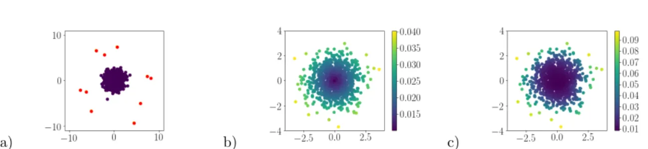
−1.5 −1.0 −0.5 0.0 0.5 1.0 1.5 −1 0 1 x1 x2
Figure 1. It is possible to construct a DPP with a (asymptotic) rebalancing property, meaning that it will sample several points from each cluster even when clusters are severely imbalanced. Here, we show three imbalanced clusters: two have size 2,000 and one has size 20. In blue, a sample from a polynomial DPP (see text for definition): it samples from each cluster despite their very different sizes. The formal rebalancing property is illustrated in Fig. 2.
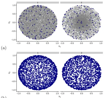
(a) 1 2 −1.0 −0.5 0.0 0.5 1.0 −1.0 −0.5 0.0 0.5 1.0 −1.0 −0.5 0.0 0.5 1.0 x1 x2 (b) 1 2 −1.0 −0.5 0.0 0.5 1.0 −1.0 −0.5 0.0 0.5 1.0 −1.0 −0.5 0.0 0.5 1.0 x1 x2
Figure 2. An illustration of the rebalancing result. (a) We sample ground sets (grey points) from two different distributions on the disc. In blue, two realisations of a polynomial DPP constructed from the ground set. Note how similar the two realisations are (density-wise), despite the very different ground sets they are drawn from. (b) We overlay 30 realisations of each DPP: the two resulting densities are very similar, again despite
the different ground sets. Our result states that they should indeed converge in largen and m, and that the
limiting density depends only on the shape of the domain. Here points close to the boundary are oversampled relative to points in the center, as predicted.
even in datasets where some clusters are much smaller than others. The result is illustrated in Figs. 1 and 2.
In a nutshell, the result is as follows. Suppose that the data X is a set ofn elements drawn iid from a continuous distributionµdefined on Ω⊂Rd. Build a projective DPPS of sizembased on the monomials of the xi’s (see Section 3.3.1 for a precise definition). Under mild regularity assumptions
onµ, we show that the intensity measure ofS, marginalized overX isindependent ofµ. Our proof is based on a powerful theorem from [37].
Note that this rebalancing property also occurs for iid sampling with sensitivities (that provide a sort of density estimation: the lower the density of points around xi, the larger σi, the higher the
chance of sampling it). What is noteworthy here is that the rebalancing property occurs “naturally”: without any sort of prior density-like estimation. We will emphasize this important point at the end of this Section.
In Section 3.3.1, we present the specific type of polynomial DPPs for which our proof holds, that are similar to those used in [38]. Our result is then formally stated in Section 3.3.2.
3.3.1. Projective polynomial DPPs
The L-ensemble we shall build is based on the first m monomials. In dimension one this is easy to define, so we start there and generalize later to dimension d > 2. For d = 1, we denote by X ={x1, . . . , xn}the original set (supposed to be drawn iid fromµdefined on Ω), and form then×m
Vandermonde matrix
(39) V(X) = [xji−1]n,mi,j=1 ∈Rn×m.
Note that this matrix has rankma.s. (asµis supposed regular enough) and contains all monomials up to degreem−1. TheL-ensemble we consider equals:
(40) L=VV>∈Rn×n.
The orthogonal polynomials (defined on Ω) under the empirical measuredµn= (1/n)Pδxi associated
to X, are defined in the usual manner, i.e. q0(x) of degree 0, q1(x) of degree 1, . . . such that: R
qi(x)qj(x)dµn=δij and
R xiq
j(x)dµn = 0 ifi < j. In other words, the sequence is constructed from
Gram-Schmidt orthogonalisation under dµn. Let us write qj(X) = (qj(x1), . . . , qj(xn))> ∈ Rn the vector consisting of the polynomialqj(x) taken at values inX. It is well-known (and easily verified)
that the QR decomposition ofVverifies:
V=QR (41)
withQ= (q0(X)|. . .|qm−1(X))∈Rn×mandR∈Rm×man upper triangular matrix.
Now, consider them-DPPSwithL-ensembleL=VV>. Using the fact that det(AB) = det(A) det(B) ifAandB are square, we have:
P(S) =Z−1det(LS)
=Z−1det((QRR>Q>)S)
=Z−1det((QQ>)S) det(R)2
=Z0−1det((QQ>)S)
such thatS is also am-DPP with L-ensembleQQ>. AsQ>Q =Im, i.e., QQ> is projective,S is in
fact a projective DPP. As a result, its associated marginal kernel is alsoQQ> (see Lemma. 2.7) and, for instance: (42) P(xi∈ S) = m−1 X j=0 qj2(xi).
The extension tod >1 is mostly straightforward, but there are a few differences to keep in mind when defining the Vandermonde matrix of monomials. Monomialsxα are now defined as:
(43) xα=
d
Y
j=1 x(j)αj
The total degree of a monomial equals the sum of the degrees in each variable, i.e. P
αi =||α||1.
is more than one monomial of total degreeφ. For example, in dimension 2, x = (x(1), x(2))> and the monomials of degree 2 are given by the powers (2,0), (0,2) and (1,1): x(1)2, x(2)2, x(1)x(2). A good way of thinking about the construction of a polynomial DPP in the multidimensional case is to pick first a maximum order (e.g. φ = 3), meaning that all monomials with total degree up to 3 are included. Then the natural sample size m for the DPP equals the total number of features, giving m = d+φφ
. Again, for d= 2 and φ = 3, this givesm = 1 + 2 + 3 + 4 = 10. In fact, there is one monomial of order 0: 1, two monomials of order 1: x(1) and x(2), three monomials of order 2 (the ones stated above), and four monomials of order 3: x(1)3, x(2)3,x(1)2x(2) and x(1)x(2)2. This implies that in dimensiond, the m-DPP detailed earlier is well-defined only for specific values ofm: m= d+11 =d+ 1, orm= d+22 = 1 2(d+ 1)(d+ 2), orm= d+3 3 =1 6(d+ 1)(d+ 2)(d+ 3), etc. A slight technical difficulty arises in defining the orthogonal polynomials of a multivariate measure: in dimension 1, the fact that there is a single monomial of a given degree leads to a natural order in which to perform the Gram-Schmidt procedure. In higher dimensions the order is only a partial order, so that we can introduce the monomials by blocks of equal degree, but within a block the ordering is arbitrary. So we may pick any arbitrary order (e.g. lexicographic) and run Gram-Schmidt in that order (for more see [39]). Given this choice the QR decomposition remains well-defined and all properties given above in the 1D case carry over to the general case. In particular, the link with the orthogonal polynomials on the discrete measureµn stays valid.
3.3.2. The rebalancing theorem
Formally, the result is as follows. The intensity functionι(x) of a point process quantifies the expected number of points to be found aroundx. We characterize the asymptotics of the intensity function of a DPP S when bothS and the ground setX are large, and show that, in that limit, the intensity is independent of the measureµfrom whichX is sampled from.
The result is stated formally as a double limit, letting first n go to infinity (an easy discrete-to-continuous limit), and then increasing the orderφof the polynomial DPP, which implies mgoing to infinity too. We emphasize that, empirically speaking, rebalancing occurs for reasonable values ofn andmbut the rate of convergence is hard to quantify.
Certain regularity assumptions are inherited from [37], to which we refer for more thorough details. The formal assumptions are as follows:
1) The initial datasetX ={x1, . . . , xn}is drawn i.i.d. from a measureµover a compact, convex4
domain Ω⊂Rd.
2) µand the Lebesgue measureνare mutually absolutely continuous on Ω, so thatµ0, the density, is well-defined everywhere on the domain (we use the Lebesgue measure for simplicity, another measure may be substituted)
3) We are interested in convergence “in the bulk”, ie. inside the domain. Formally, the results hold forD⊂D1⊂Ω, whereD is compact andD1 is open
4) µ0 is bounded above and below onD1
5) We form a m-DPP S on the set X, with a polynomial kernel of degree φ (defined in the previous Section), such thatm= φ+φd
.
6) (technical) µis regular in the sense of Stahl, Totik, and Ullman, and the Christoffel function with respect to µverifies condition (1.7) in [37].
The intensity measure of S, marginalizing overX, which we denote by In,φ(A) equals the expected
number of points ofS in setA, i.e.:
(44) In,φ(A) =EX,S(|S ∩ A|) =EX,S ( X s∈S I(s∈ A) )
Note that the expectation is overboth X andS. Furthermore,In,φ(Ω) equalsm, the total number of
points inS.
Our result may be stated as follows.
Theorem 3.9. Under the assumptions above, for all A ⊂D1, (45) lim φ→∞ 1 φ+d φ nlim→∞In,φ(A) = Z A κ(y)dy whereκis a density independentofµ
The proof is in Appendix C.
Lemma 3.10. κis mostly dependent on the distance to the boundaries ofΩ. For example, ifΩis the unit ball inRd,κ(y) =1− ||y||2−1/2
See [37] for a proof.
Several important remarks are in order:
• unlike iid sampling with sensitivities or other density-related measure for which such rebal-ancing property will also occur, there is here no prior density estimation: the L-ensemble is defined via the Vandermonde matrix that is trivial to compute. Thus, this rebalancing is a property that “naturally” arises from the DPP.
• this is only an asymptotic result asnand mgo to infinity. Finding minimal values of mfor which rebalancing is highly probable, or even rates of convergence is likely a difficult endeavour. We emphasize nevertheless that, empirically speaking, rebalancing occurs for reasonable values ofnandm, as visible in Figs. 1 and 2.
This ends the theoretical results of this paper. We now move on to applications. In the next Section, we apply the results to two problems: k-means and linear regression. In Section 5, implementation details are provided. Finally, experimental validation on artificial and real-world datasets is provided in Section 6.
4. Application to two problems:
k
-means and linear regression
We focus on two problems: k-means and linear regression. Admittedly, these are not the best problems to exhibit the usefulness of coresets: there already exists very efficient algorithms to solve them and the need for a controlled summary is in fact rare. We nevertheless focus on these two problems as they have been well studied in the iid setting, which it is our goal to improve on. Moreover, we derived analytical formulas for the sensitivity in the 1-means and the linear regression settings: we will thus be able to compare, in those two cases, DPP sampling vs the ideal iid setting (later in the experimental Section 6).
4.1. Application tok-means
The theoretical results of Section 3 are valid for any learning problem of the form detailed in Sec-tion 2.1. We now specifically consider thek-means problem on a set X comprised ofn datapoints in Rd. This problem boils down to findingkcentroidsθ= (c1, . . . , ck), all inRd, such that the following cost is minimized: L(X, θ) = X x∈X f(x, θ) with f(x, θ) = min c∈θkx−ck 2 .
Let ρbe the diameter of the minimum enclosing ball of X (the smallest ball enclosing all points in X). Theorem 3.1 and its corollaries are applicable to thek-means problem, such that:
Corollary 4.1 (m-DPP for k-means). Let S be a sample from an m-DPP with L-ensemble L. Let , δ∈(0,1)2. With probability at least 1−δ,S is a-coreset provided that:
m>m∗=32 2 max i σi ¯ πi 2 kdlog 24ρ2 hfiopt + 1 + log4 δ , (46) with∀i,¯πi=πi/m.
Setting the marginal probabilities to their optimal valuesπi=mσi/S,S is a -coreset with
proba-bility larger than 1−δprovided that: m> 32 2S 2 kdlog 24ρ2 hfiopt + 1 + log4 δ .
Proof. Let us write B the minimum enclosing ball of X, of diameterρ. The potentially interesting centroids are necessarily included inBsuch that the space of parameters Θ in thek-means setting is the set of all possiblek centroids inB: Θ =Bk. The metricdΘ we consider is the Hausdorff metric
associated with the Euclidean distance: ∀θ, θ0, dΘ(θ, θ0) = max max c∈θ cmin0∈θ0kc−c 0k 2, max c0∈θ0minc∈θkc−c 0k 2 .
An 0-net of Θ. Consider ΓB an0-net of B consisting of (2ρ0 + 1)
d small balls of radius 0. Such a
covering indeed exists: see, e.g., Lemma 2.5 in [40]. Consider Γ = ΓkB of cardinality|Γ|= (2ρ0 + 1) kd.
Let us show that Γ is an0-net of Θ, that is:
∀θ∈ Bk, ∃θ∗∈Γ s.t. d
Θ(θ, θ∗)60.
In fact, considerθ= (c1, . . . , ck)∈ Bk. By construction, as ΓB is an0-net ofB, we have:
∀i= 1, . . . , k ∃c∗i ∈ΓB s.t. kci−c∗ik6
0.
Writingθ∗= (c∗1, . . . , c∗k)∈Γ, one has:
dΘ(θ, θ∗)60,
which proves that Γ is an0-net of Θ. The number of balls of radius0=hfiopt/6γsufficient to cover Θ is thusη= (h12fiργ
opt+ 1)
kd.
f(x, θ) isγ-Lipschitz with γ= 2ρ. Consider anyθ,θ0 and x∈ X. We want to show that: −γ dΘ(θ, θ0)6f(x,θ)−f(x, θ0)6γ dΘ(θ, θ0).
Let us write c= argmint∈θkx−tk2 the centroid inθ closest to xand c0 = argmint0∈θ0kx−t0k2 the
centroid inθ0 closest tox. Moreover, let us write ˜c0 = argmint0∈θ0kc−t0k
2
the centroid inθ0 closest toc. Note thatc0 and ˜c0 are not necessarily equal. By definition of c0, one has:
kx−c0k6kx−c˜0k, such that: kx−c0k2− kx−ck26kx−˜c0k2− kx−ck26k˜c0−ck26dΘ(θ, θ0). Thus: f(x, θ0)−f(x, θ) =kx−c0(x)k2− kx−ck2= (kx−c0k − kx−ck)(kx−c0k+kx−ck) 6(kx−c0k+kx−ck)dΘ(θ, θ0)62ρ dΘ(θ, θ0). Finally, nσmin>1, as shown by the second lemma of Appendix D.
Given all these elements, Theorem 3.1 and its subsequent corollaries are thus applicable to the
k-means setting and one obtains the desired result.
Note that, in the case of DPPs, one could apply Theorem B.1 to thek-means problem, and obtain similar results.
4.2. Application to linear regression
We now consider the linear regression problem: findθ ∈Rd such that a measured vectory ∈
Rn is closest toXθ whereX>= (x1|. . .|xn)∈Rd×n arendata points inRd. Let us writeXi= (yi, xi) and X ={X1, . . . , Xn}. The least squares estimator minimizes:
L(X, θ) =ky−Xθk22. By denoting
f(Xi, θ) = (yi−x>i θ)
2, (47)
one can thus write the least squares solution to the linear regression problem in the form of the problems investigated in this paper: the objective is to minimize the costLwithf a positive function:
L(X, θ) =ky−Xθk22= n X i=1 f(Xi, θ). (48)
We suppose that allxi are enclosed in the unit ball in dimensiondand that yi∈[0,1]. Moreover,
we suppose that the space Θ is bounded and enclosed in a d-dimensional ball B centered in 0 of diameterρ.
Even though we derived the analytical formulation of the sensitivity for linear regression (Lemma D.3), we were not able to show thatnσmin >1 in general. We thus have the following slightly more com-plicated result:
Corollary 4.2 (m-DPP for linear regression). Let S be a sample from an m-DPP withL-ensemble L. Let, δ∈(0,1)2. With probability at least 1−δ,S is a-coreset provided that:
m>max(m∗1, m∗2) (49) with m∗1=32 2 max i σi ¯ πi 2 dlog 12ρ(4ρ+ 2) hfiopt + 1 + log4 δ , (50) m∗2=32 2 1 n¯πmin 2 dlog 12ρ(4ρ+ 2) hfiopt + 1 + log4 δ (51) with∀i,¯πi=πi/m.
Setting the marginal probabilities to their optimal valuesπi=mσi/S,S is a -coreset with
proba-bility larger than 1−δprovided that: m>32 2 max S2, S 2 n2σ2 min dlog 12ρ(4ρ+ 2) hfiopt + 1 + log4 δ . Proof. The metricdΘ we consider is the Euclidean distance in dimensiond.
- An 0-net of Θ. Consider ΓB an 0-net of Bconsisting of (2ρ0 + 1)d small balls of radius 0. Such
a covering indeed exists: see, e.g., Lemma 2.5 in [40]. The number of balls of radius 0 =hfiopt/6γ sufficient to cover Θ is thusη= (h12fiργ
opt + 1)
d.
-f(X, θ) isγ-Lipschitz with γ= 4ρ+ 2. Consider anyθ,θ0,xi andyi. We want to show that:
(yi−x>i θ) 2−(y i−x>i θ 0)22 6γ2 kθ−θ0k2. In fact: (yi−x>i θ) 2 −(yi−x>i θ0) 22 = θ>xix>i θ−θ0>xix>i θ0−2yix>i (θ−θ0) 2 = 2θ0>xix>i + (θ−θ 0)>x ix>i −2yix>i (θ−θ0)2 62θ0>xix>i + (θ−θ0)>xix>i −2yix>i kθ−θ0k 2 6 2xix>i kθ0k+ xix>i kθ−θ0k+ 2yikxik 2 kθ−θ0k2 (52)
by triangular inequality and writingxix>i
the 2-norm of the matrixxix>i , which is equal tokxik
2
and bounded by one by hypothesis. As Θ is supposed to be enclosed in a ball of radiusρ, we further have:
(yi−x>i θ)2−(yi−x>i θ0)2
2
6(4ρ+ 2)2kθ−θ0k2 (53)
Given these elements, Theorem 3.1 is applicable to the linear regression setting and one obtains
the desired result.
5. Implementation
5.1. The DPP’s ideal marginal kernel
Following the theoretical results, the ideal strategy (although unrealistic) to build the marginal kernel K of the ideal DPP sampling scheme would be as follows. 1/ Deal with outliers as explained in Appendix E untilσmax is not too large. 2/ Compute allσi. 3/ Set allπitomσi/Swithmsufficiently
large as detailed in the theorems. 4/ Find all non-diagonal elements ofKin order to minimize for all θthe estimator’s variance, as derived in Eq. (28):
Var( ˆL) =X i 1 πi −1 f(xi, θ)2− X i6=j K2ij πiπj f(xi, θ)f(xj, θ). (54)
while constraining K to be a valid marginal kernel, i.e.: SDP with 0 K 1, 5/ sample a DPP with kernel K. On our way to derive a practical algorithm with a linear complexity in n, many obstacles stand before us: there is no known polynomial algorithm to compute all σi in the general
setting, solving exactly the minimization problem of step 4 under eigenvalue constraint remains open, and sampling from this engineered ideal K costs O(n3) number of operations (see Alg. 1 of [8]: it necessitates a full diagonalization of K). Designing a linear-time algorithm that provably verifies under a controlled error the conditions of our previous theorems is out-of-scope of this paper. In the following, we prefer to first recall the intuitions behind the construction of a good kernel, and then discuss two choices of kernel we advocate: a Gaussian kernel and a Vandermonde-based kernel. 5.2. A first choice: the Gaussian kernel
In order forKto be a good candidate for coresets, it needs to verify the following two properties: • As indicated by the theorems, the diagonal entries Kii should increase as the associated σi
increases.
• As indicated by the variance equation, off-diagonal elements should be as large as possible (in absolute value) given the eigenvalue constraints. In fact, we cannot set all non-diagonal entries ofK to large values as the matrix’s 2-norm would rapidly be larger than 1. We thus need to choose the best pairs (i, j) for which it is worth setting a large value of Kij. A first glance
at the variance equation indicates that the largerf(xi, θ)f(xj, θ) is, the largerKij should be,
in order to decrease the variance as much as possible. Recall nevertheless that in the coreset setting, all sampling parameters should be independent ofθ. The off-diagonal elements should thus verify the following property: the larger is the correlation betweenxi and xj (the more
similar aref(xi, θ) andf(xj, θ) for allθ), the largerKij should be.
We show in the following in what ways the choice of marginal kernel K=L(I+L)−1
withLthe Gaussian kernel matrix with parameterτ: ∀(i, j) Lij = exp−
kxi−xjk2
2τ2 ,
is a good candidate to build coresets fork-means (the linear regression case is discussed later). Let us write U= (u1|. . .|un) the orthonormal eigenvector basis ofL and Λ= diag(λ1|. . .|λn) its diagonal
matrix of sorted eigenvalues, 0 6 λ1 6 . . . 6 λn. U and Λ naturally depend on τ. One shows for
instance that, with respect toτ, λn is a monotonically increasing function between 1 andn.
Concerning the off-diagonal elements ofK, let us first note that ifxiandxj are correlated (that is,
in thek-means setting, if they are close to each other), then Kij = X k λk 1 +λk uk(i)uk(j)
should be large in absolute value. In fact, in the limit where xi = xj, then ∀k, uk(i) =uk(j) and
Kij =Kii =Kjj. The determinant of the 2×2 submatrix ofK indexed by i andj is therefore null:
sampling both will never occur. Thus, the closer arexi and xj, the lower is the chance of sampling
both jointly. Moreover, ifxi andxj are far from each other (for instance, in different clusters), then
the entriesiandjofL0seigenvectors will be very different. For instance, say the dataset contains two well separated clusters of similar size. If the Gaussian parameterτ is set to the size of these clusters, then the kernel matrixLwill be quasi-block diagonal, with each block corresponding to the entries of each cluster. Also, each eigenvectoruk will have energy either in one cluster or the other such that
Kij is necessarily small if iandj belong to different clusters, and the event of sampling both jointly
is probable.
Concerning the probability of inclusion ofi, we have: Kii= X k λk 1 +λk vi(k)2,
where vi is the vector of sizen verifying ∀k, vi(k) =uk(i). For all i, kvik
2
= 1. The probability of inclusion is thus directly linked to the values ofkthat contain the energy ofvi: the more the energy
of vi is contained on high values of k, the larger is the probability of inclusion. Say we are again
in a situation where the clusters and the choice of Gaussian parameter τ are such that L is quasi block diagonal. Within each block, the eigenvector associated with the highest eigenvalue corresponds approximately to the constant vector. These eigenvectors being normalized, the associated entry of vi(k) is thus approximately equal to 1/
√
#Ci where #Ci is the size of the cluster containing dataxi.
Typically, if the cluster is small, that is, if #Ci tends to 1, the associated entry vi(k) tends to 1 as
well, such that all the energy ofvi is drawn towards high values ofk, thus increasing the probability
of inclusion of i. In other words, the more isolated, the higher the chance of being sampled. This corresponds to the intuition one may obtain for the sensitivityσi. It has indeed been shown that the
sensitivity may be interpreted as a measure of outlierness [26].
In the linear regression case, a similar argumentation is possible, up to the fact that pointican be an outlier from the point of view ofxiand/oryi, such that the kernel should take both into account:
we suggest the Gaussian kernel in dimensiond+ 1: ∀(i, j) Lij = exp−
kzi−zjk2
2τ2 ,
withzi= [x>i , yi]> ∈Rd+1.
In both contexts, we thus advocate to sample DPPs via a Gaussian kernelL-ensemble. We now move on to detailing an efficient sampling implementation.
5.2.1. Efficient implementation
Sampling exactly a DPP from the GaussianL-ensemble verifying ∀(i, j) Lij= exp−
kxi−xjk2 2τ2
consists in the following steps: 1) ComputeL.
2) DiagonalizeL in its set of eigenvectors{uk}and eigenvalues {λk}.
Algorithm 1The Gaussian kernel coreset sampling heuristics
Input: X ={xi}a set ofnpoints inRd, a Gaussian kernel parameterτ, a number of samplesm
·Drawr>O(m) random Fourier vectors associated to the Gaussian kernel with parameterτ
·Compute the associated RFF matrixΨ∈R2r×n as explained in Appendix F.1
·ComputeC=ΨΨ>∈R2r×2r the dual representation
·Compute the eigendecomposition ofC: obtain eigenvectors{vk}and eigenvalues{νk}
·Draw a sampleS from am-DPP withL-ensembleL=Ψ>Ψas explained in Appendix F.3.
· Compute the marginal probabilities πs for all xs ∈ S as explained in Appendix F.3, and set
weightsω(xs) = 1/πs.
Output: {S, ω} a weighted sample of sizem.
Step 1 costsO(n2d), step 2 costsO(n3), step 3 costsO(nµ3), where we recall thatµis the expected number of samples of the DPP. This naive approach is thus not practical. We detail in Appendix F how to reduce the overall complexity toO(nµ2), by 1/ taking advantage of Random Fourier Features (RFF) [41] to estimate a low dimensional representation Ψ ∈ R2r×n of the L-ensemble L ' Ψ>Ψ,
whereris the chosen number of features; and 2/ running a DPP sampling algorithm adapted to such a low rank representation.
In the experimental section, we will concentrate on m-DPPs as they are simpler to compare with state of the art methods that all have a fixed known-in-advance number of samples. The overall m-DPP sampling algorithm adapted to the k-means problem that we will consider is summarized in Alg. 1: given the dataX, the number of desired samplesm, and the Gaussian parameterτ, it outputs a weighted set of m samples S that is a good candidate to be a coreset if m is large enough. The runtime to buildΨisO(ndr); to computeCand diagonalize it isO(nr2); to sample am-DPP given this dual eigendecomposition isO(nm2). Given thatris set to a few timesm, the overall runtime of Alg. 1 isO(ndm+nm2).
Given a number of samplesmto draw, how should one set the Gaussian parameterτ? The larger is τ, the more repulsive is the m-DPP, and the smaller is the numerical rank of Ψ (the number of eigenvaluesν such thatnν is larger than the machine’s precision). Now, numerical instabilities arise while sampling an m-DPP if the numerical rank of Ψdecreases below m: τ should not be set too large. Also, the smaller isτ, the closer isLto the identity matrix, such that the closer is them-DPP to uniform sampling without replacement: τ should not be set too small. We will see in the following experimental section how the choice ofτ affects results.
5.3. A second choice: a projective DPP based on the Vandermonde matrix
A second choice of DPP sampling, that derives from our analysis, is the projective DPP withmsamples from theL-ensembleL=VV> whereVis the Vandermonde matrix (discussed in Section 3.3.1). This choice has several advantages over the Gaussian kernel:
• V takes O(nm) operations to compute: the overall m-DPP sampling cost is thus naturally O(nm2), with no need for any approximation technique.
• no particular scaleτ is introduced.
This choice however has the drawback that in dimension higher than 1, not all values ofmare allowed (only values ofmfor which there existsφ∈Ns.t. m= φ+φd
), as explained at the end of Section 3.3.1.
6. Experiments
6.1. Different strategies to compare...
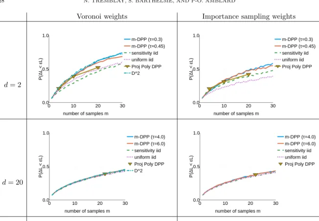
We will empirically compare results obtained with the five following approaches: 1) m-DPP: The strategy summarized in Alg. 1.
Algorithm 2The Vandermonde-based coreset sampling heuristics Input: X ={xi}a set ofnpoints inRd, a number of samplesm
·mshould verify: ∃φ∈Nsuch thatm= φ+φd .
·Compute the Vandermonde matrixV∈Rn×m.
· Compute the (Q∈ Rn×m,R∈ Rm×m) decomposition of V: V= QRwith Q>Q =Im and Ran
upper triangular matrix.
·Draw a sampleS from a projective DPP withL-ensembleL=QQ> as explained in Algorithm 3.
·Compute the marginal probabilitiesπsfor allxs∈ S withπs=kQ(s,:)k
2
the energy of thes-th line ofQ; and set weightsω(xs) = 1/πs.
Output: {S, ω} a weighted sample of sizem.
3) matched iid : An iid sampling strategy with replacement, matched to either m-DPP or PolyProj-DPP (depending on the context). More precisely, m samples are drawn iid with replacement, the probability of selecting xi at each draw being set topi=πi/m, whereπi is
the marginal probability of drawing xi inm-DPP (orPolyProj-DPP).
4) uniform iid: Uniform iid sampling with replacement.
5) sensitivity iid: The current state of the art iid sampling based on a bi-criteria approxi-mation to upper bound the sensitivity (Alg. 2 of [16]), or, if available (for instance in the case of 1-means and linear regression), an analytical formula of the sensitivity.
For the three iid methods (methods 3, 4 and 5), we will use the importance sampling estimator adapted to iid sampling of Eq. (9). For methods 1 and 2, we will use the importance sampling estimator adapted to correlated sampling of Eq. (16).
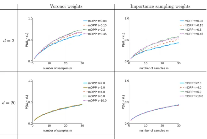
Empirically, when the ambient dimensiondis small, performance of all methods is enhanced if the weights in ˆLare set via Voronoi cells rather than set to inverse probabilities: given the sampleSof size m, compute its Voronoi tessellation inmcells, and associate to each samplexsa weightω(xs) equal
to the number of datapoints in its associated Voronoi cell. We will call the associated cost estimators ˆ
Lthe Voronoi estimators.
For completeness, we compare all these methods with another negatively correlated sampling method calledD2-sampling (commonly used fork-means++ seeding [42]):
6) D2 : sample the first element of S uniformly at random. Each subsequent element of S is drawn according to a probability proportional to the squared distance to the closest of the already sampled elements. The marginal probabilities are not known in this algorithm, so we will only be able to build the associated Voronoi cost estimator.
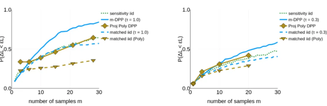
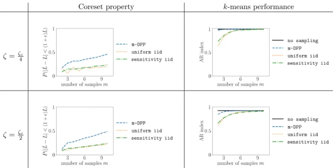
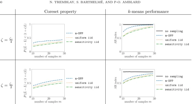
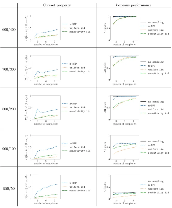
To measure the performance of each method, we will empirically estimate the probability that, given the method’s sampled weighted subset, it verifies the coreset property of Eq. 6 for a given randomly chosen θ (setting to 0.1). On the artificial data models we investigate, we estimate this probability via 50 randomly chosenθon 1000 realizations of the data. On the real-world datasets, we estimate this probability via 5000 randomly chosenθ. We will in general plot this probability versus the number of samples: the closer it is to 1, the better the sampling method for coresets.
In Sections 6.2.2 and 6.2.3, we will not only compare the coreset property of the samples obtained by each method, we will also compare the result of Lloyd’s classicalk-means heuristics [29] performed on the entire data versus the result obtained on the weighted samples of each method. To be precise, once thek-means heuristics on the weighted subset outputskcentroids, we classify all nodes (sampled or not) according to their closest distance to the centroids: this gives us a partition that we then compare using the Adjusted Rand (AR) similarity index [43] to the ground truth associated to the dataset. The AR index is a number between−1 and 1: the closer it is to 1, the closer are the partitions, the better the sampling method.