Theses and Dissertations Graduate School
2014
Management's Aggressiveness and Fair Value
Accounting: An Examination of Realized and
Unrealized Gains and Losses on ASC 820 Level 3
Assets
Robson Glasscock
Follow this and additional works at:http://scholarscompass.vcu.edu/etd Part of theBusiness Commons
© The Author
This Dissertation is brought to you for free and open access by the Graduate School at VCU Scholars Compass. It has been accepted for inclusion in Theses and Dissertations by an authorized administrator of VCU Scholars Compass. For more information, please contactlibcompass@vcu.edu.
Downloaded from
MANAGEMENT’S AGGRESSIVENESS AND FAIR VALUE ACCOUNTING: AN EXAMINATION OF REALIZED AND UNREALIZED GAINS AND LOSSES ON ASC 820
LEVEL 3 ASSETS
A Dissertation submitted in partial fulfillment of the requirements for the degree of Doctor of Philosophy in Business at Virginia Commonwealth University
by
Robson Glasscock, CPA
M.S. Accountancy, University of Denver, 2008 B.B.A. Accounting, Texas State University, 2003
Director: Myung Seok Park, Ph.D. Robert L. Hintz Professor of Accounting
Carolyn Strand-Norman, Ph.D.
Professor and Chair of the Accounting Department Benson Wier, Ph.D.
Professor of Accounting Jack Dorminey, Ph.D. Assistant Professor of Accounting
David Harless, Ph.D. Professor of Economics
Virginia Commonwealth University Richmond, Virginia
Acknowledgement
I would like to thank Pranav Ghai and Alex Rapp of Calcbench, Inc. for providing me with XBRL data consisting of realized and unrealized gains and losses on Level 3 assets. Without their generosity this dissertation would have been much more difficult to execute. The members of my dissertation committee (Dr. Myung Park, Dr. Jack Dorminey, Dr. Dave Harless, Dr. Carolyn Norman, and Dr. Benson Wier) have been selfless in their efforts to help turn my rough idea into a viable dissertation. I am grateful to each of you. I would also like to thank Michael McKenzie and Bryan Turner for answering questions, often during busy season, and helping me to keep the practitioner’s perspective in mind and not to forget my auditing roots. Thank you also to my dad, R. E. Glasscock, and my wife, Marisa Roczen, for keeping me grounded. I would not have been able to make it into the Ph.D. program without the former and would not have been able to make it out of the Ph.D. program without the latter. Lastly, I promise that I will always be as patient with students during office hours as Dr. Dave Harless, Dr. Oleg Korenok, and Dr. Leslie Stratton were with me.
Table of Contents
Abstract ………...v
I. Introduction ... 1
II. Literature Review and Hypothesis Development ... 7
Literature on Fair Value ... 7
Literature on Aggressiveness ... 10
III. Research Design... 15
Sample Selection ... 15
Dependent Variable ... 24
Independent Variables of Interest ... 25
Absolute Value of Discretionary Accruals ... 25
Composite Real Activities Manipulation ... 28
Meet-or-Beat Analysts’ Consensus Forecasts ... 30
Control Variables ... 31
Empirical Model ... 33
IV. Results ... 34
Descriptive Statistics ... 34
Multivariate Results ... 44
Discretionary Accruals and FVE ... 46
Real Activities Manipulation and FVE ... 49
Meet-or-Beat and FVE ... 49
Additional Analyses- Suspect vs. Non-suspect firms ... 52
Suspect Firm Analyses- FVE ... 53
Suspect firm analysis- Unrealized gains/losses ... 56
Additional Analyses- Unrealized Gains/Losses ... 59
V. Conclusion ... 62
Appendix A: Simultaneity Between FVE and DA ... 64
Appendix B: Comparison of Firms with Level 3 Instruments to COMPUSTAT ... 67
References ... 69
List of Tables
Table 1: Initial Sample of XBRL and Hand-Collected Data ………. 17
Table 2: Reconciliation of Hand-Collected Sample to Total Observations in Each Model ... 20
Table 3: Sample Industry Membership and Level 3 Instrument Types .……… 24
Table 4: Descriptive Statistics ……… 40
Table 5: Correlation Matrix ……… 43
Table 6: Multivariate Regressions .………. 51
Table 7: FVE Suspect Firm Analysis ..……… 55
Table 8: Unrealized Gain/Loss Suspect Firm Analysis ...……… 58
Table 9: Unrealized Gain/Loss Multivariate Regressions …………...……… 61
Abstract
MANAGEMENT’S AGGRESSIVENESS AND FAIR VALUE ACCOUNTING: AN
EXAMINATION OF REALIZED AND UNREALIZED GAINS AND LOSSES ON ASC 820 LEVEL 3 ASSETS
By Robson Glasscock
A Dissertation submitted in partial fulfillment of the requirements for the degree of Doctor of Philosophy in Business at Virginia Commonwealth University
Virginia Commonwealth University, 2014
Director: Myung Seok Park, Robert L. Hintz Professor of Accounting
Prior research has shown that even the most subjective fair value estimates are value-relevant (Song et al. 2010, Kolev 2009, Goh et al. 2009) and that managers appear to use Level 3 valuations opportunistically (Valencia 2011, Fiechter and Meyer 2009). However, the
association between “traditional” measures of aggressiveness in financial reporting and biased estimates of fair value has not been previously studied. I test whether aggressiveness, as measured by discretionary accruals, real activities manipulation, and meeting-or-beating analysts’ consensus estimates, is positively associated with realized and unrealized gains and losses on Level instruments. Overall, I find limited support that aggressive firms
opportunistically use fair value measurements to overstate earnings. Inferences remain the same whether only the unrealized component of gains/losses are examined and whether firms are classified into “suspect” or “non-suspect” groups.
I.
Introduction
On May 12, 2011, the Financial Accounting Standards Board (FASB) issued a press release stating that the FASB and the International Accounting Standards Board (IASB) completed a significant milestone in the process of moving towards a single, global set of high-quality financial accounting standards. Specifically, the boards issued common standards regarding techniques and disclosures related to fair value accounting. The promulgation of common standards is known as “convergence”, and the boards have been actively working to align US Generally Accepted Accounting Principles (GAAP) and International Financial Accounting Standards (IFRS) since 2002. Due to convergence, understanding the risk and benefits of reporting assets and liabilities at fair value literally has global implications. Leslie Seidman, Chairman of the FASB, said, “This Update represents another positive step toward the shared goal of globally converged accounting standards. Having a consistent meaning of the term ‘fair value’ will improve the consistency of financial reporting around the world” (FASB 2011).
Despite the world-wide importance of fair value accounting, relatively little empirical evidence exists regarding the current fair value standards. This sentiment is expressed by
DeFond (2010), “Going forward, I think there are accounting developments on the horizon about which we know relatively little, and hence are logical prospects for future research. One
example is fair value accounting, which represents a potentially sea-changing development in the accounting environment” (DeFond 2010, 11). Further, the additional disclosures required by modern fair value standards may be able to provide further insights into issues that have been debated in prior research. Barth and Taylor (2010) are critical of the conclusions made by Dechow, Myers, and Shakespeare (2010) regarding the manipulation of fair value estimates
during asset securitizations stating that, “Recent changes in accounting standards might provide a greater opportunity to investigate the discretion in fair value estimates. For example, SFAS 157 defines fair value, provides guidance on how to determine it, and requires more extensive
disclosures about fair value than required previously. Perhaps these new disclosures can be used to construct more direct tests” (Barth and Taylor 2010, 33).
Laux and Leuz (2009) discuss the major arguments for and against fair value accounting subsequent to the financial crisis. The authors frame the discussion within the tradeoff between relevance and reliability and state that accounting standards setters have debated this tradeoff for decades. Laux and Leuz (2009) write, “Few dispute that transparency is important. But the controversy rests on whether fair value accounting is indeed helpful in providing transparency and whether it leads to undesirable actions on the parts of banks and firms” (Laux and Leux 2009, 827-828). This study provides direct evidence regarding one such undesirable action (e.g., firms intentionally manipulating fair value estimates to manage earnings).
Prior to the passage of Statement of Financial Accounting Standards No. 157 (FAS 157), existing guidance related to fair value accounting remained dispersed through the
pre-codification hierarchy of Generally Accepted Accounting Principles (GAAP) in the United States. The definitions of fair value varied across standards, and specific implementation guidance was limited. The FASB recognized that these problems “… created inconsistencies that added to the complexity of applying U.S. GAAP” (FASB 2006, FAS 157-2). FAS 157 did not increase the scope of which account balances or classes of transactions were to be reported at fair value. Rather, FAS 157 was written to be a single authoritative implementation standard for other areas of US GAAP requiring fair value accounting.
The FASB implemented the Accounting Standards Codification (ASC) for financial reporting periods subsequent to September 15, 2009. The ASC technically supersedes all prior US GAAP, but many of the existing Statements of Financial Accounting Standards were
incorporated into the Codification. For instance, the provisions of FAS 157 are incorporated into the Codification as Accounting Standards Codification 820. Hereafter, this paper references the Accounting Standards Codification rather than the Statement of Financial Accounting Standards (ASC 820 instead of FAS 157).
Inputs to the three valuation techniques permitted by ASC 820 (i.e., market approach, income approach, or cost approach) are either deemed to be observable or unobservable. Observable inputs are defined as, “… inputs that reflect the assumptions market participants would use in pricing the asset or liability developed based on market data obtained from sources independent of the reporting entity” (FASB ASC 820-10-20). Unobservable inputs are defined as inputs which “… reflect the entity’s own assumptions about the assumptions market
participants would use in pricing the asset or liability developed based on the best information available in the circumstances” (FASB ASC 820-10-20 ).
ASC 820 also created a hierarchy of three levels for fair value measurement and
expanded the disclosures required for fair value measurements. Per ASC 820, Level 1 assets or liabilities use quoted market prices for identical assets or liabilities in active markets. Level 2 assets or liabilities use observable prices which are not included in the Level 1 classification. Examples of Level 2 observable prices are quoted prices for similar, not identical, assets or liabilities in active markets and quoted prices for identical or similar assets or liabilities in markets that are not deemed to be “active.” Level 3 items are commonly referred to as “mark-to-model” assets or liabilities. These assets/liabilities use the entity’s own assumptions as valuation
inputs and, accordingly, management has the most discretion over the valuation of Level 3 assets or liabilities. It is this category which uses inputs deemed to be “unobservable” per ASC 820 and, accordingly, additional disclosures are required.
Using ASC 820 disclosures, this study examines whether aggressive firms use their considerable discretion over the valuation inputs used in the Level 3 category to report biased (overstated) gains/losses for Level 3 assets. Specific examples of these assets include auction rate securities, investments in hedge funds, investments in private equity firms, collateralized debt obligations, credit default swaps, and derivatives relating to commodity basis differentials. Biased gains/losses may be either unrealized or realized. The unrealized gains/losses used in this study are attributable to Level 3 assets which are not designated as available-for-sale. These unrealized gains/losses are booked to income statement accounts and alter the current period’s earnings. The realized gains/losses attributable to Level 3 assets include assets which were designated as available-for-sale in a prior period but have been sold in the current period and sales of assets which were designated as trading securities. These realized gains/losses are booked to income statement accounts, alter the current period’s earnings, and provide management with a second way to use Level 3 assets to manage earnings.
In this study, I define a firm’s aggressiveness in its financial reporting using three different measures. Each measure has been used extensively in the accounting and finance literature. Aggressiveness is measured using the absolute value of lagged discretionary accruals, composite real activities manipulation, and “Street” earnings that are greater than or equal to analysts’ consensus estimates.
Findings from prior research are consistent with firms being rewarded for reporting earnings consistent with the market’s expectations (Skinner and Sloan 2002; Bartov, Givoly, and Hayn 2002). These findings provide aggressive firms with incentives to report overstated realized gains/losses on Level 3 assets. It is also known that the Level 3 items are value relevant (Song, Thomas, and Yi 2010; Kolev 2009; Goh, Ng, and Yong 2009). The fact that the market discounts, but still values, Level 3 items provides incentives to aggressive firms to willfully overstate Level 3 assets via the concurrent overstatement of unrealized gains/losses. It remains an open empirical question whether aggressive firms engage in these behaviors to a greater extent than nonaggressive firms. In this study, I predict that management’s aggressiveness (i.e., discretionary accruals, real activities manipulation, and propensity to meet or beat analysts’ consensus estimates) is positively associated with realized and unrealized gains/losses on Level 3 assets.
I find that realized and unrealized gains/losses on Level 3 assets are significantly associated with discretionary accruals in a variety of specifications. The relationship is significant at conventional levels regardless of the test. There is moderate support for the conjecture that realized and unrealized gains/losses on Level 3 assets and management’s aggressiveness are related when real activities manipulation is used as a proxy for
aggressiveness. However, I find little evidence of an between aggressiveness and realized and unrealized gains/losses on Level 3 assets when meeting-or-beating is used as the
operationalization of aggressiveness.
This study contributes to the post-FAS 157/ASC 820 fair value accounting literature in several ways. First, Valencia (2011) and Fiechter and Meyer (2009) provide evidence that fair value accounting is used as an earnings management tool conditional upon the properties of the
firm’s earnings. However, the relationship between fair value accounting and established measures of firm aggressiveness (e.g., discretionary accruals, real activities manipulation, and propensity to meet-or-beat analysts’ consensus estimates) has not been previously investigated. Both Valencia (2011) and Fiechter and Meyer (2009) conduct analyses where the primary explanatory variables are related to earnings, changes in earnings, or net income. Discretionary accruals, meeting-or-beating, and real activities manipulation are not considered by either study. Second, understanding whether aggressive firms intentionally report biased fair value estimates is important because both Valencia (2011) and Fiechter and Meyer (2009) report that higher-quality auditors and stronger corporate governance do little to constrain managers from using Level 3 fair value estimates opportunistically. Third, all of the modern (i.e., post FAS 157) fair value studies have examined fair value accounting using samples consisting solely of financial services firms. Financial services firms have unique operating and accounting environments, and findings supporting the notion that managers willfully overstate fair value estimates may not be generalizable to nonfinancial services firms. However, this study provides evidence that nonfinancial services firms also use fair value accounting as an earnings management tool. Fourth, Barth and Taylor (2010) are optimistic that the ASC 820 disclosures may be used to construct more direct tests of whether managers opportunistically abuse the discretion inherent in fair value estimates. This study includes several direct tests of the relationship between
management aggressiveness and fair value.
The remainder of this paper is organized as follows. Section II discusses prior literature and develops the hypothesis of this paper. Section III details the sample selection, variables, and empirical research design of the study. Section IV presents the results, and Section V discusses the conclusion.
II.
Literature Review and Hypothesis Development
Literature on Fair ValueFAS 157 has two implementation dates depending upon the type of assets/liabilities the firm has (financial vs. nonfinancial) and the frequency with which the firm reports the fair values of the assets/liabilities. For firms with financial assets/liabilities, or nonfinancial assets/liabilities that are reported at fair value with at least an annual frequency, FAS 157 became effective for financial statements filed with fiscal years beginning after November 15, 2007. For firms with nonfinancial assets/liabilities that are not reported at fair value on at least an annual basis, FAS 157 became effective for fiscal years beginning after November 15, 2008 (FSP FAS 157-2).
Much of the existing FAS 157 research focuses on financial services institutions. For example, working papers from Valencia, Fiechter and Meyer, Goh et al., and Kolev all study FAS 157 within the context of financial services firms. The concentration of fair value reporting within the banking industry is not limited to working papers. Recently published studies from Badertscher et al. (2012), Riedl and Serafeim (2011), and Song et al. (2010) also use samples consisting solely of financial services firms. The papers fall into two broad research categories. One group examines the value-relevance of fair value estimates and disclosures while the second attempts to determine if managers use their discretion over fair value in an opportunistic manner.
The value-relevance studies include Song et al. (2010), Kolev (2009), and Goh et al. (2009). Song et al. (2010) employ a modified version of the Ohlson (1995) model. Ohlson’s original model expresses share price as a function of book value and the present value of cumulative expected abnormal earnings. Song et al. (2010) decompose the book value of the firm into assets/liabilities carried at historical cost and the ASC 820 framework for
relationship between each asset/liability level and share price. Song et al. (2010) note that, theoretically, the regression coefficients for assets equal positive one and the regression
coefficients for liabilities equal negative one, but find that the estimated parameters decrease in absolute value as the fair value levels increase. This finding is consistent with investors placing less reliance on fair value adjustments that are subject to higher amounts of managerial
discretion. Kolev (2009) and Goh et al. (2009) use similar research designs and report findings1 consistent with Song et al. (2010).
Each of the value-relevance studies concludes that fair value estimates with less discretion are more value-relevant to investors, but all three fair value levels are significantly associated with share price. These findings are interesting because they show that even fair value disclosures with the most discretion (Level 3 assets/liabilities) are priced by capital markets. These findings give overly aggressive managers an incentive to report biased
(overstated) fair value estimates for Level 3 assets. Whether or not aggressive managers abuse the considerable leeway they have in determining the fair value of Level 3 assets remains an open empirical question.
Valencia (2011) and Fiechter and Meyer (2009) explore whether financial services institutions use Level 3 fair value estimates opportunistically. Valencia (2009) studies the amount of unrealized gains that banks recognized in earnings around the financial crisis of 2008.2 These unrealized gains are the result of changes in the valuations of Level 3 instruments between reporting periods. Valencia (2009) subtracts the unrealized gains from the actual earnings reported by the financial institutions. He shows that banks which would have reported
1
Goh et al. and Kolev both study the fair value of net assets which are defined as the total fair value assets for a given level minus the total fair value liabilities for the same level.
losses had they not been able to recognize the Level 3 valuation changes report unrealized gains that are higher than banks which would have reported positive earnings had they not been able to recognize the Level 3 valuation changes. These results also hold for banks which would have reported negative changes in earnings had they not been able to recognize Level 3 valuation changes. Taken together, these findings suggest that managers of financial services institutions use their discretion over Level 3 fair value estimates to report earnings that are positive and higher than prior reporting periods. Interestingly, Valencia (2009) finds no evidence that stronger corporate governance or more prestigious auditors constrains such behavior.
Fiechter and Meyer (2009) examine whether banks use the discretionary nature of Level 3 fair value estimates to smooth earnings. Unlike Valencia (2011), their sample consists of observations limited to the financial crisis of 2008. Fiechter and Meyer (2009) find a negative and statistically significant association between unrealized gains/losses on Level 3 instruments and net income before unrealized gains/losses on Level 3 instruments. They conclude that this is evidence consistent with firms using the subjectivity inherent in fair value estimation of opaque assets to smooth earnings (firms with higher earnings report lower unrealized gains/losses and vice versa). Similar to Valencia (2011), the findings of the authors do not indicate that stronger corporate governance mitigates the ability of managers to report biased fair value estimates.
Though Valencia (2011) and Fiechter and Meyer (2009) show that characteristics of both current earnings and current changes in earnings influence management’s use of ASC 820 Level 3 fair value estimates, the relationship between management’s aggressiveness and Level 3 reporting has yet to be studied. The research design used in the current study differs from both Valencia (2011) and Fiechter and Meyer (2009) in that management’s use of ASC 820 Level 3
fair value estimates are examined conditional upon the characteristics of the firm itself and not upon the characteristics of the firm’s reported earnings.
Literature on Aggressiveness
Teoh, Welch, and Wong (1998) attempt to explain the widely observed
underperformance of initial public offerings (IPOs) by separating firms into “aggressive” or “conservative” categories and testing for differences in the three-year returns of each group. They define aggressive IPOs as firms in the highest quartile of discretionary accruals and conservative IPOs as firms in the lowest quartile of discretionary accruals. Teoh et al. (1998) show that aggressive IPO firms cumulative buy-and-hold returns are between 15 to 30 percent lower than conservative IPO firms.
Kim and Park (2005) study aggressive (i.e., opportunistic) accounting decisions within the context of seasoned equity offerings (SEO). These issuances give managers two incentives to issue shares at higher prices. First, a higher price per share allows the firm to collect more cash for a given number of shares. Second, the firm must sell fewer shares to raise a particular amount of capital. This allows managers to prevent excess dilution of their equity ownership stakes in the firm subsequent to the issuance. Kim and Park (2005) hypothesize that managers of SEO firms will use their financial reporting discretion aggressively and will manage earnings to issue shares at inflated prices. They refer to this as the “issuer’s greed hypothesis” and
operationalize aggressiveness using discretionary accruals from the cross-sectional Modified Jones Model (1991). The findings of Kim and Park (2005) are consistent with the issuer’s greed hypothesis.
The use of discretionary accruals as a measure of firm aggressiveness is also accepted in the auditing literature. Francis and Yu (2009) examine the relationship between local office size and audit quality for clients audited by Big 4 auditors. They also use discretionary accruals as a proxy for aggressive financial reporting and conclude, “Clients audited by larger offices are also less likely to have aggressively managed earnings as evidenced by smaller abnormal accruals and a lower likelihood of meeting benchmark earnings targets… “ (Francis and Yu 2009, 1522). Further, Gunny and Zhang (2013) study the relationship between Public Company Accounting Oversight Board (PCAOB) inspections and audit quality. Gunny and Zhang (2013) state that an alternative explanation for their results is that the PCAOB may devote more time and resources inspecting auditors that allowed aggressive accounting choices in the past. Gunny and Zhang (2013) use a two-stage model to account for this and include accruals as a proxy for
aggressiveness.
However, discretionary accruals are not the only measure to gauge managers’ aggressiveness toward financial reporting. Management aggressiveness may also appear in operating decisions. Roychowdhury3 (2006) defines real activities manipulation as, “departures from normal operating practices, motivated by managers’ desire to mislead at least some
stakeholders into believing certain financial reporting goals have been met in the normal course of operations” (p. 337).
Roychowdhury (2006) defines suspect firm-years as observations where net income divided by total assets is greater than 0 and lower than .005. This definition is partially based
3
Roychowdhury cites a survey from Graham et al. (2005) in which executives stated that it was important to meet various earnings targets (i.e., prior period earnings, analyst forecasts, etc.). The executives surveyed also admitted that they were willing to manipulate day-to-day operating procedures to meet these targets.
upon Burgstahler and Dichev (1997) who document discontinuities in the distributions of both earnings and changes in earnings. Specifically, Burgstahler and Dichev (1997) find lower-than-expected frequency of observations immediately to the left of zero and higher-than-lower-than-expected frequency of observations immediately to the right of zero. They conclude that the
discontinuities in the distributions are attributable to earnings management. Other studies (Cohen, Dey, and Lys 2008; Kim, Park, and Wier 2012) also find that in suspect firm-years, firms report lower abnormal cash flow from operations, lower discretionary expenses, and higher abnormal production costs. Each of these findings is consistent with managers’ aggressiveness toward financial reporting.
Cohen et al. (2008) examine the relationship between accruals-based earnings
management and real activities manipulation. They find that passage of the Sarbanes-Oxley Act
of 2002 (SOX) significantly reduced the prevalence of accruals-based earnings management as
compared to real activities manipulation. These findings are not surprising given the requirements of Section 404 of SOX. Section 404 requires management and the auditors to opine on the adequacy of both the design and operating effectiveness of the company’s internal controls. A stronger internal control environment likely constrains accruals-based earnings management but may not necessarily reduce real activities manipulation. Cohen et al. (2008) conclude that accruals-based earnings management and real activities manipulation are substitutes for one another and that real activities manipulation became more prevalent
subsequent to SOX. This suggests that RAM could be a trait of aggressive financial reporting.
Cohen and Zarowin (2010) study the substitution effect between accruals-based manipulation and RAM within the context of seasoned equity offerings. They find that while SEO firms use both accruals-based earnings management and RAM, these two earnings
management mechanisms are substitutes for one another. These findings are similar to Cohen et al. (2008) but generalizable to a more specific subsection of firms (i.e., SEOs). Cohen and Zarowin (2010) conclude that the substitution choice manager make between these two types of earnings management partially depends upon auditor scrutiny and perceived litigation penalties.
The sample period of this study is constrained to the post-SOX period due to the effective date of ASC 820. The findings of Cohen, Dey, and Lys (2008) and Cohen and Zarowin (2010) suggest that an alternative measure of management aggressiveness may be warranted in the post-SOX period. Therefore, the composite real activities manipulation measure from Cohen and Zarowin (2010) is used as an alternative proxy for management’s aggressiveness.
Finally, meeting or beating analysts’ forecasts (MBE) is used as the third proxy for management’s aggressiveness in this study. Skinner and Sloan (2002) find that the return underperformance of growth stocks relative to value stocks is primarily explained by the asymmetric reactions of investors when growth stocks report negative earnings surprises. Negative earnings surprises are defined as fiscal quarters in which the firm’s actual earnings per share is less than the analyst consensus forecast of earnings per share. The evidence reported by Skinner and Sloan (2002) gives growth firms strong incentives to avoid negative earnings surprises, and thus, also incentivizes MBE behavior.
However, incentives to avoid negative earnings surprises are not confined to growth stocks. Bartov, Givoly, and Hayn (2002) use an initial sample containing all firms for which I/B/E/S estimates are available and conclude that cumulative abnormal returns are positively associated with MBE. They also report asymmetric market reactions depending upon the type of discrepancy between the firm’s reported numbers and analysts’ consensus estimates. For
example, the premium for meeting analysts’ forecasts is significantly different from the premium for beating analysts’ forecasts, and the absolute value of the premium to beating analysts’
forecasts differs from the penalty for failing to meet analysts’ forecasts. Bartov et al. (2002) also present evidence that the market still rewards MBE behavior in cases in which the market’s expectations were likely met via earnings management or analyst manipulation. These findings further incentivize aggressive firms to engage in MBE behavior.
Matsumoto (2002) finds that managers prefer pessimistic management earnings forecasts as a tool for MBE, Matsumoto’s results show that discretionary accruals and MBE are positively and significantly related. Therefore, I employ MBE as a third measure of management
aggressiveness in the current study.
The existing aggressiveness and fair value literature discussed above leads to several conclusions. The market often reacts positively in cases where it is likely that benchmarks are met via aggressive financial reporting practices by the firm, assets subject to the largest amounts of managerial discretion are still priced by capital markets participants, financial services
institutions use fair value to report earnings and changes in earnings that are positive, financial services institutions also use fair value to smooth earnings, and both auditors and stronger corporate governance by the board of directors are unable to constrain such behavior. Therefore, aggressive nonfinancial services firms are also likely to opportunistically report biased
(overstated) fair value estimates in an attempt to obtain the same positive reaction from the market. This provides support for the following hypothesis stated in alternate form:
H1: Management’s aggressiveness in financial reporting is positively associated with realized and unrealized gains/losses on Level 3 assets.
III. Research Design
Sample SelectionThe United States Securities and Exchange Commission (SEC) requires that large accelerated filers (i.e., firms with common equity market capitalization of at least $700 million) prepare their financial statements in an interactive data format using eXtensible Business Markup Language (XBRL) for reports filed on or after June 15, 2009. The SEC intended the XBRL format to be more useful to investors because XBRL “tagged” documents enable investors to quickly and easily download data directly into spreadsheets. The SEC stated that this should help investors analyze the data in a variety of ways using commercially available software (SEC 2009).
Calcbench Inc. uses cloud-based computing to process and store data from all eXtensible Business Reporting Language (XBRL) tagged financial reports filed with the United States Securities and Exchange Commission. The population of publicly traded firms with realized or unrealized gains/losses on Level 3 assets was obtained from Calcbench Inc. XBRL prepared documents are mandated beginning the second calendar quarter of 2009, but interpolation based on data in the 10-Q’s is possible. Therefore, the sample period in this study runs from the first calendar quarter in 2009 to the second calendar quarter of 2012. After interpolation there are 175 firms in the sample and 902 firm-quarters. Financial services firms (i.e., SIC codes 6000-6799) are excluded due to the extant research on financial services firms and fair value accounting. The remaining XBRL sample includes 105 firms and 492 quarters of which 410 firm-quarters report non-zero realized and unrealized gains/losses on Level 3 assets.
A recent white paper from Columbia University’s Center for Excellence in Accounting & Security Analysis outlines a series of problems in the current XBRL reporting environment.
Among the problems discussed by Harris and Morsfield (2012) are low-quality XBRL document tagging due to limited liability of fliers for errors combined with the fact that XBRL tagging is unaudited, filers utilizing incorrect XBRL tags, and errors causing the tagged data to not reconcile with the EDGAR filling. In fact, the first recommendation made by Harris and Morsfield (2012) is that the error rates of XBRL data be significantly reduced. Based on the findings of Harris and Morsfield (2012) data is hand-collected from EDGAR fillings (i.e., 10-Q’s and 10-k’s) for the 492 firm-quarters discussed above. The hand-collected data contains 86 firms and 378 firm-quarters of which 333 firm-quarters report non-zero realized and unrealized gains/losses on Level 3 assets. The XBRL data does not agree with the EDGAR fillings in nearly one third of cases (30.88%), and the hand-collected data is used for all of the reported descriptive statistics and empirical analyses.
The XBRL data provided by Calcbench, Inc. contains 1,409 firm-quarters and 231 unique firms. This data theoretically consists of the entire population of firms that recognize changes in Level 3 assets in earnings. However, due to the XBRL implementation issues previously
discussed it is likely that some firms with Level 3 gains/losses in earnings are absent. Excluding financial services firms (i.e., SIC codes 6000- 6799) eliminates 613 firm-quarters and 82 unique firms. It is worth noting that financial services institutions are the minority (35.50 %) of firms with Level 3 assets. XBRL tags exist for time periods beyond single quarters. For example, observations may contain cumulative figures for the first two or even three fiscal quarters. These cumulative periods are useful for interpolating4 values for missing time periods, but they are unsuitable for a research design using single-quarter financial data from COMPUSTAT.
4
Total realized and unrealized gains/losses included in earnings for two or more quarters is the sum of each single quarter. This may be seen in GE’s 3/31/2009 and 6/30/2009 10-Qs and SWN’s 3/31/2010 and 6/30/2010 10-Q’s. However, this relationship does not usually hold for unrealized gains/losses.
Cumulative annual figures are also present in the XBRL data and pose the same problem. Interpolating when possible and removing these cumulative periods results in a net decrease of 302 firm-quarters. This brings the initial XBRL sample to 492 firm quarters and 105 unique firms. Hand-collecting data from the EDGAR filings (e.g., 10-Q’s and 10-K’s) results in 378 firm-quarters and 86 unique firms. Table 1 details specific reasons that each observation is removed. The most common reasons for removal are 10-Q’s being prepared on a cumulative basis, lack of disclosure regarding whether total realized and unrealized gains/losses are booked to earnings or OCI, and missing observations in the panel which precludes interpolation.
Table 1
Initial Sample of XBRL and Hand-Collected Data
Observations
XBRL Data Obtained from Calcbench, Inc. 1,409
Less: Missing Value for Realized and Unrealized Gain/Loss Tag (1)
Duplicate Observation (1)
Financial Services Firms (613)
Cumulative 6-month and 9-month Data (282)
Annual Realized and Unrealized Data (212)
Add: Interpolated Observations 192
Initial XBRL Sample 492
Less: No Level 3 Rollforward Table in 10-Q/10-K (6)
Only Cumulative 6- or 9-Month Reported (33)
Total Realized and Unrealized Gains/Losses Not Reported (8)
OCI vs. Earnings Not Disclosed (11)
Foreign Filer Without Any 10-Q's/10-K's (6)
No 10-Q or 10-K Filed (5)
Interpolation Not Possible Due to Missing Observations in Panel (45)
Initial Hand-Collected Sample 378
COMPUSTAT data is necessary to estimate discretionary accruals, real activities
hand-collected data were accumulated in one file which was merged with COMPUSTAT-
Fundamentals Quarterly data using a one-to-one merge based on CIK, DATADATE, and FQTR. Fiscal period-end dates in COMPUSTAT (i.e., DATADATE) may be within several days from the actual period-end reported in EDGAR filings. The XBRL data contains the actual period-end reported in the EDGAR filling, and these dates are adjusted prior to the merge. Each observation in the XBRL data was successfully merged with COMPUSTAT.
One additional interpolation is necessary with Virginia Commonwealth University’s COMPUSTAT- Fundamentals Quarterly subscription. Quarterly cash flow (i.e., OANCFQ) is necessary to estimate both real activities manipulation and discretionary accruals. However, the VCU subscription contains OANCFY which is the cumulative cash flow across all reported quarters. In the first quarter OANCFQ equals OANCFY, but in subsequent quarters OANCFY will report the cumulative six-, nine-, and twelve-month cash flows. Differencing OANCFY based on fiscal quarter for Q2, Q3, and Q4 provides the single-quarter operating cash flow5.
Missing values in the COMPUSTAT- Fundamentals Quarterly data further reduce the 378 firms in the hand-collected sample. Gross property plant and equipment (i.e., PPEGTQ) is missing in 55.02 percent of the 153,912 firm-quarters covered by COMPUSTAT between January 1, 2009 and June 30, 2012. PPEGTQ is missing in 13.49 percent of the hand-collected observations, and this precludes estimation of both normal and discretionary accruals for these observations. Missing PPEGTQ values are much less frequent in the hand-collected
observations than in the population of firms covered by COMPUSTAT.
The estimation sample used to test the relationship between real activities manipulation and realized and unrealized gains/losses on Level 3 instruments is also reduced due to missing values. Quarterly selling, general, and administrative expenses (i.e., XSGAQ) is missing in 36.22 percent of the 153,912 firm-quarters covered by COMPUSTAT between January 31, 2006 and December 31, 2012. XSGAQ is missing in 42.06 percent of the hand-collected observations. This pattern is the opposite of the relative proportion of missing values between the population of firms covered by COMPUTAT and the hand-collected sample that was observed for
PPEGTQ. While PPEGTQ is missing in a much higher percentage of the complete COMPUSTAT data than the hand-collected sample, the opposite holds for XSGAQ. This precludes estimation of normal expenses, abnormal discretionary expenses, and real activities manipulation for nearly half of the hand-collected observations. The RAM variable is the most impacted by missing values because composite RAM is the sum of residuals from three separate regressions. RAM also requires a larger number of lags than DA and, unlike DA, seasonal differences are used to estimate RAM.
Table 2 provides reconciliations of the initial hand-collected observations to the number of observations included in each model. The sample used to test the relationship between MBE and FVE is least affected by missing values, and the sample used to test the relationship between RAM and FVE is most affected by missing values.
Table 2
Reconciliation of Hand-Collected Sample to Total Observations in Each Model
DA RAM MBE
Initial Hand-Collected Sample 378 378 378
Less: Missing Values- PPEGTQ (51) - -
Missing Values- XSGAQ - (159) -
Missing Values- Other (25) (15) (27)
Total Observations 302 204 351
Variables: DA is the absolute value of discretionary accruals in period t-1 estimated as in Dechow et al. 1995. RAM is composite real activities manipulation which is the sum of abnormal production minus abnormal cash flows from operations minus abnormal production. Each individual RAM element was estimated as in Cohen and Zarowin (2010). DA and RAM are both Winsorized at the 1% level. PPEGTQ is gross property plant and equipment, quarterly. XSGAQ is selling, general, and administrative expenses, quarterly. MBE is an indicator variable equal to one if the firm's "Street" earnings are greater than or equal to the latest analyst consensus estimates.
Analyst forecast data to calculate MBE is obtained from IBES via the Thomson Reuters Spreadsheet Link (TRSL) interface. The TRSL queries are executed in MS Excel based on CUSIP and fiscal quarter. However, COMPUSTAT and IBES define fiscal periods differently and the format of the quarterly time variable differs between the two databases (e.g.,
DATAFQTR in COMPUSTAT appears as “2012Q1” while quarters in TRSL appear as
“1FQ2012”). COMPUSTAT defines the fiscal year as one minus the current year for firms with fiscal year-ends in January through May. Both adding one to DATAFQTR for fiscal year-ends between January and May to remediate the temporal definition discrepancy between
COMPUSTAT and IBES and reformatting the DATAFQTR is necessary for the query to properly run6. The analyst forecast data is merged back in using a one-to-one merge based on CUSIP and DATADATE. No observations are lost at this step due to merge failures.
6
The accuracy of adding one to the COMPUSTAT fiscal periods discussed above was tested via tracing actual net income for AIR, AEO, BBBY, XLNX, and MDT to the query. No exceptions were noted.
Annual auditor data is obtained from COMPUSTAT and auditor changes are obtained from Audit Analytics. Neither database has specific quarterly auditor data because 10-Q’s are reviewed and not audited. Nonetheless, if the same auditor audits the 2009 and 2010 10-K’s then this auditor also reviewed each of the 10-Q’s between the annual reports. Using information about who the auditor was at any given year-end, combined with dates of auditor changes in the Audit Analytics Auditor Changes table, allows the quarterly auditor to be solved for. Ten observations are lost at this step due to missing auditor values, and the data is merged using a one-to-one merge based on GVKEY and DATADATE. No additional observations are lost due to merge failures.
The closing price of the Volatility Index (VIX) for the S&P 500 is downloaded from the Chicago Board Options Exchange (CBOE) via WRDS. VIX data is only available on trading days, and firms in the sample may have fiscal period-ends that occur on non-trading days. This precludes merging all firms at one time based on DATADATE. For example, a firm with a DATADATE that occurs on a weekend or holiday will not have VIX data for that day. In these cases the price of the VIX on the next trading day is used. A series of three one-to-many merges based on DATADATE or DATADATE adjusted for the next trading day are performed. These three datasets are appended together and comprise the most current estimation dataset at this point. No observations are lost due to missing values for the VIX or merge failures.
The price of the S&P 500 Composite Index is obtained from CRSP’s Daily Stock file. The quarterly standard deviation of index price is calculated and merged back into the estimation dataset using a one-to-many merge based on DATADATE. Similar to the VIX, the quarterly standard deviation is non-missing only on trading days. A series of three one-to-many merges
based on DATADATE or adjusted DATADATE are performed and the files are appended together. No observations are lost at this step due to merge failures.
The three-month treasury yield is downloaded using the Federal Reserve Economic Data MS Excel add-in. Similar to VIX and S&P Composite Index prices, the treasury yield is only available on trading days and three merges and one append must be conducted to import the data. No observations are lost at this step due to missing data or merge failures.
Table 3 presents the sample by industry. Specifically, it details the number of unique firms and firm-quarters within each two-digit SIC code. The most frequent Level 3 instrument type within each industry is also shown in Table 3. The industries with the heaviest
representation are Electric, Gas, and Sanitary, Oil and Gas Extraction, and Chemicals. Electric, Gas, and Sanitary firms consist of 38.62% of total firm-quarters. The least represented industries are Apparel and Accessory Stores and Fabricated Metals Excluding Machinery. The sample contains 23 different two-digit SIC groups.
Descriptions of Level 3 instruments were obtained from the hand-collection process and used to judgmentally assign the assets to the categories previously shown in Table 3. Auction rate securities and non-specific derivatives are the most frequently occurring assets in the hand-collected sample. The majority of the auction rate securities are described as being associated with collateralized student loan debt. It is unclear why auction rate securities tied to bundled student loan debt are so prevalent in the sample. Perhaps an investment bank recommended these as good investments to a variety of publicly traded firms or perhaps firms invested in the securities knowing of the valuation difficulties in advance and believing that the instruments
would provide a convenient earnings management tool. However, both conjectures are speculative.
As discussed in the “Control Variables” section, firms typically provide only a few sentences describing their Level 3 holdings. High-level descriptions of Level 3’s and a valuation reconciliation is disclosed, but specific information (e.g., term structures, counterparties, credit risk, use of valuation specialists, maturities, etc.) is not currently required to be disclosed by ASC 820. Prior studies (e.g., Fiechter and Meyer 2009; Valencia 2009) have included industry indicator variables based on two-digit SIC codes as aggregate measures of Level 3 instrument type. The rationale is that firms within the same industry will likely hold the same Level 3 instruments. This is a strong assumption given the variety of firms that are collapsed into each two-digit SIC code. Specifically, collapsing firms into groups based on the first two SIC digits assigns chocolate producers, chewing gum manufacturers, rice millers, and meat packing plants into one group. It is reasonable to believe that meat packing plants may need very different derivative financial instruments than chocolate producers or chewing gum manufacturers. Indicator variables at the industry level also assume that every firm within the same industry will have the same investment risk tolerance and financial sophistication. It may be the case that two firms in the same two-digit SIC code will invest in different Level 3 assets. Accordingly,
indicator variables based on hand-collected descriptions of Level 3 instruments are used in the current study.
Table 3
Sample Industry Membership and Level 3 Instrument Types
SIC Description Firms Obs Most Common Instrument
10 Metal Mining 1 2 Non-Specific Derivatives
12 Coal Mining 2 14 Collars, Power, and Physical Commodity Derivatives
13 Oil and Gas Extraction 9 36 Collars, Power, and Physical Commodity Derivatives
20 Food 1 3 Other Investments, Contingent Consideration
26 Paper 1 4 Auction Rate Securities
28 Chemicals 9 33 Mortgage-Backed Instruments
29 Petroleum Refining 2 3 Other Investments, Contingent Consideration
34 Fabricated Metals Excluding Machinery 1 1 Auction Rate Securities
35 Industrial and Commercial Machinery 6 25 Private Equity, Corporate Debt, Venture Capital
36 Electric Excluding Computers 6 29 Auction Rate Securities
37 Transportation Equipment 1 4 Asset-Backed Securities
38 Measuring, Analyzing, and Controlling 3 17 Auction Rate Securities
39 Miscellaneous Manufacturing 2 3 Non-Specific Derivatives
42 Motor Freight Transportation 1 10 Auction Rate Securities
45 Transportation by Air 2 3 Energy Derivatives- Oil and Natural Gas
47 Transportation Services 1 2 Other Investments, Contingent Consideration
49 Electric, Gas, and Sanitary Services 24 146 Non-Specific Derivatives
50 Wholesale Trade- Durable Goods 1 2 Other Investments, Contingent Consideration
53 General Merchandise Stores 2 5 Auction Rate Securities
56 Apparel and Accessory Stores 1 1 Auction Rate Securities
58 Eating and Drinking Places 1 2 Auction Rate Securities
73 Business Services 8 25 Non-Specific Derivatives
99 Nonclassifiable Establishments 1 8 Private Equity, Corporate Debt, Venture Capital
86 378
Dependent Variable
The dependent variable7 for this study is obtained in a two-step process. First, firms with realized and unrealized gains/losses on Level 3 assets are identified via XBRL data provided by Calcbench, Inc. Second, the amounts in the shown in the XBRL data are vouched to the
appropriate EDGAR fillings. The XBRL tag used to identify firms in the sample is:
“FairValueMeasurementWithUnobservableInputsReconciliationRecurringBasisAssetGainLossIn
cludedInEarnings” which is defined by the XBRL taxonomy as, “This element represents total gains or losses for the period (realized and unrealized), arising from assets measured at fair value on a recurring basis using unobservable inputs (Level 3), which are included in earnings or resulted in a change in net asset value” (http://www.xbrl.org/2003/role/link).
This XBRL item contains both realized and unrealized gains/losses associated with Level 3 assets. However, management still has discretion over the realized gains/losses recorded for Level 3 assets in period t because management is able to use fair value accounting to determine the ending period t-1 value which is the beginning value in period t. The beginning value in period t is used to calculate the realized gain/loss on the sale of the Level 3 asset in period t. Thus, both the realized and unrealized gains/losses for Level 3 assets are subject to managerial discretion.
Independent Variables of Interest
The three proxies for management’s aggressiveness used in this study are the absolute value of discretionary accruals, composite real activities manipulation, and reported
earnings that meet or beat analysts’ consensus forecasts.
Absolute Value of Discretionary Accruals
Jones (1991) investigates whether firms that petitioned the United States International Trade Commission (ITC) for import protection intentionally used accruals to report artificially lowered earnings during the relief petition period. This pioneering study noted that ITC regulators did not adjust the petitioner’s financial statements for the impact of accruals, and the author developed an expectations model for the nondiscretionary component of total accruals. The Jones Model expresses total accruals as a function of the reciprocal of total assets, gross
property plant and equipment, and changes in total revenues. The residuals from within-firm (i.e., time-series) Ordinary Least Squares (OLS) estimation of total accruals are deemed to be the discretionary component of accruals. Jones (1991) finds evidence that discretionary accruals are income-decreasing during the ITC investigations, but perhaps her most important contribution was the development of an expectation model of total accruals that is the basis for many earnings management studies.
Dechow et al. (1995) test several accrual-based earnings management models against one another and report on the relative frequencies to type I errors, type II errors, and whether any of the models consistently distinguishes extreme financial performance from earnings management. One model considered by the authors is a modified version of the Jones model which assumes that all changes in accounts receivable are purely the result of earnings management. This model, known as the Modified Jones Model, was found to be superior in detecting revenue-based earnings management and no different in its ability to detect expense-based earnings
management compared to the Jones Model. Dechow et al. (1995) find that while none of the models tested could isolate extreme financial performance from earnings management, the Modified Jones Model generally outperforms the other models.
Both of the previously discussed studies used time-series versions of the Jones and Modified Jones Models. Originally developed by Defond and Jiambalvo (1994), the cross-sectional versions of the Jones Model and Modified Jones Model estimate discretionary accruals for cross-sections of firms grouped by two-digit SIC code and year. Subramanyam (1996) uses the cross-sectional Jones Model to examine whether discretionary accruals are priced by the stock market. He concludes that the discretionary components of accruals are priced by capital
markets and acknowledges that this finding provides another motivation for earnings management.
Bartov, Gul, and Tsui (2001) examine the relationship between discretionary accruals and audit opinion qualifications, but the authors do so within the context of testing the time-series Jones Model and Modified Jones Models against their cross-sectional counterparts. They conclude that only the cross-sectional variants consistently detect earnings management. These findings provide additional empirical support for the superiority of the cross-sectional versions of the discretionary accruals models over their time-series counterparts.
DeFond and Jiamblavo (1994) modified the existing time-series based models of discretionary accruals originally developed by Jones (1991) for cross-sectional estimation. The sectional estimation groups firms by two-digit SIC code and year. One advantage of cross-sectional estimation is that the researcher does not need to determine an “estimation period” (i.e., periods without earnings management whereby parameter estimates are obtained) and an “event period” (i.e., periods where earnings management is hypothesized). The cross-sectional model provides parameter estimates used to calculate the average amount of accruals for each industry and year without the researcher partitioning the sample based upon prior beliefs about the likelihood of earnings management. Subramanyam (1996) states that a second advantage of the cross-sectional models are more precise parameter estimates. Bartov, Gul, and Tsui (2001) note that a third advantage of the cross-sectional models is that they are less subject to survivorship bias than their time-series counterparts. Based on the findings above, the cross-sectional Modified Jones Model is used to estimate discretionary accruals.
Discretionary accruals are deemed to be the absolute value of the residual from the following regression equation. Following prior studies, the regressions are run for each two-digit SIC code and year combination. Appendix 1 mathematically shows that discretionary accruals and unrealized gains/losses on Level 3 items are jointly determined. This induces simultaneity bias into OLS parameter estimates. Thus, lagged discretionary accruals is used in the empirical models in the current study:
TAit / ATQit-4 = (/ ) + [
] +
( / ) +
(1)
where
TA= Total Accruals defined as IBQ-OANCFQ
ATQ= Total Assets- Quarterly
∆REVTQ= Change in REVTQ between period t and period t-4, where
REVTQ= Total Revenue- Quarterly
∆RECTQ= Change in RECTQ between period t and period t-4, where
RECTQ= Net Receivables- Quarterly
PPEGTQ= Gross Property, Plant, and Equipment- Quarterly
Composite Real Activities Manipulation
The second proxy, RAM, is obtained from the estimation employed in prior studies (e.g., Roychowdhury 2006; Cohen et al. 2008). Roychowdhury (2006) builds upon the analytical models of the financial accounting process developed by Dechow, Kothari, and Watts (1998) to estimate normal levels of cash flows from operations, production, and discretionary expenses. Roychowdhury (2006) classifies firms which are close to, but on the right-side of, a
various operating decisions to ensure positive net income was reported. Such operating decisions, referred to as real activities manipulation (RAM), would impact cash flow from operations, production, or discretionary expenses. Specifically, firms may increase current sales via offering steep discounts (resulting in lower than expected cash flow from operations), firms may increase current period production to lower cost of goods sold (resulting in higher than expected production), or firms may decrease current period discretionary expenses (resulting in lower than expected discretionary expenses). Each of these decisions allows firms to report higher current period net income and may result in the firm reporting earnings just to the right of the zero earnings benchmark.
Cohen, Dey, and Lys (2008) combine abnormal cash flows, abnormal production, and abnormal discretionary expenses into a single, composite measure of RAM which is the sum of each individual RAM component. Kim and Park (2014) also use a composite RAM measure with a positive expected value in the event that firms are engaging in RAM. In order to get abnormal CFO, abnormal production, and abnormal discretionary expenses, I estimate the following models. Similar to the discretionary accruals models, each of the following regressions are run for each two-digit SIC code and year combination:
OANCFQit / ATQit -4 = ( ) + ( / ) + ( /
) + (2)
PRODit / ATQit -4 = (/ ) + ( / ) + ( /
) + ( / ) + (3)
where
OANCFQ= Cash Flow from Operations- Quarterly
ATQ= Total Assets- Quarterly
SALEQ= Sales- Quarterly
∆SALEQ= Change in SALEQ between period t and period t-4
PROD= COGSQ + ∆INVTQ, where
COGSQ= Cost of Goods Sold- Quarterly
∆INVTQ= change in INVTQ between period t and period t-4
INVTQ= Inventory- Quarterly
DISEXP= XRDQ + XADQ + XSGAQ, where
XRDQ= Research and Development Expense- Quarterly XADQ= Advertising Expense- Quarterly
XSGAQ= Selling, General, and Administrative Expense- Quarterly
Abnormal Cash Flow from Operations, AB_CFO, is defined as the residual from model
(2), abnormal production, AB_PROD, is defined as the residual from model (3), and abnormal
discretionary expenses, AB_DISEXP, is defined as the residual from model (4), respectively. The composite measure, RAM is measured as AB_PROD - AB_CFO - AB_DISEXP.
Meet-or-Beat Analysts’ Consensus Forecasts
Bartov et al. (2002) find that cumulative abnormal returns are associated with firms reporting earnings that are consistent with market expectations. This result continues to hold in cases where reported earnings were likely manipulated via discretionary accruals or analysts themselves were influenced by the company to issue beatable earnings forecasts. These findings provide direct economic incentives for managers to engage in aggressive financial reporting. Analyst forecast data is obtained from the I/B/E/S dataset. I define MBE as the third proxy for aggressiveness, which is an indicator variable equal to one if the firm reports “Street” earnings that are greater than or equal to the most recent analyst consensus estimates.
Control Variables
Empirical application of finance theory to control for changes in the carrying values of Level 3 assets is problematic. As previously stated, ASC 820 does not alter the scope of which items are reported at fair value. The objective of ASC 820 is to provide guidance over the proper valuation methods and disclosures associated with items that are required to be carried at fair value in accordance with other FASB Codification standards. Firms typically disclose only high-level descriptions of what the Level 3 assets are. For example, in 3M’s (3M) 2009 10-K, the firm describes in Notes 9 and 13 that the Level 3 assets are “auction rate securities that represent investments in investment grade credit default swaps…” (Note 9) and “As discussed in Note 9, auction rate securities held by 3M failed to auction since the second half of 2007. As a result, investments in auction rate securities are valued using broker-dealer valuation models and third-party indicative bid levels in markets that are not active. 3M classifies these securities as Level 3.”
American Electric Power (AEP) is a second example of a firm with Level 3 assets. In AEP’s June 30, 2012 10-Q the firm defines Financial Transmission Rights (FTRs) as, “A financial instrument that entitles the holder to receive compensation for certain congestion-related transmission charges that arise when the power grid is congested resulting in differences in locational prices.” In Note 8, the company describes the FTRs as, “Certain OTC and
bilaterally executed derivative instruments are executed in less active markets with a lower availability of pricing information. Long-dated and illiquid complex or structured transactions and FTRs can introduce the need for internally developed modeling inputs based upon
inputs have a significant impact on the measurement of fair value, the instrument is categorized as Level 3.”
These two examples illustrate both the heterogeneity of Level 3 assets held by firms and the inability to use inputs included in traditional derivatives pricing models in this research design. Neither 3M nor AEP provide further details of the specifics in Level 3 assets. In the case of 3M, the probability of default is not able to be controlled for with respect to valuation changes in the Level 3 assets because the contractual details of the credit default swap (e.g., counterparty identity, time to expiration of the swap, specifics of the payoff should the swap be exercised, etc.) are not disclosed in the 10-K. AEP’s disclosures are not detailed enough to use the Black-Scholes formula to control for valuation changes relating to the derivate FTRs based upon characteristics of the underlying (e.g., price, volatility, time, etc.). Therefore, the empirical model used in this study uses macroeconomic variables to control for valuation changes in the Level 3 assets. Specifically, I follow Hutchinson, Lo, and Poggio (2012) for the market-wide variables applicable to changes in the values of Level 3 assets.
Hutchinson et al. (2012) include the three-month treasury yield as a proxy for the risk-free rate. They also calculate the standard deviation of continuously compounded daily returns over the preceding 60 day period as a proxy for volatility. This measure of volatility is not possible in the current study due to the nature of the disclosures firms provide about Level 3 assets. Instead, the Chicago Board Options Exchange (CBOE) Volatility Index (VIX) is used as a measure of volatility relating to options and the quarterly standard deviation of the S&P 500 (SP) is used as a measure of volatility relating to equities. Prior studies (e.g., Valencia 2011; Fiechter and Meyer 2009) control for firm size and leverage when estimating unrealized gains/losses for Level 3 assets. I include the natural log of the firm’s market capitalization
(LMVE) and the debt-to-assets ratio (LEV) at the beginning of the quarter to respectively control for size and leverage. Indicator variables based on asset type (e.g., auction rate securities, asset-backed securities, collars, power, and physical commodity derivatives, mortgage-asset-backed instruments, etc.) are included due to the diverse nature of the Level 3 assets. Fiechter and Meyer (2009) demonstrate that financial services firms use fair value estimates to smooth earnings, and I include return on assets (ROA) as a measure of profitability in the current study. Lastly, despite recent papers from Lawrence et al. (2011), Chang et al. (2011), and Boone et al. (2010) showing an erosion of audit quality across auditors in different “tiers,” the audit quality debate is far from settled. Accordingly, an indicator is included if the firm has a Big-4 auditor, else 0.
Empirical Model
To test H1, I estimate the following empirical model:
!"#$ = %&'+ %&()**+#$+ %&,-+").$ + %&/!01$+ %&2.3$ + %&456!"#$+ %&75"!#$+ %&8+9)#$+
%&:;0*4#$+ ∑(4#>?%&#-@3" + A#$ (5)
where
FVE= Total gains/losses included in earnings related to Level 3 assets per ASC 820
scaled by Level 3 assets at the beginning of the quarter
AGGR= DA, RAM, or MBE, where
DA= Lagged absolute value of discretionary accruals from the Cross-sectional Modified Jones Model
RAM= Composite RAM measure calculated as abnormal production minus abnormal cash flow from operations minus abnormal discretionary expenses MBE= Indicator variable equal to one if the firm’s “Street” earnings per share is greater than or equal to the most recent analysts’ consensus estimate, else 0. Definition based on SURPAMNT from I/B/E/S.
TREAS= Three-month U.S. Treasury yield
VIX= Closing price of the VIX on the date of the 10-K/10-Q issuance
SP= Quarterly standard deviation of the S&P 500 Index
MKVALTQ= Sum of all issue-level market values, including trading and non-trading issues
LEV= debt-to-assets ratio defined as LTQ/ATQ in period t-1, where
LTQ= Total liabilities- Quarterly ATQ= Total assets- Quarterly
ROA= Return-on-assets defined as NIQ/Average ATQ, where
NIQ= Net Income- Quarterly
BIG4= Indicator variable equal to one if the firm is audited by a Big 4 auditor, else 0
TYPE= Indicator variable for Level 3 asset type
In model (5) positive and statistically significant coefficients for %&( provide support for H1.
IV. Results
Descriptive Statistics
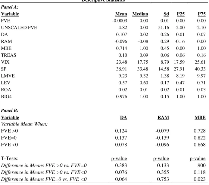
Panel A of Table 4 reports descriptive statistics. Unscaled realized and unrealized gains/losses on Level 3 instruments (UNSCALED FVE) is typically positive for non-financial services firms that hold Level 3 items. The mean of realized and unrealized gains/losses is a gain of approximately $4.8 million. Prior literature (e.g., Fiechter and Meyer 2009, Kolev 2009, Valencia 2011) does not directly report summary statistics of unscaled realized and unrealized gains/losses that are included in earnings. The dependent variable (FVE) used in the current study is realized and unrealized gains/losses on Level 3 instruments that are included in earnings, scaled by lagged total assets. Once scaled by lagged total assets, the mean of FVE is -.0003 and the median is 0.00 even though the mean of the unscaled variable is positive. This is due
COMPUSTAT reporting most financial statement data, including total assets, in millions. Firms with less than 1 million in total assets will have a decimal included in the denominator used for scaling.
The mean of level 3 holding gains and sales, scaled by market value of equity, reported by Kolev (2009) is -.039 and the median is 0.000. Valencia (2011) primarily focuses on