Rowing Blade Design using CFD

(1)

(2)

(3)

Rowing Blade Design using CFD

Master of Science Thesis

For obtaining the degree of Master of Science in Aerospace Engineering at Delft

University of Technology

M. Kamphorst B.Sc.

June 30, 2009

Faculty of Aerospace Engineering·Delft University of Technology

(4)

(5)

Preface

This report is a result of the research I did for my Master of Science Thesis as a conclusion of my studies at the faculty of Aerospace Engineering at Delft University of Technology. Last year has been a very eventful year in that I moved to Australia, got married to my wonderful wife Taryn and performed my graduation project. All of this would have been impossible without the help and support of many people, a number of whom I would like to mention.

Firstly I thank Dr. Michael Macrossan from the Center for Hypersonics at the University of Queensland in Brisbane, Australia, for inviting me to perform this very interesting research for him. Under his supervision I was allowed to grow and develop in insight and analysis of the problem given to me.

Secondly, I am Dr.ir. Bas van Oudheusden and Dr.ir. Leo Veldhuis grateful for their willingness to supervise this project from a different hemisphere. Their comments have been extremely valuable to me in improving the quality of my work. I would also like to thank Prof.dr.ir.drs. Hester Bijl for presiding my examination committee.

Wietse en Niels, thank you very much for helping me with writing this report and giving me advise on any matter with respect to my graduation.

Last but certainly not least I express my gratefulness and thanks to Taryn. Without her love, endurance and support I would not have been able do this.

It is my hope that the reader of this report will enjoy studying it and that the results of my work will contribute to the understanding of the physics of rowing.

Michiel Kamphorst ’t Harde, June 30, 2009

(6)

Abstract

How water and air flow around a rowing blade during a rowing stroke is poorly understood by the scientific community. Since important rowing races are won by time differences of only 0.4%, having a sound understanding of the flow will become more and more significant when it comes to rowing blade optimization. It is therefore the purpose of this Master Thesis project to investigate the flow around rowing blades using Computational Fluid Dynamics (CFD) in order to acquire enough knowledge and understanding of the flow to design a rowing blade.

Being limited by the options provided by the CFD software ANSYS CFX v.11.0, it is decided to do steady state simulations of a flat plate at the catch and the square-off of a rowing stroke. This way typical phenomena at both sides of the rowing spectrum varying from fully attached boundary layer to a completely separated boundary layer flow can be investigated. Using the Shear Stress Transport k-ωmodel to model the turbulence and the Volume of Fluid method in combination with a mesh adaption technique to capture the water-air interface, a numerical model is set up with an approximate error of 3.7% at the square-off and an estimated error of 1.5% at the catch.

The simulations of the flat plate at the square-off of the rowing stroke are compared to experi-ments performed by Caplan and Gardner (2007) [4][5] in order to validate the numerical model. It was found that when conducting scale model experiments to investigate rowing blade performance, it is important to establish what the minimum required towing tank dimensions are with respect to the dimensions of the scale model of the blade to be able to neglect blockage effects. When a flat plate is placed perpendicular to the flow, the depth of the towing tank is found to be required to be at least 4.5 times larger than the blade depth, whereas the required towing tank width is 4.3 times the blade width.

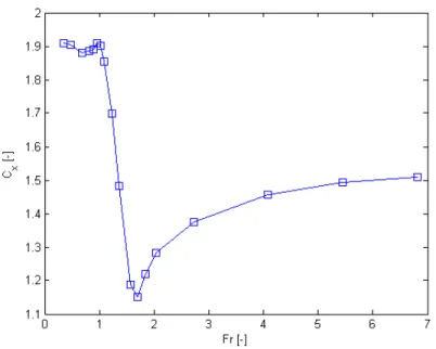
To obtain dynamic similarity when performing scale model experiments, one has to obtain the same Froude number and Reynolds number as would be obtained in a full scale experiment. For every part of the rowing stroke but in particular at the square-off, the magnitude of the Froude number is of major importance. When the Froude number at the square-off is close to unity, the blade force coefficients are highest, after which they drop to a minimum at the Froude number where a perfect hydraulic jump appears. This is usually at a Froude number of 1.25. At high supercritical Froude numbers, the force coefficients obtain an asymptotic value that will lie in between the two extrema described before.

(7)

For flow situations where the boundary layer is partially attached to the blade surface, the Reynolds number is important for the blade performance as well. Especially tangential forces are strongly influenced by the Reynolds number, whereas pressure dominated forces show only a very small increase when the Reynolds number is increased.

When designing a rowing blade, postponing boundary layer separation will increase the fluid mechanical efficiency of the blade during the early parts of the stroke. Delaying boundary layer separation can be achieved by rounding off the leading edge of the blade and by introducing a cam-ber that has a maximum that is not too close to either the leading or the trailing edge. Although introducing camber increases blade force coefficients, it directs the resultant blade forces away from the hull velocity vector and therefore decreases the fluid mechanical efficiency. When the higher blade force coefficients lead to the incorporation of a shorter shaft, the loss in efficiency can be balanced out.

After camber is introduced, the blade geometry can be adjusted such as to give the blade more surface area on the part of the leeward side pointing outward of the boat. This way, the inward pointing tangential force is reduced thus increasing efficiency at low oar angles. Although a rect-angular curved blade has a higher efficiency at the square-off, a compromise between a rectrect-angular blade and a blade where the bottom corner at the trailing edge is removed will yield a high overall efficiency during the rowing stroke.

If the proposed rowing blade designs are developed further, more optimization studies need to be performed with respect to the location and magnitude of maximum camber. Also the shape of the blade edges other than the leading edge as well as the blade planform shape need to be optimized. In addition to this, the shape of the part of the oar that connects the oar shaft to the rowing blade can be further designed as to improve efficiency at low angles of attack.

(8)

List of Figures

1.1 Sign convention for rowing . . . 4

1.2 Sign convention for simulations [21] . . . 5

1.3 Blade velocity variation during rowing stroke . . . 6

2.1 Oar angle according to Kleshnev [13] . . . 8

2.2 Velocities relative to water [21] . . . 8

2.3 Blade velocities relative to water [21] . . . 9

2.4 Force profiles for seat 1 and 7 during rowing stroke at a rate of 40.8 min−1 _{. . . . .} ₁₁

2.5 Mean efficiency, mean propulsion power, shape factor, center of force and maximum force displayed for different seats [23] . . . 11

2.6 Hull kinematics for stroke rate = 40.8 min−1 _{. . . .} ₁₂

2.7 Data for stroke rate = 40.8 min−1 _{. . . .} ₁₃

3.1 Setup of Caplan and Gardners’ experiments [4] . . . 15

3.2 Projected areas for the model oar blades tested [4] . . . 16

3.3 Projected areas for the model oar blades tested [5] . . . 16

3.4 Force coefficients compared for flat and curved rectangular blade [4] . . . 16

3.5 Caplan and Gardner results for rectangular flat plate . . . 17

3.6 Domain layout for simulations by Coppel (2008) [3] . . . 17

3.7 Drag coefficientCD vs. angle of attackα[3] . . . 18

4.1 Macon shape and dimensions of the tulip-shaped blade [8] . . . 19

4.2 Big Blade shape and dimensions [8] . . . 20

4.3 Smoothie2 Vortex Blade shape and dimensions [8] . . . 20

4.4 Fat Blade shape and dimensions [8] . . . 21

4.5 Slik Blade [26] . . . 21

4.6 Force coefficients compared for flat and curved Big Blade [4] . . . 22

4.7 Kinematics at initial phase of stroke [4] . . . 22

4.8 Force coefficients for different curvatures applied to rectangular blade [4] . . . 23

4.9 Comparison between curved Big Blade and curved rectangular blade [4] . . . 23

4.10 Vortex Edge [27] . . . 24

(11)

6.2 Flat plate . . . 34

6.3 Plate and symmetry plane mesh after mesh refinement . . . 35

6.4 Force coefficient in flow directionCX for various mesh sizes . . . 36

6.5 Force coefficient perpendicular to flow directionCY for various mesh sizes . . . 36

6.6 Vertical force coefficientCZ for various mesh sizes . . . 37

6.7 Volume fraction Φ and symmetry plane mesh after mesh refinement . . . 38

6.8 Domain length (x) vs. force coefficient in flow directionCX . . . 38

6.9 Domain length (x) vs. vertical force coefficientCZ . . . 39

6.10 Water surface for domain length = 500 mm . . . 40

6.11 Water surface for domain length = 800 mm . . . 40

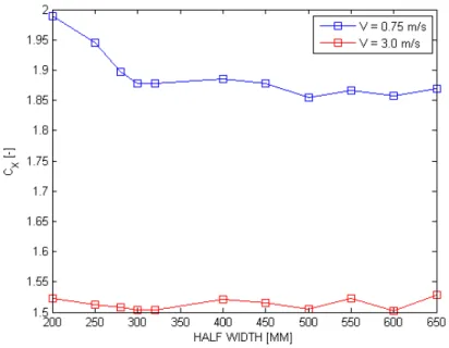
6.12 Force coefficient in flow direction CX for varying domain half widths . . . 41

6.13 Vertical force coefficientCZ for varying domain half widths . . . 41

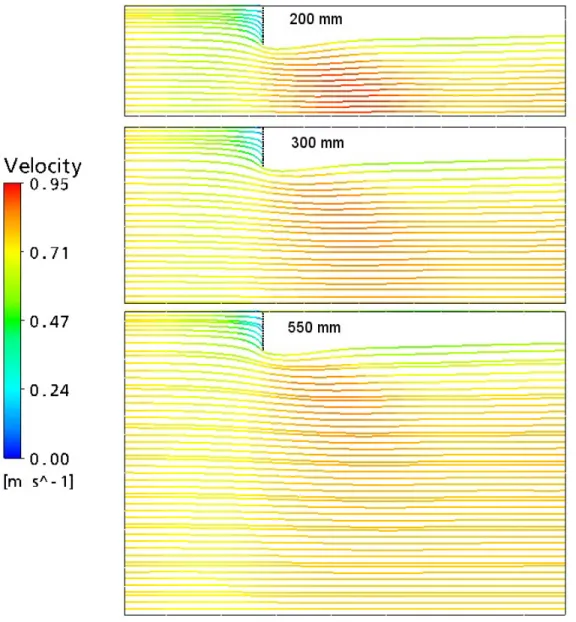
6.14 Flow development for various domain half widths at 30 mm depth. Top view of horizontal plane . . . 42

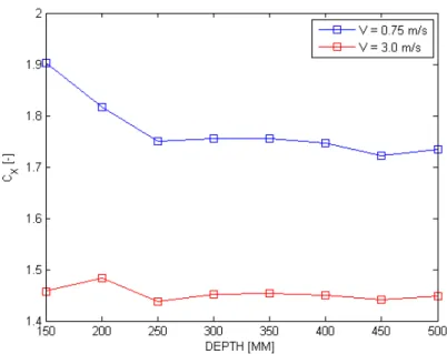
6.15 Force coefficient in flow direction CX for varying domain depth . . . 43

6.16 Vertical force coefficientCZ for varying domain depth . . . 43

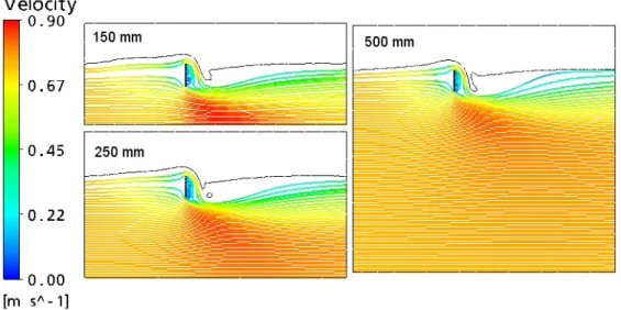
6.17 Flow development for various domain depths in the symmetry plane . . . 44

6.18 Froude numberF r vs. force coefficient in flow directionCX, constant water density and viscosity, quarter scale flat plate . . . 45

6.19 Froude numberF rvs. force coefficient perpendicular to flow directionCY, constant water density and viscosity, quarter scale flat plate . . . 45

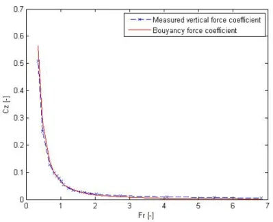
6.20 Froude number F r vs. vertical force coefficient CZ, constant water density and viscosity, quarter scale flat plate . . . 46

6.21 Froude numberF r vs force coefficient in flow directionCX, full scale flat plate . . . 47

6.22 Froude numberF r vs. force coefficient perpendicular to flow directionCY, full scale flat plate . . . 47

6.23 Froude numberF r vs vertical force coefficientCZ, full scale flat plate . . . 48

6.24 Flow behaviour at various Froude numbers, side view . . . 48

6.25 Force coefficient in flow direction CX as a function of the inlet turbulence intensity, quarter scale flat plate . . . 49

6.26 Force coefficient in flow direction CX as a function of the inlet eddy length scale, quarter scale flat plate . . . 49

6.27 Reynolds number dependence for flat plate . . . 50

6.28 Force coefficient in flow direction CX dependence on Reynolds and Froude number for full scale flat plate . . . 50

6.29 Vertical force coefficientCZ dependence on the Reynolds and Froude number for full scale flat plate . . . 51

7.1 Flat plate dimensions . . . 53

7.2 Mesh close to flat plate . . . 53

7.3 Influence of number of mesh cells on flat plate forces . . . 54

7.4 Influence of maximum cell size on flat plate forces . . . 55

7.5 Influence of domain dimensions on normalized normal force on the blade . . . 56

7.6 Definitions of domain dimensions . . . 57

7.7 Water surface . . . 58

7.8 Velocity contour at a depth of 110 mm . . . 59

7.9 A close-up of the velocity contour at a depth of 110 mm . . . 59

7.10 Streamlines around the leading edge at a depth of 110 mm . . . 60

7.11 Separation bubble on windward side . . . 60

(12)

7.13 Pressure coefficient at a depth of 110 mm . . . 62

7.14 Streamlines around the trailing edge at a depth of 110 mm . . . 62

7.15 Locations of boundary layer profiles . . . 63

7.16 Boundary layer profiles for leeward side at 110 mm depth . . . 64

7.17 Boundary layer profiles for windward side at 110 mm depth . . . 65

7.18 Influence of the Froude number on flat plate forces . . . 65

7.19 Pressure coefficient CP distribution along the chord of the flat plate . . . 66

7.20 Water surface for various Froude numbers . . . 67

7.21 Contribution of pressure and viscous forces to tangential force coefficientCT . . . . 68

7.22 Relation between ratio of tangential over normal forces and Froude number . . . 68

7.23 Separation bubble for various Froude numbers . . . 69

7.24 Separation bubble for various Froude numbers . . . 70

7.25 Influence of the Reynolds number on flat plate force coefficients . . . 70

7.26 Pressure coefficient for various Reynolds numbers . . . 71

7.27 Contribution of pressure and viscous forces toCT . . . 71

7.28 Wall shear stress for various Reynolds numbers . . . 72

7.29 Separation region for various Reynolds numbers . . . 72

7.30 Surface area exposed to air for variousRe . . . 73

7.31 Boundary layer development for various Reynolds numbers . . . 74

7.32 Development of production term with increasing Reynolds number . . . 74

7.33 Development of pressure gradient with increasing Reynolds number . . . 75

7.34 Relation between viscous wall shear stress and Reynolds number . . . 75

7.35 Relation between viscous dissipation and Reynolds number . . . 76

8.1 Configuration of the rowing blade . . . 78

8.2 Configuration of the rowing blade . . . 78

8.3 Surface mesh of the oar configuration . . . 79

8.4 Surface mesh on the leading edge . . . 79

8.5 Outer mesh . . . 80

8.6 Outer mesh around the leading edge . . . 80

8.7 Blade performance as a function of aspect ratio . . . 82

8.8 various leading edge shapes . . . 83

8.9 Streamlines for rounded leading edge . . . 84

8.10 Streamlines for leading edge with lower corner tapered . . . 85

8.11 Blade performance as a function of location of maximum camber . . . 86

8.12 Streamlines for varying location of maximum camber . . . 87

8.13 Blade performance as a function of magnitude of maximum camber . . . 88

8.14 Layout of the quintagonal rowing blade . . . 89

8.15 Layout of the triangular rowing blade . . . 89

8.16 Water surface at angle of attackα= 90o for rectangular blade . . . 90

8.17 Water surface at angle of attackα= 90o for quintagonal blade . . . 91

8.18 Water surface at angle of attackα= 90o for triangular blade . . . 91

8.19 Water surface at angle of attackα= 10o for rectangular blade . . . 92

8.20 Water surface at angle of attackα= 10o _{for quintagonal blade . . . .} ₉₂

8.21 Water surface at angle of attackα= 10o _{for triangular blade . . . .} ₉₃

8.22 Geometry variation during next design iteration . . . 93 8.23 Fluid mechanical efficiency of rowing blade during Dr. Kleshnev’s experiments [21] . 94

(13)

List of Tables

7.1 Domain size . . . 57

8.1 Parameter values for fluid mechanical efficiency . . . 81

8.2 Blade performance at catch for various leading edge shapes atα= 10o . . . 84

8.3 Blade performance for various blade geometriesα= 90o _{. . . .} ₉₀

8.4 Blade performance for various blade geometries atα= 10o _{. . . .} ₉₁

8.5 Ranking of the three different blade geometries at catch and square-off . . . 92

8.6 Comparison of rectangular and quintagonal blade to ’Big Blade’ . . . 93

B.1 simulation settings (1/2) . . . 104

(14)

List of Symbols

English Symbols

Bn normal blade force [N]

Bt tangential blade force [-]

CN normal force coefficient [-]

CP pressure coefficient [-]

CT tangential force coefficient [-]

CX,CY,CZ force coefficients in Cartesian directions [-]

D blade depth [mm]

˙

Eblade flux of blade energy loss to water [J/s] ˙

Ein energy flux put into oar by rower [J/s]

F r Froude number [-]

G source term [m2_]

H height [m]

L length [m]

M order of series expansion [-]

N number of mesh cells [-]

Ph handle power [J/s]

Pp propulsive power [J/s]

Pwb waste power [J/s]

Pws waste power due to hull fluctuations [J/s]

Re Reynolds number [-]

S blade surface area [-]

S shape factor [-]

Sij strain rate tensor [s−1]

T torque [Nm]

V velocity [m/s]

W width [m]

(15)

c blade chord length [m]

c1,C2 empirical constants [-]

eb Kleshnev blade efficiency [-]

eN percentage error in normal force [-]

eres percentage error in resultant force [-]

eT percentage error in tangential force [-]

es effectiveness of boat hull propulsion [-]

f variable for Richardson Extrapolation [-]

fs propulsive effectiveness for hull propulsion [-]

gk independent scalar [-]

h mesh cell edge length [m]

lm mixing length [m]

k kinetic energy of turbulence [J]

r location vector of rowing blade [m]

ti inflation layer thickness [m]

x, y, z Cartesian coordinates for position [m]

xCoP Location of center of pressure along chord line [m]

ui,j,k velocity in Cartesian directions [m/s]

u0_i,j,k turbulent velocity fluctuation in Cartesian directions [m/s]

x/c blade chord fraction [-]

Greek Symbols

α blade angle of attack [deg]

δij Kronecker delta [-]

turbulent dissipation [J/s]

η fluid mechanical efficiency [-]

µ dynamic viscosity [Pa s]

ν kinematic viscosity [m2 _s−1_]

νt eddy viscosity [m2 _s−1_]

ρ density [kg/m3]

Π tangential force to normal force ratio [-]

τij viscous stresses [N s m−1]

τ_ijR Reynolds stresses [N s m−1]

Φ volume fraction [-]

φ oar angle [deg]

ψ oar angle in horizontal plane [deg]

ψcof weighted average oar angle [deg]

ω oar angular velocity, [deg/s]

(16)

CHAPTER

1

Introduction

1.1

Background

Rowing is a form of propulsion on water that has been used throughout the course of history. From the impressive Phoenician triremes in ancient times to the 2008 Olympic games in Beijing, rowing is a form of propulsion that survived the ages into modern times. But although human kind has known the concept of rowing for several millenniums, the fundamental flow behaviour around a rowing blade has never been fully understood.

In recent history, only a few scientists are known to have attempted to perform experiments with rowing blades. Dr. V.I. Kleshnev from the Australian Institute of Sport has measured oar bending during a rowing stroke, whereas Dr. N. Caplan and Dr. T.N. Gardner have measured rowing blade forces in a water flume. Although these experiments give an idea of the performance of rowing blades throughout a rowing stroke, the behaviour of the water and air flow and the dependence of the blade performance on various factors such as water depth, Froude number and Reynolds number are are still ill understood.

The development of Computational Fluid Dynamics (CFD) software and fast computersystems has now made it possible to compute and visualize fluid flows. Although this has been applied in many area’s of engineering and science, the combination of moving meshes and interface capturing has made the accurate simulating of a rowing blade during the rowing stroke a challenging project. Considering the narrow margins with which rowing races are won nowadays, CFD will become increasingly important in designing new rowing blades. During the Men’s eight rowing final in the 2008 Beijing Olympic games, the difference between the number one and number two on the finish line of the 2000 m was 1.22 seconds. Assuming the hull speed at the finish was 7 m/s, this means that the Canadian and the Great Britain teams finished with a 8.5 m difference. On a 2000 m race, this is a difference of 0.4%. Narrow margins like this signify the importance of capabilities of optimizing rowing blade design.

(17)

model the flow around a rowing blade, investigate the dependence of the blade performance on several parameters and use this knowledge to design a rowing blade.

1.2

Problem statement

The goal of this Master Thesis research can be defined as:

Use a commercial CFD package to investigate the flow around a rowing blade, in particular the effects of the Froude number and the Reynolds number on the rowing blade forces. Use the results to design a rowing blade

To accomplish this goal, the commercial CFD package ANSYS CFX v.11.0 is used to simulate the fluid flow around a rowing blade at several stages of the rowing stroke. Because the current version of ANSYS CFX is not capable of using mesh refinement in transient simulations and be-cause its capabilities for mesh deformation are limited, the choice has been made to do steady state simulations.

1.3

Objectives

As stated above, it is the purpose of this Master Thesis project to investigate the water and air flow around a rowing blade. This is done using CFD. As with any computational method, the CFD model that is used will have to be tested against experiments. The experiments that will be used as reference material are the tests performed by N. Caplan and T.N. Gardner [4] [5], a more detailed description of which will follow in chapter 3.

After the numerical model is validated, it can be used to investigate water and air flow around the blade. Often when tests are performed on rowing blades, the size of the blades is limited by the dimensions of the towing tank that is available. Since this results in the use of scale models of rowing blades, it is important to obtain dynamic similarity with the full scale flow. As chapter 3 will show, not all scientists are fully aware of this. Therefore it is the purpose of a part of this report to investigate the effects of the two similarity parameters the Froude number and the Reynolds number on the rowing blade performance.

Once the effects of the Froude number and the Reynolds number on the blade forces are estab-lished, the rowing blade performance can be investigated for various typical flow situations. Using a rectangular flat plate to model a rowing blade, knowledge is accrued about various flow features that appear. This knowledge can then be used to start the conceptual design of a rowing blade.

Summarizing, the objectives of this Master Thesis project can be stated as follows: 1. use existing experimental results to validate the results of the numerical model 2. investigate the influence of the Froude number on the blade forces

3. investigate the influence of the Reynolds number on the blade forces

4. analyze the water and air flow around a flat rectangular blade at different stages during the rowing stroke

(18)

1.4

Requirements

For each rowing team it will depend upon the configuration of the boat what sort of rowing blade is chosen. Children teams for example will use rowing blades that are easier and lighter to handle than adult teams. For this Master Thesis research it is decided to design a blade for a Men’s Eight rowing team that uses sweeping blades, i.e. each rower operates only one oar. Sweeping blades generally have a frontal surface area of 0.125 m2

Rowing Australia, the rowing authority in Australia, has posed requirements on the geometry of rowing boats and rowing oars in ’Rowing Australia rules of racing and related by-laws’ [29]. With respect to sweeping blades, Rowing Australia’s safety requirements state that each blade must have a minimum thickness of 5 mm at a distance of 3 mm from the edge. This is the only requirement that Rowing Australia poses on the geometry of the rowing blade. In addition to this, a visit to the local rowing club resulted in the conclusions that oar shafts generally have a thickness of 45 mm and are placed at an angle of 160o _{with respect to the blade’s top edge.}

To be able to assume a rigid rowing blade, sufficient stiffness has to be provided. Most rowing blades used in competitive rowing are made from laminated timber or a composite material based on laminated timber and carbon fibre. The combination of blade curvature, the chosen material and the connection part between the oar shaft and the blade make the blade sufficiently rigid when its thickness is equal to the required minimum thickness of 5 mm.

Since it is the aim of this Master Thesis to design a rowing blade that could be used in com-petition, the rowing blade that will be designed has to have an efficiency that is equal to or better then the efficiency of existing rowing blades. As a reference the performance of a ’Big Blade’ as used in experiments performed by Dr. V.I. Kleshev, will be used.

The requirements posed to the design can be summarized as follows: • Geometry

1. minimum blade thickness: 5 mm at 3 mm distance from blade edge 2. blade frontal surface areaS = 0.125 m2

3. oar shaft diameter: 45 mm

4. angle between oar shaft and blade top edge: 160o • Structural

1. provide blade with place for shaft attachement

2. provide sufficient blade thickness for structural stiffness • Performance

1. the designed rowing blade should be at least as efficient as existing rowing blades

1.5

Definitions and rowing terminology

Since the technicalities of rowing may be new to most of the readers of this report, a list of rowing terms used in this report is given below.

(19)

• sweeping - type of rowing where the rowers use both hands to move one oar. Average blade size is big.

• sculling - type of rowing where each rower operates two oars, one with each hand. Average blade size is small

• rowing blade - the large surface area part at the end of the oar that moves through the water, thus propelling the boat

• shaft - the timber, carbon fiber or fiber glass boom connecting the handle and the blade • handle - the part of the oar the rower exerts force on through his hands

• hull - the outer shell of the rowing boat that is in contact with the water

• catch - phase of stroke when blade enters the water and a torque is applied to the handle • square-off - phase of stroke when oar is at an angle of 90o _{with respect to the hull centerline}

in the horizontal plane

• release - phase of stroke when oar is pulled out of the water • gate - pivot point of the oar

Figure 1.1 shows the angles and velocities that will be used throughout this report. The oar angleψis the angle between the symmetry axis of the rowing boat hull and the oar in the horizontal plane. The angular velocity of the oar is defined as ω = ˙ψ. Adding the velocity of the hullVhull to the angular velocity of the oar at the position of the rowing bladerresults in the blade velocity Vblade relative to the water (equation 1.1). Angle of attackαis the angle betweenVblade orVb and the oar axis.

Vblade =Vhull+ω×r (1.1)

Figure 1.1: Sign convention for rowing

Taking the rowing blade as reference, figure 1.2 shows the relative velocities and angles for the simulations. In this figure, Bn and Bt are the normal and tangential force respectively. The tan-gential force direction is defined away from the boat.

(20)

Figure 1.2: Sign convention for simulations [21]

Howαrelates toψis shown in figure 1.3 (a). Figure 1.3 (b) shows the resulting blade velocity for the angle of attack. The data for these figures has been provided by Dr. V.I. Kleshev, who measured oar angles, handle forces and hull speeds for a men’s eight rowing at a stroke rate of 40 strokes/min. From these figures it can be deduced that at the catch, whereψ = 37o_,_α_{= 10}o _with a correspondingVb = 4.7 m/s, whereas at the square-off, bothαandψare 90o_and _Vb _{= 1.4 m/s.}

The forces on a rowing blade depend on three categories of properties that are listed below: • fluid properties - density, viscosity

• flow properties - freestream velocity, plate depth

• geometrical properties - plate size and orientation, water depth and distance from hull and bank

To be able to compare the performance of different blades, these properties need to be non-dimensionalized in a logical manner. Assuming constant geometrical properties, the blade forces will depend on both the fluid and flow properties. The four parameters belonging to these categories can be captured by two non-dimensional parameters: the Reynolds number Re and the Froude number F r. In this report, the effect of these two non-dimensional parameters on the normal and tangential force coefficients (CN and CT) will be investigated. These non-dimensionalized parameters are defined as:

Re=ρV D µ (1.2) F r=√V gD (1.3) CN = Bn 1/2ρV2_S (1.4) CT = Bt 1/2ρV2_S (1.5)

Whereρis the water density (usually with a value of 997 kg m−3),gthe gravitational acceleration (9.81 m s−2), S the blade surface area (0.125 m2). In case of a curved blade, this surface area is defined as the projection of the rowing blade upon a plane that touches the four corners of the windward side of the rowing blade. µis the water dynamic viscosity (8.899 ×10−4 _{Pa s),}_D _{is the}

(21)

(a) Oar angle vs. angle of attack (b) Angle of attack vs. blade speed

Figure 1.3: Blade velocity variation during rowing stroke

1.6

Report structure

Because rowing is such an old and widespread activity, there exist numerous views on how to row as efficient as possible. Chapter 2 will therefore give an overview of scientific approaches towards defining rowing efficiency. Then in chapter 3, the work of a number of scientists on the analysis of the performance of rowing blades will be discussed, followed by an overview of modern rowing blade designs in chapter 4. To be able to set up a computational method, in chapter 5 the methods to model the turbulence and to capture the water-air interface are discussed. Chapter 6 then starts with the analysis of the flow around a flat plate at square-off, followed by an analysis of flat plate performance at the catch of the rowing stroke (chapter 7). The accrued knowledge will then be used to design a rowing blade in chapter 8, after which this report is concluded with chapters 9 and 10.

(22)

CHAPTER

2

The efficiency of rowing

During the last few years a lot of effort has been put into finding a solid theoretical basis for rowing. Rowing myths have been revealed and created and a unified scientific model seems to be a mere dream. This chapter is dedicated to the ideas and work with respect to rowing efficiency of two players in this field: Dr. V.I. Kleshnev and Dr. M.N. Macrossan. In the first section the focus will be on fluid mechanical efficiency, while the second section will take into account the broader perspective of rower and boat. Section 2.3 will conclude with a discussion on how to proceed in the course of the current research.

2.1

Fluid mechanical efficiency

Looking purely at the fluid mechanical efficiency of rowing blades, there are several interpretations available throughout the scientific community of what that exactly means. In two of his reports, which basically cover the same material but to different extents, Dr. V.I. Kleshnev [13] [14] uses the following definition for oar blade efficiency,eb:

eb ≡Pp

Ph (2.1)

wherePhis the handle power, which is the power exhibited at the handle of the rowing oar. The propulsive powerPpis defined as the difference between the handle power and the waste power due to blade movement through the water,Pwb. This waste power is the product of the normal force on the oar blade (Fb) and the velocity of the blade projected unto the direction of the hull centerline, or written in mathematical form: Pwb =Fbvbcosφ, with φ the angle between the normal to the hull velocity direction and the oar shaft longitudinal axis, as shown in figure 2.1 as taken from [22], whereφ=θc

In the performed experiments to which both reports refer, forces and speeds were measured for several seating configurations, boat speeds and rowing rates. The blade efficiencies for the

(23)

Figure 2.1: Oar angle according to Kleshnev [13]

different situations are all within a range of 72% to 96% with an average of 80–83%. Kleshnev con-cludes that improvement of the blade efficiency can increase the overall rowing efficiency with 3–5%. Based on the work of Dr. M.N. Macrossan, a different approach towards oar blade efficiency can be taken. Firstly, Macrossan shows how the myth of back-splash acts against both intuition and physics [22]. In professional rowing, rowers are often instructed by their coaches to lower their blade into the water just before the blade is at its furthest rearward point. What happens then is that water is splashed in hull velocity, thus exerting a force on the blade opposite hull velocity, which in turn helps the rower to start the rowing stroke with a higher initial angular momentum. It is easily understood that by exerting a force on the rowing blade opposite to the direction of hull speed, the hull velocity is reduced, thus reducing the overall rowing efficiency.

Figure 2.2: Velocities relative to water [21]

In addition to this, one can look at the energy efficiency of the rowing blade whilst in the water during a propulsive rowing stroke between catch and square-off. Using the definitions provided in figures 2.2 and 2.3, the energy the blade exchanges with the water ˙Eblade can be defined as follows:

(24)

Figure 2.3: Blade velocities relative to water [21]

˙

Eblade=Bnvs−Btvp (2.2) with vs the slipping velocity component andvp the sliding, parallel velocity component. Both velocity components are defined as:

vs=−Vhullsinψ+ωl (2.3)

vp=Vhullcosψ (2.4)

In these equations,Vhullis the hull velocity andlthe distance between the gate and the rowing blade center of pressure.

The energy the rower puts into the oar ˙Einis defined as: ˙

Ein=T ω (2.5)

withT the torque the rower applies to the oar and ωthe angular velocity of the oar. Knowing this, the fluid mechanical efficiency of the rowing blade can be calculated as:

η= ˙

Ein−Eblade˙ ˙

Ein (2.6)

Combining equations 2.2 through to 2.6, the fluid mechanical efficiency of the blade is:

η= Vhull ωl sinψ+ Bt Bncosψ (2.7) During the first part of the rowing stroke,Btwill be negative. Therefore, a tangential to normal force ratio Π can be defined as

Π =−Bt

Bn (2.8)

Π is an indication of the direction of the resultant force with respect to the hull velocity. At oar angles smaller than 90o _{a low Π means that the angle between the hull velocity vector and} the resultant blade force vector is smaller thus increasing fluid mechanical effiency. Substituting equation 8.2 into equation 2.7, the fluid mechanical efficiency of the rowing blade is calculated as:

η=Vhull

(25)

2.2

Biomechanical efficiency

Increasing the efficiency of rowing depends on more than just increasing blade efficiency. In one of his earliest reports on the subject, Kleshnev takes into account the efficiency of the hull (which he calls shell).

In Kleshnev (1998) [13], the overall efficiency is defined as the sum of the blade efficiency and the shell velocity efficiency. The shell velocity efficiency results from velocity fluctuations of the hull and the resulting loss of energy. Kleshnev concludes that the overall energy loss of 22.4% is due to water movement around the blade (17.8%) and shell velocity fluctuations (5.6%) It appears that improving the blade efficiency can have a large positive influence on the overall rowing efficiency. This is underlined by [14], where Kleshnev states that the (undefined) rowing effectiveness can be increased by 8.2%, of which 6.4% comes from blade efficiency improvements and 1.8% from hull velocity fluctuations.

In his 1999 report, Kleshnev [14] defines a large series of parameters. First of all, there is waste energy due to shell velocity fluctuations, Pws, which is calculated as: Ews = P_kv3

i −kv3, with v the average shell velocity during the stroke. Then there is the propulsive effectiveness for shell propulsion,fs= Vreal Vmax = _esP p/k Pp/k 1/3

=es1/3= effectiveness of boat shell propulsion.

Kleshnev concludes in his report that reducing the drive time to stroke time ratio will increase the effectiveness of boat shell propulsion. He also states that an increased stroke rate will increase the shell velocity fluctuations, thus decreasinges.

In addition to this there are two more reports from Kleshnev, one [15] of which shows the re-sults of measuring the power produced by different parts of the human body. The legs prove to provide 45% of the rowing power, the trunk 32% and the arms account for the remaining 23%. This results in the fact that 53% of the power is provided at the oar handle, while 47% is applied at the footstretcher. Secondly, [16] states that the best results in rowing races will be obtained when a flat force profile is created by accelerating the body as fast as possible. These conclusions are elaborated upon by Macrossan in M.N Macrossan and N.W. Macrossan (2008) [23].

In his report, Macrossan uses Kleshnev’s data to investigate the influences of blade efficiency, force profile and force magnitude on the rowing performance of an elite eight rowing at the Aus-tralian Institute of Sport. There is a number of parameters Macrossan incorporates in his research. Firstly there is the force profile, that is described by the shape factor (S). The shape factor is defined asS≡ B

Bmax and varies from 0 to 1. A shape factor close to 1 indicates a flat force profile.

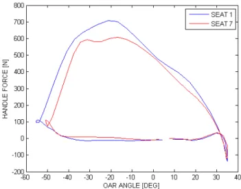
When at the catch the maximum force is reached sooner and kept constant throughout the stroke, a rectangular force profile is developed, resulting in a shape factor close to one. Two examples of a force profile are shown in figure 2.4. As seen before, Kleshnev seems to be in favour of a shape factor close to unity.

To be able to say something about how the forces are applied over the stroke, Macrossan defines the:

“weighted average oar angle where the weighting is proportional to the force developed.” This variable ψcof can be calculated as ψcof = Bnψ

Bn

. It indicates at which oar angle half of the integrated force is applied, therefore it is a measure of when most of the force is applied: near catch

(26)

Figure 2.4: Force profiles for seat 1 and 7 during rowing stroke at a rate of 40.8 min−1

or near square-off.

Finally there is the average propulsion power, ˙Ep≡Eprop˙ =BnsinψV and the mean efficiency η. For a mean hull speedV = 5.19m/sand a stroke rate of 21.1 min−1, values for the different variables are given in Figure 2.5, taken from [23].

Figure 2.5: Mean efficiency, mean propulsion power, shape factor, center of force and maximum force displayed for different seats [23]

Because of the many factors involved, no clear conclusion can be drawn on what to do to win a rowing race. Based on his findings, Macrossan suggests that applying a greater force near square-off might increase blade efficiency. This is based on the idea that although efficiency is high at the beginning of the stroke, the blade force is very low and angled away from the hull velocity vector. Because of the increased directional efficiency near square-off, it can be worthwhile investigating the idea of shorter strokes at higher rates. This opposes Kleshnev’s claim of better rowing efficiency by applying higher forces close to the catch of the stroke.

(27)

(a) Hull velocity vs. oar angleψ (b) Hull acceleration vs. oar angleψ

Figure 2.6: Hull kinematics for stroke rate = 40.8 min−1

2.3

Optimizing the fluid mechanical efficiency of the rowing

blade

Estimating and optimizing rowing performance is a process that involves a large number of variables. The fluid mechanical efficiency of the blade, the stroke rate, the shape factor and the magnitude of the shell velocity fluctuations each individually have to be optimized according to the wishes of the rowing team. For a rowing blade designer it is important to design a blade such that its fluid mechanical efficiency is as high as possible. Looking back at the equation for the fluid mechanical efficiency of the blade (8.1), every variable has to be taken into account to achieve a high efficiency. Firstly, the hull velocity, Vhull, is to be kept as high as possible. Figures 2.6 (a) and (b) are obtained using measurements performed with a Men’s Eight rowing team. The oar angle ψ de-picted in these figures is the mean value of the oar angles for the eight seat positions at a particular moment in time. These figures show how the fluid mechanical efficiency has potential for increase just after the catch and for 55o_≤_ψ_≤₈₀o_{as well as just before release.}

Secondly,landω need to be kept as small as possible. Whilstlwill be constant for a particular oar shaft,ω depends on the stroke rate of the rowing team. Figure 2.7 (a) shows, lowω requires a small handle force, i.e. fluid mechanical efficiency will be increased when the blade forces are small. Figure 2.7 (b) indicates that a lowωcorresponds to the phase of the stroke just after the catch and before release.

Thirdly and finally, the parameter that will be of main interest for this research is force ratio Π. Π will strongly depend on the rowing blade design and has to be kept as small as possible to achieve optimal fluid mechanical efficiency. In other words, the inward pointing tangential force has to be as small as possible with respect to the normal force to increase fluid mechanical efficiency. In chapter 8, the influence of blade design on this factor Π will be demonstrated.

(28)

(a) Normalized handle force vs. oar angular velocityω (b) oar angular velocityω vs. oar angleψ

(29)

CHAPTER

3

Reference experiments

When a numerical model is developed, it is important to test it and compare the results to experi-ments performed by others. These experiexperi-ments can be both empirical and numerical. This chapter gives an overview of relevant experiments that have been done in the area of the current research and that can be used to validate the numerical model that is to be developed during the course of this project. Section 3.1 will describe the empirical experiments, while section 3.2 reports the results of numerical experiments.

3.1

Caplan and Gardner

In Caplan and Gardner (2007) [4][5] Nicholas Caplan and Trevor Gardner measured forces on a flat plate and several rowing blades in a water flume experiment. Because of the dimensional limitations of their flume, they used quarter scale blades. Not realizing that the Froude number could be of any importance, they tried to realize dynamic similarity by investigating the effects of Reynolds number, but took no account of the Froude number variation between model and experiments. The flume was limited to a water velocity of 0.85 m/s, but they concluded that for velocities higher than 0.7 m/s the Reynolds number had no influence on the experimental results. Therefore they performed the experiments at 0.75 m/s.

Figure 4.7 shows experimental setup and the forces and definitions used in the papers. The pro-jected areas of the used blades are depicted in Figures 3.2 and 3.3. Figure 3.4 shows their results for a flat and curved rectangular blade.

To get an estimation of the quality of Caplan and Gardners’ experiments, their force coefficients for the rectangular flat plate are transformed from lift and drag components into normal and tan-gential components. This is depicted in figures 3.5 (a) and (b).

The tangential force component can be expected to change sign when the angle of attack in-creases from α≤90o _to _α_≥₉₀o_{. Caplan and Gardners’ results show a positive tangential force} component for every angle of attack. ThisCT has an average value of 0.0366 and a standard de-viation of 0.0182. It can be concluded therefore that the experimental setup Caplan and Gardner

(30)

Figure 3.1: Setup of Caplan and Gardners’ experiments [4]

used is not able to detect tangential forces, i.e. forces parallel to the oar shaft axis. This is an interesting conclusion, since they do use a strain gauge for this direction, namely strain gauge V in figure 4.7. Thus, assuming all their strain gauges have the same characteristics, it can be concluded that the magnitude of tangential forces is smaller than the error in the force measurements. This means that the error in the calculated force coefficient is larger than 0.037. The measured CN for

(31)

Figure 3.2: Projected areas for the model oar blades tested [4]

Figure 3.3: Projected areas for the model oar blades tested [5]

Figure 3.4: Force coefficients compared for flat and curved rectangular blade [4]

α= 90o _{is 1.95. This value can be used as a reference value when investigating the flow around a} flat plate at square-off in chapter 6.

3.2

Coppel

In an attempt to numerically investigate the flow around a rowing blade, Coppel et al. (2008) [3] used Fluent to model this flow. Instead of using a free surface, the air-water interface was modeled using a symmetry plane as is shown in figure 3.6. Two turbulence models (k- and SST k-ω) are tested together with a first and a second order upwind scheme. The calculated drag coefficients are

(32)

(a) Normal force coefficientCN vs. (b) Tangential force coefficientCT vs. angle of attackα angle of attackα

Figure 3.5: Caplan and Gardner results for rectangular flat plate

compared to the empirical results obtained by Caplan and Gardner (2007) [4]. The resulting graph is depicted in figure 3.7.

This graph implies that SST k-ω performs better in these type of experiments than the k-model. Care needs to be taken though since the free surface has not been taken into account while its influence is expected to be significant. Coppel et al. conclude that the Reynolds number assumption of Caplan and Gardner [4] is incorrect. For a Macon blade atα= 90o_{, they measure a} CDof 1.97 at an inlet velocity of 0.75 m/s. For inlet velocities of 2.5 m/s and 5 m/s, the measured CDis 1.67. This is interpreted as a Reynolds number effect whilst it may well be a Froude number effect in as far as the latter is allowed for by a numerical model that does not include air flows and models the water-air interface with a symmetry plane.

(33)

(34)

CHAPTER

4

Current rowing blade designs

Designing a rowing oar blade is not a unique phenomenon in history; many have gone before us and many will follow. Section 4.1 gives an overview of the mainstream blade designs. The designs described in this section are produced by Concept2, a company specialized in rowing materials and equipment. An introduction into the various features used in modern rowing blade design is given in section 4.2.

4.1

Modern blade designs

A traditional rowing blade used for over thirty years is the tulip-shaped Macon blade. Figure 4.1 shows the main features of this blade.

Figure 4.1: Macon shape and dimensions of the tulip-shaped blade [8]

During the last decade a lot of improvement has been made in the area of rowing blade design. Firstly, there is the Big Blade. The Big Blade is designed to displace a large amount of water during the square-off and the last part of the stroke. Shape and dimensions of this blade are shown in Figure 4.2. The wide outboard edge of this blade produces an increased amount of leverage at

(35)

square-off, thus providing the rower with the option of using a shorter shaft.

Figure 4.2: Big Blade shape and dimensions [8]

Secondly, there is the Smoothie2 Vortex Blade. The philosophy behind this blade is that a turbulent flow at the low pressure side of the blade, created by the so called vortex edge, during the initial part of the stroke just after catch, provides more water grip. For rowers who prefer to use most of their power during the first part of the stroke, this blade will prove very convenient. The shape and dimensions of this blade are depicted in Figure 4.3.

Figure 4.3: Smoothie2 Vortex Blade shape and dimensions [8]

Concept2’s most recent design is the Fat2 Blade. This blade provides the rower with an even heavier load at the first phase of the stroke. After the last phase of the stroke the blade is designed to create less energy dissipation. An overview of the blade’s characteristics is given in Figure 4.4.

(36)

Figure 4.4: Fat Blade shape and dimensions [8]

A different approach to blade design has been taken by Croker Oars with their Slik Blade (Figure 4.5). The Slik Blade relies on as little splashing at catch and release as possible and is visibly not designed to create extra turbulence.

Figure 4.5: Slik Blade [26]

4.2

Design features

Other than defining the cross-sectional shape, one of the main features to optimize the design is to change the curvature of the blade. As the static experiments of Figures 4.6 and 3.4 show, adding curvature to a flat blade increases the CD near square-off and theCL at the initial stage of the stroke, where lift and drag are defined according to Figure 4.7. There does seem to be an opti-mimum though, since after increasing the curvature depth more in Figure 4.8, the hydrodynamic characteristics of the blade deteriorate. Interesting to see is that a well defined cross-sectional shape does not always improve blade performance in steady state conditions (Figure 4.9).

(37)

Figure 4.6: Force coefficients compared for flat and curved Big Blade [4]

(38)

Figure 4.8: Force coefficients for different curvatures applied to rectangular blade [4]

Figure 4.9: Comparison between curved Big Blade and curved rectangular blade [4]

A rather modern design feature is the Vortex Edge [27] (see Figure 4.10). The Vortex Edge is a strip of thin triangles attached to the leading edge at the low-pressure side of the blade. The principle of this design is that the increased turbulence at the low pressure side increases the lift of the blade at the initial stage of the stroke. Although Concept2 claims to have had no negative response in terms of speed or handling, the actual benefits of this feature still need to be proven in public.

If the flow is partially separated near the leading edge, the attached flow part at the low-pressure side of the blade will produce a force component in the direction of the hull velocity, which

(39)

is positive. What happens with the Vortex Edge though is that this attached region is transitioned into a separated region, increasing the size of the wake, therefore possibly reducing the advantageous effect of an attached flow near the leading edge. If on the other hand the velocity is not sufficiently low, such that the wake is fully developed behind the blade, i.e. there is no attached region left at the low-pressure side, the Vortex Edge will have no effect on the flow at all.

(40)

CHAPTER

5

Numerical aspects of modeling a free surface flow with turbulence

During a rowing stroke, the Reynolds number dependent on the blade depth is has values between 350,000 and 1,200,000. This indicates that the flow will be turbulent. Section 5.1 describes a range of turbulence models in order to conclude which available turbulence model would perform best for rowing simulations. In addition to this, the numerical capturing of the water-air interface is important to obtain a sufficiently accurate solution. In section 5.2 an overview is given of numerical models that have been developed in order to capture a fluid-fluid interface.

5.1

Turbulence modeling

In order to reduce computational effort in the calculation of turbulent flows, turbulence closure models are used to solve problems with turbulent flows. There exists a large range of models, each with its own limitations are applications. This section will treat a selection of these models starting with eddy viscosity models and followed by Large Eddy Simulations (LES) and a conclusion on which method to use to model the turbulence.

5.1.1

Eddy viscosity modeling

The larger part of the turbulence models described below are based on a turbulent viscosity model. The principle behind turbulent viscosity modeling is the following.

Starting out with the momentum equation:

ρ∂ui ∂t +ρ(¯u· ∇)ui=− ∂p ∂ui +∂τij ∂xj (5.1) where τij =ρν _∂ui ∂xj +∂uj ∂xi (5.2)

(41)

the Reynolds averaged momentum equation results in: ρ(¯u· ∇)ui=−∂p ∂ui + ∂ ∂xj τij+τ_ijR (5.3) withτR

ij as the Reynolds stresses. Boussinesq came up with a shear-stress strain-rate relationship for time-averaged flows with a one-dimensional nature that eventually resulted in the following equation for the Reynolds stresses:

τ_ijR=−ρu0 iu0j=ρνt _∂ui ∂xj + ∂uj ∂xi −ρ 3u 0 ku0kδij (5.4)

The applicability of the kinetic theory of gases for predicting the macroscopic property of vis-cosity leads to the prediction that visvis-cosityνt is proportional to a length scale and the rms speed of the molecules. Prandtl brought this theory from a molecular level to a level where lumps of fluid exchange momentum between different layers. This leads to Prandtl’s mixing-length model to calculate eddy viscosity:

νt=lm2 ∂¯ui ∂xj (5.5)

Prandtl’s mixing-length model has great impact on all the turbulence models that are based on modeling eddy viscosity. This choice of eddy viscosity suggests that the length scales of the vortices in all three Cartesian directions are roughly the same, leading to the limitation that these turbulence models are all limited to flows with isotropic turbulence. Accurately modeling the eddy viscosity is the main topic of turbulence methods that are discussed in this section.

The k-model With the k-model, an answer is sought for the description of the eddy viscosity, νt. Firstly it is assumed that νt ∝ √k·l, where l is of the order of the integral scale and k the kinetic energy of the turbulence. The k- model then assumes that the rate of turbulent energy destruction∝u3

l , leading toνt∝ k2

. This is then put into the formνt=cµ· k2

. The coefficient cµ is usually given a value of 0.09.

After this two empirical transport equations have to be solved: ∂k ∂t +u· ∇(k) =∇ · ν+ νt σk ∇k +G− (5.6) ∂ ∂t +u· ∇() =∇ · ν+ νt σ ∇ +c1 G k −c2 2 k (5.7) withG= τ_ijR ρ Sij.

(42)

For general engineering purposes, the k-model seems to do rather well although it has some major drawbacks. The first one is its incapability of distinguishing between homogeneous isotropic turbulence and homogeneous anisotropic turbulence whenuf reestream= 0. This is because the k-model always assumes freely decaying turbulence to be isotropic. It is known that it is usually very difficult to get rid of anisotropies in a turbulent flow. The k- model gives acceptable solutions for one-dimensional, homogeneous shear flows because it predicts that the flow develops towards a self-similar solution. This makes the model very well suited for simple shear flows. But when the flow situation becomes more complex, such as stagnation point flows, boundary layers with strong adverse pressure gradients, rapid strain rate flows or flows with anisotropic turbulence such as buoyancy or strong swirl flows, the k- model starts to show major shortcomings. [9]

To solve the shortcomings of the k- model, two variations to this model have been developed: the RNG k-and the Kato-Launder k-model.

Re-normalization group k- Because the standard k- model assumes that large scales dom-inate the flow, the re-normalization group (RNG) k- has been developed in order to account for the influence of smaller scales. This is done by adjusting theequation. [6]

Because the main problems of the standard k- model are related to basically any flow that deviates from the idealized one-dimensional homogeneous shear flow, it is not expected that the RNG k-model solves many of the problems that are encountered by the standard k-model. This is supported by experiments. With little exceptions (Lasher and Sonnenmeier (2008) is one of these [19]) RNG k-often performs equally or less than the standard k-epsilon model ([1] [28] [31]).

Kato-Launder k- A better modification to the standard k- is the Kato-Launder k- model. The Kato-Launder k-is a modification that improves the prediction of turbulence in stagnation flows, which were a problem for the standard k-. In many researches where this stagnation flow is important, this modification is proven to be a success [10] .

In computing the flow past a partially enclosed square cylinder, Saha et al (1999) [1] proved the Kato-Launder k-to be superior when it comes to lift and drag coefficients and the velocity profile. Also Lakehal and Rodi (1997) [18] showed that Kato-Launder k-eliminates the excessive kinetic energy production in the separation region in the flow over a surface-mounted cube. Bosch and Rodi (1996) [2] confirm that Kato-Launder k-is superior to the standard k-model in predicting vortex-shedding past a square cylinder.

The k-ω model A minor conceptual difference to the k- model is the k-ω model. Instead of a second equation for, a second equation forω, which is the specific dissipation rate of the turbulent kinetic energy [10]. Sinceω is defined asω = / k, theω equation becomes:

∂ ∂t(ρω) + ∂ ∂xj(ρujω) =cω1 ρpω k −cω2ρω 2₊ ∂ ∂xj µ+ µt σω _∂ω ∂xj (5.8)

Since the k-ωmodel is based on the same principles as the k-model, the same applications and limitations can be expected with an exception for adverse pressure gradient boundary layers and separation for which the 1998 Wilcox model is said to work well [19]. This statement is supported by the following scientific data.

(43)

Firstly Kuznik et al. (2007)[31] investigated the fluid flow in a full scale ventilated enclosure using the k- realizable model, RNG k-, k-ω and SST k-ω. For the hot and isothermal jet case, none of the models were able to provide the researchers with a satisfactory solution. Although in the cold jet case k-ω performs better, it still does not match experimental data. The k-ωmodel did give the best solutions for the jet-expansion rate, but since jet-expansion is not part of the prob-lem areas of the k-model, k-ωdoes not solve the problems inherent to this range of closure models. Another example is Liu et al. (2006)[28]. In their numerical simulation of UV disinfection reac-tors none of the used models (k-, RNG k-, k-ω(’88) and k-ω (’98)) stood out with respect to the rest. It proved that although both the k-ω models seemed to perform better than the k-models, the results of omitting the cross-diffusion term still largely limited their performance.

In addition to this, Lasher and Sonnenmeiers’ spinnaker sail computations [19] prove that both the standard k-and k-ωmodels have the least accuracy when compared to the RNG k-, realizable k-and SST k-ω.

Finally, Smith and Pongjet (2008) [32] show that k-and RNG k- have superior results with respect to k-ω when it comes to the heat transfer of turbulent channel flow over periodic grooves.

Shear Stress Transport k-ω In order to be able to avoid the weaknesses of the k- and the k-ω models and combine their strengths, the Shear Stress Transport (SST) k-ω model has been developed. This model uses the k-ω model formulation in the viscous sublayer, while basing its free stream behaviour on the k- method. Although the model does produce too much turbulence in large normal strain regions, the overproduction is smaller than what the k- model would do. In regions of adverse pressure gradients and separation, the SST k-ω model is expected to perform well [7].

One of the main problems of SST k-ω though is its dependence on grid refinement. Rumsey (2007) [30] shows that with increasing grid density on the nose of an airfoil, its separation point moves further backwards. In addition to this, Lasher and Sonnenmeier (2008) [19] mention that SST k-ω together with RNG k- experiences robustness problems. Result wise though, the SST k-ω here is an improvement of the standard k-ω method, whereas in Kuznik et al. (2007) [31] the SST k-ω results for velocity profiles are generally worse than the standard k-ω’s. Also for the heat transfer in [32] the SST k-ω performs less than its k-counterparts.

Spalart-Allmaras A slightly different approach to turbulence modeling is that of Spalart and Allmaras (1992) [10]. They devised a one-equation model that solves a transport equation for the kinematic eddy viscosity, which is specifically designed for aerodynamic purposes and has been used and trusted widely for that [30]. One of the problems though with this model is its transition prediction as shown by Rumsey (2007) [30]. As well as SST k-ω, the Spalart-Allmaras model’s prediction of the transition point is dependent on the grid refinement. But in the intermediate region between the viscous sublayer and the logarithmic layer in a recirculating flow, the Spalart-Allmaras model produces satisfactory results [11]

5.1.2

Large Eddy Simulation

If Direct Numerical Simulation (DNS) is too expensive and the implementation of a turbulence model to crude, a solution can be sought in Large Eddy Simulation (LES). LES uses the fact that turbulence energy cascades from larger length scales to smaller length scales. This means that

(44)

whatever happens in the larger length scales influences the smaller length scales but not vice versa. For the engineering application for which the larger length scales are of a major importance, the smaller length scales can be modeled by some heuristic viscosity model, while the larger length scales are accurately calculated. This is the general principle of LES [9].

A demonstration of the higher accuracy of LES with respect to Reynolds Averaged Navier Stokes (RANS) is Min and Gao (2006) [24]. In this paper, the curve of tracer response, power demand and mixing time for LES and RANS are compared to experimental data. In these three cases, LES proved to provide more accurate results than RANS. Difficulty with the comparison here is that in this paper, the k-model is used for the RANS comparison, while in section 5.1.1 it was shown that the k-has severe difficulties in solving for flows with rapid strain rate flows, which is exactly the type of flow that can be expected with impeller speeds up to 300 revolutions per minute in a viscous fluid (µ is calculated to be 0.095 kg/(ms)). Although a different choice of RANS model may have been better, the result is what has to be expected: LES is more accurate than RANS.

5.1.3

Selecting a turbulence model

In order to save a large amount of time by not performing DNS during the current research, it will be important to select a turbulence method. To do so a choice has to be made either for RANS or for LES. Since ANSYS CFX v.11.0 does not have a LES module, a RANS model has to be chosen. Since one of the main features of the flow around a rowing blade is the fact that a large part of the stroke is a stagnation flow, it is important to select a turbulence model that is able to cope with this type of flow. The standard k-and k-ω both seem to have trouble with stagnation flows. Both the RNG and SST modifications are not designed to improve the performances of the standard models in this area. About the Spalart-Allmaras model behaviour in stagnation flows there is not enough data to get a clear view on this. Therefore if a turbulence closure model has to be incorporated, the choice should be for Kato-Launder k-, since its capability to cope with stagnation flows has been proven in section 5.1.1. Because ANSYS CFX v.11.0 does not have a Kato-Launder k- model, a choice is made from the remaining turbulence models. The SST k-ω model is a good improvement of the k-ω model and performs better than the k-model. Based on its incorporation of good characteristics of both the k-ω and the k-model, it is decided to use the SST k-ω model for the simulations.

5.2

Interface capturing techniques

A main difficulty with the flow simulations around rowing blades is the presence of a free surface. This free surface, the water-air interface, has a major influence on the behaviour of a rowing blade during the different phases of the stroke. Effectively simulating and tracing the location of this interface is a very recent development in CFD. In this chapter, a summary of several available methods will be given, beginning with front tracking methods in section 5.2.1, followed by volume tracking methods in section 5.2.2, and after the specific treatment of the Volume of Fluid (VOF) method in section 5.2.2, the chapter is concluded with a discussion of the findings in section 5.2.3. Unless otherwise indicated, the information provided sections 5.2.1 and 5.2.2 is based on van der Pijl (2004) [33]

(45)

5.2.1

Front tracking methods

One of the Eulerian free surface methodologies is front tracking. With front tracking, the interface is represented by a large number of nodes that are connected by lines or surfaces (depending on whether the problem is 2D or 3D). These nodes are followed using mass and momentum equations, thus keeping track of the location of the interface or front. The main problem that is encountered with front tracking methods is the inability to cope with numerical coalescence, although there exist methods that deal with this problem. Several methods exist that make use of the front tracking principle.

Hybrid front-tracking front-capturing The hybrid front-tracking front-capturing method solves for the flow on a stationary grid. Using the resulting information, the advected location of the interface can be determined. Due to the fact that the interface is not divergence-free, as opposed to the flow, this hybrid method encounters interpolation errors.

Immersed boundary This method is designed for biological fluid dynamics. The interface is represented by an elastic membrane that interacts with the incompressible viscous fluid. It basically has the same characteristics as the hybrid front-tracking front-capturing method, although the volume conservation is improved by equating the stationary velocity field divergence to the interpolated interface velocity field divergence. The resulting smoothing of the interface over several cell widths can cause parasitic currents. This method is inappropriate for solid-fluid calculations.

Cut-cell As opposed to the previously described methods that experience smoothing of the in-terface, the cut-cell method is a sharp front-tracking method, which works for both solid-fluid and fluid-fluid calculations. With the finite volume method the sharpness is obtained by identifying the material the node of the finite volume belongs to. The rest of the finite volume that does not consist of the same material is added to the control volume of the neighbouring node. The finite-difference version of this method is used for solidification problems.

Fictitious domain The fictitious domain method works similar to the hybrid front-tracking front-capturing method, with a difference that it is developed for solid-fluid interactions. The total domain consists of two domains: the flow domain and the fictitious ’solid-domain’. Again, the flow equations are solved for the fluid domain, after which they are enforced on the fictitious domain, thus initializing the movement of the solid particles.

5.2.2

Volume tracking methods

As opposed to front tracking methods where extra nodes are added to the system, one can also choose tho add an extra variable to the problem. This will result in what is called a volume tracking method. Most of the volume tracking methods are based on a marker function that works similar to tracing particles in a windtunnel. Generally the advantage of volume tracking methods is that there are no problems with respect to numerical coalescence. A list of volume tracking methods that are of interest for the current research is given below.

Marker and cell With the marker and cell method, the interface is marked by a marker function, i.e. no extra elements are introduced but an extra variable. The cells contain mass-less markers that advect with the flow. Their velocities are interpolated from the calculated flow field. All the cells with fluid contain these particles whereas the rest of the cells are voids. This method only works for void-fluid flows. It experiences trouble with surface cells. Also no viscosity is allowed at the fluid surface.

(46)

Surface marker and micro cell (SMMC) This method works similar to the marker and cell method with this difference that the SMMC method only has markers in the surface cells thus following the progression of the surface. Macro cells bordering voids are subdivided into micro cells in order to make the method more accurate and sharp than the conventional marker and cell method.

Volume of fluid (VOF) VOF defines the interface by a fraction of fluid in the interface cells. The value of this fraction ranges from 0 (no fluid) to 1 (completely filled with fluid). It works like the marker method but then with an infinitely large amount of markers. VOF is a simple straight-forward method but it does experience problems with mass conservation.

Simple Line Interface Calculations (VOF/SLIC) SLIC reconstructs the interface with lines either parallel or perpendicular to the coordinate direction, based on VOF information. When the shape of the interface becomes somewhat complex, a significant amount of flotsam and jetsam can be created, which compromises the solution. When surface tension is modeled, a lot of flotsam and jetsam is created which makes it inappropriate to use the volume of fluid method in combination with the modeling of surface tension. Especially where the modeling of surface tension is required, this problem becomes important.

Hirt-Nichols VOF Hirt-Nichols VOF, also known as the donor-acceptor method, approximates the flux for the flux advection equation: