Evaluation Methods for
Non-Experimental Data
RICHARD BLUNDELL and MONICA COSTA DIAS*
Abstract
This paper presents a review of non-experimental methods for the evaluation of social programmes. We consider matching and selection methods and analyse each for section, repeated cross-section and longitudinal data. The methods are assessed drawing on evidence from labour market programmes in the UK and in the US.
JEL classification: J38, H3, C2.
I. AN OVERVIEW OF THE EVALUATION PROBLEM
The evaluation problem of concern here is the measurement of the impact of a policy reform or intervention — for example, a childcare subsidy or a targeted training programme — on a set of well-defined outcome variables. For the former example intervention, the outcome variables might include the child’s exam results or the mother’s labour market participation, while, for the latter, they could include individual employment durations, earnings and/or unemployment durations. Usually, individuals are identified by some observable type — for example, gender, age, education, location or marital status. The evaluation problem, therefore, is to measure the impact of the programme on *University College London and Institute for Fiscal Studies.
The authors thank Costas Meghir, Barbara Sianesi, John Van Reenen, the editor and a referee for helpful comments. This review was originally prepared for the Department for Education and Employment and is also part of the programme of research of the Economic and Social Research Council (ESRC) Centre for the Microeconomic Analysis of Fiscal Policy at the Institute for Fiscal Studies. Co-funding from the Leverhulme Trust is gratefully acknowledged. The second author acknowledges financial support from Sub-Programa Ciência e Tecnologia do Segundo Quadro Comunitário de Apoio, grant number PRAXIS XXI/BD/11413/97.
each type of individual. It can be regarded as a missing-data problem since, at a moment in time, each person is either in the programme under consideration or not, but not both. If we could observe the outcome variable for those in the programme had they not participated, there would be no evaluation problem. Thus constructing the counterfactual is the central issue that evaluation methods address. There are many references in the literature that document the development of the analysis of the evaluation problem. In the labour market area, from which we draw heavily in this review, the original papers that use longitudinal data are those by Ashenfelter (1978), Ashenfelter and Card (1985) and Heckman and Robb (1985 and 1986).
Evaluation methods in empirical economics fall into five broad and related categories. Implicitly, each provides an alternative approach to constructing the counterfactual. The first is the pure randomised social experiment. In many ways, this is the most convincing method of evaluation since there is a control (or comparison) group which is a randomised subset of the eligible population. The literature on the advantages of experimental data was developed in papers by Bassi (1983 and 1984) and Hausman and Wise (1985) which were based on earlier statistical experimental developments (see Cochrane and Rubin (1973) and Fisher (1951), for example). A properly defined social experiment can overcome the missing-data problem. For example, in the design of the study of the Canadian Self-Sufficiency Project reported in Card and Robins (1998), the labour supply responses of approximately 6,000 single mothers in British Columbia to an in-work benefit programme, in which half those eligible were randomly excluded from the programme, were recorded. This study has produced invaluable evidence on the effectiveness of financial incentives in inducing welfare recipients into work.
Of course, experiments have their own drawbacks. First, they are rare in economics and typically expensive to implement. Second, they are not amenable to extrapolation. That is, they cannot easily be used in the ex ante analysis of policy reform proposals. Finally, they require the control group to be completely unaffected by the reform, typically ruling out spillover, substitution and equilibrium effects on wages etc. None the less, they have much to offer in enhancing our knowledge of the possible impact of policy reforms. Indeed, a comparison of results from non-experimental data with those obtained from experimental data can help assess appropriate methods where experimental data are not available. For example, the important studies by LaLonde (1986), Heckman, Ichimura and Todd (1997) and Heckman, Smith and Clements (1997) use experimental data to assess the reliability of comparison groups used in the evaluation of training programmes.
A second popular method of evaluation is the so-called natural experiment. This approach typically considers the policy reform itself as an experiment and tries to find a naturally occurring comparison group that can mimic the properties of the control group in the properly designed experimental context.
This method is also often labelled ‘difference-in-differences’ since it is usually implemented by comparing the difference in average behaviour before and after the reform for the eligible group with the before and after contrast for the comparison group.
Under certain conditions, this approach can be used to recover the average effect of the programme on those individuals who entered into the programme — or those individuals ‘treated’ by the programme — thus measuring the average effect of the treatment on the treated. It does this by removing unobservable individual effects and common macro effects. However, it relies on the two critically important assumptions of common time effects across groups and no composition changes within each group.1 Together, these assumptions make choosing a comparison group extremely difficult. For example, in their heavily cited evaluation study of the impact of Earned Income Tax Credit reforms on the employment of single mothers in the US, Eissa and Liebman (1996) use single women without children as a control group. However, this comparison can be criticised for not capturing differential macro effects. In particular, this control group is already working to a very high level of participation in the US labour market (around 95 per cent) and therefore cannot be expected to increase its level of participation in response to the economy coming out of a recession. In this case, all the expansion in labour market participation in the group of single women with children will be attributed to the reform itself.
A third approach is the matching method. This has a long history in non-experimental statistical evaluation (see the references in Heckman, Ichimura and Todd (1997)). The aim of matching is simple. It is to select sufficient observable factors that any two individuals with the same values of these factors will display no systematic differences in their reactions to the policy reform. Consequently, if each individual undergoing the reform can be matched with an individual with the same matching variables who has not undergone the reform, the impact of the reform on individuals of that type can be measured. As in the choice of control group in a natural experiment, it is a matter of faith as to whether the appropriate matching variables have been chosen. If they have not, the counterfactual effect will not be correctly measured. Again, experimental data can help here in evaluating the choice of matching variables, and this is precisely the motivation for the Heckman, Ichimura and Todd (1997) study. As we document below, matching methods have been extensively refined in the recent evaluation literature and are now a valuable part of the evaluation toolbox.
The fourth approach is the selection model. Developed by Heckman (1979), it was fully integrated into the evaluation literature in Heckman and Robb (1985 and 1986). This approach relies on an exclusion restriction, which requires a variable that determines participation in the programme but not the outcome of the programme itself. In contrast to matching, which can be considered as
‘selection on the observables’, the Heckman approach accounts for selection on the unobservables. A comparison of these two approaches turns out to be extremely informative in understanding the advantages and drawbacks of these methods.
The final approach is the structural simulation model. This approach is closely related to the selection model and has long been at the centre of tax reform evaluation where behaviour can often be reasonably modelled by some rational choice framework (see Blundell and MaCurdy (1999) for a review). It has the advantage of separating preferences from constraints and can therefore be used to simulate new policy reforms that change the constraint while leaving preferences unaffected. Moreover, this approach can feed into some overall general equilibrium evaluation. However, these models require a believable behavioural model for individuals, something the experimental and quasi-experimental approaches ignore by design.
Appropriate evaluation methods therefore depend on several overall criterion: (i) the nature of the programme — that is, whether it is local or national, small-scale or ‘global’; (ii) the nature of the question to be answered — that is, the overall impact, the effect of treatment on the treated or the extrapolation to a new policy reform; and (iii) the nature of the data available. With regard to the nature of the data, there are a number of issues. Does the dataset contain information for individuals before and after their programme participation? Are similar questionnaires administered to potential comparison groups or are we to use other survey data to construct comparisons? In some studies, comparison groups are chosen in the same location and asked to respond to the same questionnaire as those in the programme. In other studies, a comparison group has to be drawn from individuals who are much less likely to be similar. This turns out to be critical in the implementation of matching methods, which we discuss in detail below.
This paper is organised as follows. Our aim is to discuss evaluation methods when experimental data are not available. We outline the measurement problem in Section II and consider the types of data and their implication for the choice of evaluation method in Section III. Section IV is the main focus of this paper as it presents a detailed comparison of alternative methods of evaluation for non-experimental data. In Section V, we illustrate these methods drawing on recent applications in the evaluation literature. Section VI concludes.
II. WHAT ARE WE TRYING TO MEASURE?
An important decision to be made when evaluating the impact of a programme is whether to assume homogeneous or heterogeneous treatment effects. Typically, we do not expect all individuals to respond to a policy intervention in exactly the same way. That is, there will be heterogeneity in the impact across individuals. Consequently, there are two possible questions that evaluation methods attempt
to answer. The first is the measurement of the impact of the programme on individuals of a particular type as if they were assigned to such a programme randomly from the population of all people of that type. The second is the impact on individuals of a particular type among those who were assigned to the programme.
Under the assumption of homogeneous treatment effects, these two measures are identical, but this is not so when treatment effects can vary. In this case, the latter measure is often referred to as the ‘effect of treatment on the treated’. 1. Homogeneous Treatment Effects
To make things more precise, suppose there is a policy reform or intervention for which we want to measure the impact on some outcome variable, Y. This outcome is assumed to depend on a set of exogenous variables, X, and on a dummy variable, d, such that di=1 if individual i has participated in the programme and di=0 otherwise. For ease of exposition, we will assume that the programme takes place in period k, so that, in each period t,
(1) if if , it it i it it it it Y X d U t k Y X U t k β α β = + + > = + ≤
where α measures the homogeneous impact of treatment for individual i.2 The set of parameters β in (1) define the relationship between the exogenous variables X and the dependent variable Y, and Uit is the error term of mean zero, which is assumed to be uncorrelated with X.
Except in the case of experimental data, assignment to treatment is most probably not random. As a consequence, the assignment process is likely to lead to a non-zero correlation between enrolment in the programme — represented by
i
d — and the error term in the outcome equation — Uit. This happens because an individual’s participation decision is probably based on personal characteristics that may well affect the outcome Y as well. If this is so, and if we are unable to control for all the characteristics affecting Y and d simultaneously, then some correlation between the error term, U, and the participation variable, d, is expected. In such case, the standard econometric approach, which would regress Y on a set of regressors including d, is not valid.
We assume that the participation decision can be parametrised in the following way. For each individual, there is an index, IN, depending on a set of 2In most of what follows, we will assume a linear specification of the outcome equation. However, this is
variables Z and parameters γ, for which enrolment occurs when this index rises above zero. That is,
(2) INi =Ziγ +Vi,
where Vi is the error term and
(3) 1 if 0 0 otherwise. i i i d IN d = > =
2. Heterogeneous Treatment Effects
However, it seems reasonable to assume that the treatment impact varies across individuals. Naturally, these differentiated effects should also influence the decision process and so are likely to be correlated with the treatment indicator,
i
d .
Abstracting from other regressors, X, the outcome equation takes the form (when t > k)
(4) Yit = +β diαi+Uit,
where αi is the treatment impact on individual i. Define α as the population mean impact, εi as worker i’s deviation from the population mean and αT as the mean impact of treatment on the treated. Thus
(5) ( | 1), i i T E i di α α ε α α ε = + = + =
where E( |εi di =1) stands for the mean deviation of the impact among participants. The outcome regression equation may now be rewritten in the following way:
(6) Yit = +β diα+[Uit +di iε ]= +β diα +[Uit +di(α αi− )].
Obviously, the additional problem with this heterogeneous specification of treatment effects concerns the form of the error term, Uit +di(α αi− ). This can be seen to differ across observations according to the treatment status of each individual — as di assumes the values 0 and 1. The identification of the parameter α is more difficult in the case of non-zero correlation with the
treatment indicator. Notice that if (E εi id ) 0≠ , we should have ( | ) 0E εi di ≠ ,3 and thus
(7) E Y d( | )it i = +β di[α +E( | )]εi di +E U d( it| ).i
In this case, the ordinary least squares (OLS) estimator identifies (8) E( )αˆ = +α E( |εi di= +1) E U d( it | i = −1) E U d( it| i =0).
Consequently, even if Uit is uncorrelated with di, so that (E U dit| i= =1) ( it| i 0) 0
E U d = = , an identification problem remains. It is clear from (8) that, without further assumptions or information, only the impact of treatment on the treated, αT = +α E( |εi di =1), is identifiable. This is because, even if the error term, U, is uncorrelated with the decision process, the individual-specific component of the treatment effect, ε, is most likely not to be. We expect individuals to decide taking into account their own specific conditions, in which case ( |E εi di= ≠1) 0 and the identification of α becomes more difficult.
III. EXPERIMENTAL AND NON-EXPERIMENTAL DATA
1. Experimental Data
As mentioned above, experimental data provide the correct missing counterfactual, eliminating the evaluation problem. The contribution of experimental data is to rule out self-selection (according to observables or unobservables) as a source of bias. In fact, as individuals are randomly assigned to the programme, a decision process such as the one described in Section II is ruled out.
Let us suppose, for example, that an experiment is conducted and that a random sample from a group of eligible individuals is chosen to participate in a programme; these are administered the treatment. Within that target group, assignment to treatment is completely independent of a possible outcome variable, which is to say that it is independent of the treatment effect. If no side-effects exist, the comparison group composed of the non-treated is statistically equivalent to the treated group in all respects except treatment status. In the case 3This is because, by iterated expectations,
E(εi id)=E Ed[ (εi id d| )]i =E Ed[ ( |εi di=1)] Prob(= di=1) ( |Eεi di=1)
and, by construction,
of homogeneous treatment effects, where the αi are the same for all i, the impact of treatment can be easily measured by a simple subtraction of mean outcomes:
(9) ˆ (1) (0), , t t Y Y t k α = − > where (1) t Y and (0) t
Y are, respectively, the treated and non-treated mean outcomes at a time t after the programme.
However, some factors associated with the experimental design may invalidate this ideal setting. It is likely that some drop-out occurs, especially among the experimental controls. If this process is not random, it will alter the fundamental characteristic of experimental data. An idea of the importance of this non-random selection may be obtained by comparing the observable characteristics of both the control and treatment groups. This comparison ensures random assignment, at least with respect to the observables. If the non-treated are offered other treatment programmes, further differentiating factors are introduced and the comparison of means in (9) is unable to identify the treatment effect. Finally, other factors may change the behaviour of experiment participants, such as the experiment itself when selecting treated and non-treated. This also invalidates the consistency of such an estimator in an experimental framework.
2. Non-Experimental Data
Despite the above comments, non-experimental data are even more difficult to deal with and require special care. Imagine a dataset composed of a treatment group from a given programme and a comparison group drawn from the population at large. Even when the choice of the comparison group obeys the strict comparability rules based on observable information, which is frequently quite hard or even impossible to guarantee, we cannot be sure about the absence of differences in unobservables that are related to programme participation. This is the ‘econometric selection problem’, as commonly defined. In this case, using the estimator (9) results in a fundamental ‘non-identification problem’. Abstracting from other regressors in the outcome equation, for large samples the estimator identifies
(10) E( )αˆ = +α [ (E U dit | i = −1) E U d( it | i=0)].
In the case where (E U dit i) 0≠ , unless the terms in the square brackets cancel out, this expectation will differ from α. Thus alternative estimators are needed. This motivates the methods we will focus on below in Section IV: instrumental variables, selection, difference-in-differences and matching methods.
3. An Example: The LaLonde Study
To highlight the distinction between experiments and non-experiments, we briefly consider the study by LaLonde (1986). This used an experiment dataset to compare between experimentally and non-experimentally determined results and between different types of non-experimental estimation methodologies. The programme the study is based on is called National Supported Work Demonstration (NSWD). This was operated in 10 sites across the US and was designed to help disadvantaged workers, in particular women in receipt of AFDC (aid for families with dependent children), ex-drug-addicts, ex-criminal-offenders and high-school drop-outs. Qualified applicants were randomly assigned to treatment, which comprised a guaranteed job for nine to 18 months. Treatment and control groups totalled 6,616 individuals. Data on all participants were collected before, while and after treatment took place, and earnings were the chosen outcome measure.
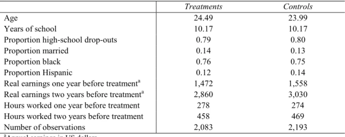
To assess the reliability of the experimental design, pre-treatment earnings and other demographic variables for male treatments and controls are presented in Table 1 (see also LaLonde (1986)). It can be seen that there are no significant differences to be found between these two groups: they were statistically equivalent in terms of observables, at least at the start of the programme. In the absence of non-random drop-out and with no alternative treatment offered and no changes in behaviour induced by the experiment, the controls constitute the perfect counterfactual to estimate the treatment impact.
Table 2 shows the earnings evolution for treatments and controls from a pre-programme year (1975), through the treatment period (1976–77), until the post-programme period (1978). It can be seen that the treatments’ and controls’ earnings were nearly the same before treatment, diverged substantially during the
TABLE 1
Comparison of Treatments and Controls: Characteristics for the NSWD Males
Treatments Controls
Age 24.49 23.99
Years of school 10.17 10.17
Proportion high-school drop-outs 0.79 0.80
Proportion married 0.14 0.13
Proportion black 0.76 0.75
Proportion Hispanic 0.12 0.14
Real earnings one year before treatmenta 1,472 1,558
Real earnings two years before treatmenta 2,860 3,030
Hours worked one year before treatment 278 274
Hours worked two years before treatment 458 469
TABLE 2
Annual Earnings of Male Treatments and Controls
Treatments Controls 1975 3,066 3,027 1976 4,035 2,121 1977 6,335 3,403 1978 5,976 5,090 Number of observations 297 425
programme and converged somewhat after it. The estimated impact one year after treatment is almost +$900.
Another interesting feature of the experimental data is the robustness to the choice of estimator. Table 3 (see Tables 5 and 6 of LaLonde (1986)) includes a set of estimates obtained using the control group and a number of other constructed comparison groups and based on different specifications that result in different estimation techniques. The choice of the ‘non-experimentally
TABLE 3
Estimated Treatment Effects for the NSWD Male Participants
using the Control Group and Comparison Groups from the PSID and the CPS-SSA
Comparison group Unadjusted difference of mean post-programme earnings Adjusted difference of mean post-programme earnings Unadjusted difference-in-differences Adjusted difference-in-differences Two-step estimator Controls 886 798 847 856 889 PSID 1 –15,578 –8,067 425 –749 –667 PSID 2 –4,020 –3,482 484 –650 — PSID 3 697 –509 242 –1,325 — CPS-SSA 1 –8,870 –4,416 1,714 195 213 CPS-SSA 2 –4,095 –1,675 226 –488 — CPS-SSA 3 –1,300 224 –1,637 –1,388 — Definitions:
PSID 1 — all male household heads continuously in the period studied (1975–78) who were less than 55 years old and did not classify themselves as retired in 1975.
PSID 2 — all men in PSID 1 not working when surveyed in the spring of 1976.
PSID 3 — all men in PSID 1 not working when surveyed in either the spring of 1975 or the spring of 1976. CPS-SSA 1 — all males based on Westat’s criterion except those over 55 years old.4
CPS-SSA 2 — all males in CPS-SSA 1 who were not working when surveyed in March 1976.
CPS-SSA 3 — all males in CPS-SSA 1 who were unemployed in 1976 and whose income in 1975 was below the poverty level.
4Westat’s criterion selects individuals who were in the labour force in March 1976 with nominal income less
determined’ comparison group is quite important, given the goal of reproducing the experimental setting as closely as possible. The aim is therefore to construct optimally a group of non-participants that closely reproduces what the participants would have been without the programme — which the group of controls is assumed to represent (experimental data). Given the observed characteristics, the comparison groups were drawn either from the Panel Study of Income Dynamics (those designated by PSID) or from the Current Population Survey, Social Security Administration (those designated by CPS-SSA).
Using comparisons from non-experimental control samples not only appears to change the results significantly but also raises the problem of dependence on the adopted specification for the earnings function and participation decision. We now turn to a general discussion of non-experimental methods in homogeneous and heterogeneous treatment effect models.
IV. METHODS FOR NON-EXPERIMENTAL DATA
The appropriate methodology for non-experimental data depends on three factors: the type of information available to the researcher, the underlying model and the parameter of interest. Datasets with longitudinal or repeated cross-section information support less restrictive estimators due to the relative richness of information. Not surprisingly, there is a clear trade-off between the available information and the restrictions needed to guarantee a reliable estimator.
Two estimators will be considered when only a single cross-section is available — namely, the instrumental variables (IV) and the two-step Heckman selection estimators. The IV method uses at least one variable that is related to the participation decision but otherwise unrelated to the outcome. It provides the required randomness in the assignment rule since the instrument is assumed to be in no way related to the outcome except through participation. Thus the relationship between the instrument and the outcome for different participation groups identifies the impact of treatment avoiding selection problems. The Heckman selection estimator is a two-step method that uses an explicit model of the selection process to control for the part of the participation decision that is correlated with the error term in the outcome equation.
If the available data are in a longitudinal or repeated cross-section format, difference-in-differences (diff-in-diffs) can provide a more robust estimate of the impact of the treatment. We will outline the conditions necessary for diff-in-diffs to estimate the impact parameter of interest reliably. In particular, we will also suggest an extension to overcome the common trends assumption. This assumption, which is crucial for the consistency of the estimator, states that the treatment and comparison groups are affected in the same way by macro shocks. This, of course, is often difficult to justify for comparison groups chosen from non-experimental data.
An alternative approach is the method of matching, which can be adopted with either cross-section or longitudinal data, although typically detailed individual information is required from before and after the programme for both the participant group and the non-participant comparison group. It will be shown that, with sufficiently detailed data, a simple ‘propensity score’ method of matching can often produce quite reasonable results. Matching deals with the selection process by constructing a comparison group of individuals with observable characteristics similar to those of the treated. One way of doing this is to model the probability of participation, estimate its value for each individual (called the propensity score) and match individuals with similar propensity scores. As will be explained below, a non-parametric propensity score approach to matching that combines this method with diff-in-diffs has the potential to improve the quality of non-experimental evaluation results significantly.
For each estimator, we will discuss its ability to identify the treatment impact in a homogeneous and a heterogeneous environment, as well as other specific advantages and disadvantages. The cross-section methodologies are introduced in the first two subsections: first the IV estimator is presented and then the Heckman selection estimator (Heckman, 1979). Subsection 3 discusses the diff-in-diffs approach and potential extensions when the common macro trends restriction does not hold. In subsection 4, we present the standard matching method and extensions to more refined techniques, such as the use of propensity scores to match and the use of diff-in-diffs along with matching.
1. The Instrumental Variables (IV) Estimator
Consider, first, the ‘homogeneous treatment effect’ case. The IV method requires the existence of at least one regressor exclusive to the decision rule, Z*,
satisfying the following three conditions: first, Z* determines programme
participation — that is, it has a non-zero coefficient in the decision rule; second, we can find a transformation, g, such that g(Z*) is uncorrelated with the error,
U, given the exogenous variables, X; finally, Z* is not completely (or almost)
determined by X. The variable(s) Z* is/are called the instrument(s), and it is a
source of exogenous variation used to approximate randomised trials: it provides variation that is correlated with the participation decision but does not affect the potential outcomes from treatment directly. Under the above conditions, the standard IV procedure may be applied, replacing the treatment indicator by g(Z*) and running a regression. An alternative is to use both Z* and X to predict
d, building a new variable, ˆd , which is used in the regression instead of d. This is a very simple estimator but it suffers from two main drawbacks. The first concerns the instrument choice. In the ‘treatment evaluation problem’, it is not easy to think of a variable that satisfies all the three assumptions required to
identify α. The difficulty lies, mainly, in the simultaneous requirements of ‘participation determination’ and ‘non-influence on the outcome of participation’. A commonly proposed solution, possible when longitudinal or past data are available, is to consider lagged values of some determinant variables. However, they are likely to be strongly correlated with future values, included in the outcome regression, and hence this is unlikely to solve the problem.
The second issue becomes clear when trying to evaluate the impact of training in a heterogeneous framework. To understand why, recall that, from (6), the error term is given by
(11) Uit +di iε =Uit +di(α αi− ). It is now evident that, even if *
i
Z is uncorrelated with Uit, the same is not true with respect to Uit +di(α αi− ) because *
i
Z determines di by assumption. The violation of this fundamental hypothesis invalidates the application of the IV methodology in a heterogeneous framework.
2. The Heckman Selection Estimator
This method is more robust than the IV estimator but also more demanding on assumptions about the structure of the model. As above, the simpler ‘homogeneous treatment effect’ case will be considered first. The main assumption required to guarantee reliable estimates of the treatment effect is the existence of at least one additional regressor in the decision rule. This regressor is required to have a non-zero coefficient in the decision rule equation and to be independent of the error term, V. Moreover, knowledge of or ability to estimate consistently the joint density of the distribution of the errors Uit and Vi —
( , )
i it i
h U V , say — is required. The rationale of this estimator is to control directly for the part of the error term in the outcome equation that is correlated with the participation dummy variable. The procedure uses two steps. In the first, the part of the error term Uit that is correlated with di is estimated. It is then included in the outcome equation and the effect of the programme is estimated in a second step. Of course, by construction, what remains of the error term in the outcome equation is not correlated with the participation decision.
Take, for example, the popular special case where Uit and Vi are assumed to follow a joint normal distribution. Adopting the standardisation σ =V 1, we may now write the conditional outcome expectation as
(12) ( ) ( | 1) ( ) ( ) ( | 0) , 1 ( ) i it i i i it i i Z E Y d Z Z E Y d Z φ γ β α ρ γ φ γ β ρ γ = = + + Φ = = − − Φ
where the last term on the right-hand side of each equation represents the expected value of the error term conditional on the participation variable, di. This is precisely what is missing from (1) when assignment to treatment is non-random, as described in subsection II(1). This new regressor deals with the part of the error term that is correlated with the decision process. By including it in the outcome equation, we are able to separate the true impact of treatment from the selection process, which accounts for the differences between participants and non-participants. Thus it is possible to estimate α, the Heckman selection estimator for the selection model, by replacing γ with ˆγ (obtained from regressing IN on Z) and running a least squares regression on (12).5
(a) The Heckman Selection Estimator: Choice-Based Samples
One advantage of the two-step procedure in the ‘homogeneous treatment effect’ case relates to its robustness to choice-based sampling. This is the kind of non-randomness obtained when drawing the comparison group (non-treated) from the population. Usually, the sample proportion of treated ( *
t
p ) differs from the population one (pt). The treated are likely to be over-represented in the sample, resulting in a non-zero expectation of the outcome error term:
(13) * ( | 1) (1 *) ( | 0) 0.
t it i t it i
p E U d = + −p E U d = ≠
Robustness is achieved by controlling for the part of Uit that is correlated with
i
d . In fact, since the remaining error is orthogonal to di, it is unaffected by this type of stratification.
(b) The Heckman Selection Estimator: Heterogeneous Treatment Effects
Now suppose that the treatment impact differs across agents. The outcome equation becomes
(14) Yit = +β αTdi+{Uit +di[εi−E( |εi di=1)]}= +β αTdi+ξit.
5For a more detailed description of this estimator, see the Appendix.
The two-step procedure requires knowledge of the joint density of Uit, Vi and
i
ε . Continuing to assume a joint normal distribution (σ =V 1), (15) 1/ 2 ( , , ) 1/ 2 ( , ) ( ) ( ) ( | 1) Corr( , )Var( ) ( ) ( ) ( ) ( ) ( | 0) Corr( , )Var( ) . 1 ( ) 1 ( ) i i it i it i i it i U V i i i i it i it i it U V i i Z Z E d U V U Z Z Z Z E d U V U Z Z ε φ γ φ γ ξ ε ε ρ γ γ φ γ φ γ ξ ρ γ γ = = + + = Φ Φ − − = = = − Φ − Φ
Hence the outcome regression equation is
(16) ( , , ) ( ˆ) (1 ) ( , ) ( ˆ) , ˆ ˆ ( ) 1 ( ) i i it i T U V i U V it i i Z Z Y d d Z Z ε φ γ φ γ β α ρ ρ δ γ γ − = + + + − + Φ − Φ
which consequently identifies αT.
However, this method is unable to identify α, the effect of training if individuals were randomly assigned to treatment. In fact, if α is the parameter of interest, the appropriate equation is
(17) Yit = +β αdi+(Uit +di iε )= +β αdi+ηit.
Notice that the error term for the treated no longer has a zero expectation. Formally, (18) ( , , ) ( , ) ( ) ( | 1) ( | 1) ( | 1) ( ) ( ) ( | 0) ( | 0) . 1 ( ) i it i it i i i i i U V i i it i it i U V i Z E d E U d d E d Z Z E d E U d Z ε φ γ η ε ε ρ γ φ γ η ρ γ = = + = = = + Φ − = = = = − Φ
Therefore the outcome equation is given by
(19) ( , , ) ( , ) ˆ ( ) ( | 1) ˆ ( ) ˆ ( ) (1 ) , ˆ 1 ( ) i it i i i U V i i i U V it i Z Y d E d Z Z d Z ε φ γ β α ε ρ γ φ γ ρ δ γ = + + = + Φ − + − + − Φ
which is exactly the same equation as the one obtained when trying to estimate
T
3. The Difference-in-Differences (Diff-in-Diffs) Estimator
If longitudinal or repeated cross-section information is available, it is possible to estimate the treatment effect consistently without having to impose such restrictive conditions. To apply the diff-in-diffs estimator, at least one pre-programme set and one post-pre-programme set of observations are required. Let t0 and t1 denote the pre- and post-programme periods for which data are available.
The diff-in-diffs estimator measures the excess outcome growth for the treated compared with the non-treated. Formally, abstracting from other regressors besides the treatment indicator,
(20)
1 0 1 0
ˆ ( T T) ( C C),
DID Yt Yt Yt Yt
α = − − −
where YT and YC are the mean outcomes for the treatment and comparison
(non-treatment) groups, respectively.
(a) The Diff-in-Diffs Estimator: Heterogeneous Treatment Effects
Where the impact of treatment is heterogeneous, provided the above conditions are verified, the diff-in-diffs estimator recovers the impact of the treatment on the treated: (21) 1 0 1 0 ˆ ( ) [ ( | 1) ( | 1)] [ ( | 0) ( | 0)] . DID T t t t t T E E U d E U d E U d E U d α β α β β β α = + + = − − = − + = − − = =
That is, the effect of treatment on the treated is identifiable, but not the population impact. Intuitively, this happens because the unobserved component of the treatment impact enters in the model as a temporary individual-specific effect that determines participation.
(b) The Diff-in-Diffs Estimator: The Common Trends and Time-Invariant Composition Assumptions
In contrast to the IV and Heckman selection estimators, no exclusion restrictions appear to be required for the diff-in-diffs estimator. In fact, there is no need for any regressor in the decision rule. Even the outcome equation does not have to be specified as long as the treatment impact enters additively. However, strong restrictions on common trends and error composition are implicit, which we now describe.
Consider the following decomposition of the unobservables, Uit: (22) Uit = + +φ θ µi t it,
where φi is an individual-specific effect, constant over time, θt is a common macroeconomic effect, the same for all agents, and µit is a temporary individual-specific effect. Notice that, if the expectation of Uit conditional on the treatment status depends on the temporary individual-specific effect, µit, diff-in-diffs is inconsistent. This estimator is, however, able to control for the other two error-term components as they cancel out on subtraction. As is straightforward to verify, a separability condition between individual and temporal effects has to be assumed:
(23) E U d( it| )i =E( | )φi di +θt.
Even simpler than this estimator, a simple difference method could be applied if the only unobservable term is φi, the constant individual-specific effect. The estimator (24) 1 0 ˆ ( T T) D Yt Yt α = −
would suffice to identify α consistently.
There are two main weaknesses of the diff-in-diffs approach. The first relates to the lack of control for unobserved temporary individual-specific components that influence the participation decision. In fact, the following can be written: (25)
1 0 1 0
ˆ
( ) ( t t | 1) ( t t | 0).
E α = +α E µ −µ d= −E µ −µ d =
To illustrate the conditions under which such inconsistency might arise, suppose we are interested in evaluating a training programme in which enrolment is more prone to happen if a temporary dip in earnings occurs just before the programme takes place (so-called Ashenfelter’s dip; see Heckman and Smith (1994)). A faster earnings growth is expected to occur among the treated, even without programme participation. Thus the diff-in-diffs estimator is likely to overestimate the impact of treatment. Also, if only repeated cross-section data are available, it may be difficult to control for the before–after comparability of the groups under this type of selection into the programme. That is, if individuals select into the programme according to some unknown rule, and repeated cross-section data are being used, the assumption that ( | )Eφi di is constant over time for each group may be too strong because the composition of the groups may change over time and be affected by the intervention.
The second weakness occurs if the macro effect has a differential impact across the two groups. This happens when the treatment and comparison groups
them react differently to common macro shocks. This motivates the differential-trend-adjusted diff-in-diffs estimator that is presented below.
(c) The Diff-in-Diffs Estimator: Adjusting for Differential Trends Suppose that the comparison group and target group actually satisfy (26) (E U dit| )i =E( | )φi di +kg tθ ,
where the kg acknowledges the differential macro effect across the two groups. Now it can be seen that the diff-in-diffs estimator identifies
(27)
1 0
ˆ
( DID) ( T C)( t t ), E α = +α k −k θ −θ
where T and C refer to the treatment and control groups, respectively. This clearly only recovers the true effect of the programme when kT =kC.
Now suppose we take another time interval t* to t**, over which a similar macro trend has occurred. Precisely, we require a period for which the macro trend matches the term
1 0
(kT −kC)(θt −θt ) in (27). It is likely that the most recent cycle is the most appropriate, earlier cycles possibly having systematically different effects across the target and comparison groups.
The differentially adjusted estimator proposed by Bell, Blundell and Van Reenen (1999), which takes the form
(28)
1 0 1 0 ** * ** *
ˆ [( T T) ( C C)] [( T T) ( C C)],
TADID Yt Yt Yt Yt Yt Yt Yt Yt
α = − − − − − − −
will now consistently estimate α. 4. The Matching Estimator
The matching method is a non-parametric approach to the problem of identifying the treatment impact on outcomes. It is more general in the sense that no particular specification has to be assumed. Moreover, it can be combined with other methods, producing more accurate estimates and allowing for less restrictive assumptions. However, it too rests on strong assumptions and particularly heavy data requirements.
The main purpose of matching is to re-establish the conditions of an experiment when no such data are available. As discussed earlier, with total random assignment within one group, one could compare the treated and the non-treated directly, without having to impose any structure on the problem. With the matching method, the construction of a correct sample counterpart for the missing information on the treated outcomes had they not been treated
consists in pairing each programme participant with members of a comparison group (non-treated). Under the matching assumption, the only remaining difference between the two groups is programme participation.
(a) The Matching Estimator: General Method
To illustrate the matching solution in a more formal way, consider a general specification of the outcome function,
(29) ( ) ( ) , T T T C C C Y g X U Y g X U = + = +
where YT and YC are the outcomes of the treated and the non-treated
(comparison group), which can be written as a function of the set of observables, X, plus the unobservable term, UT or UC. Note that we allow for different
outcome functions according to the participation decision.
As above, the most common goal of evaluation is to identify the impact of the treatment on the treated:
(30) ( T C | , 1).
T E Y Y X d
α = − =
The solution advanced by matching is based on a fundamental assumption of conditional independence between non-treated outcomes and programme participation:
(31) | .YC ⊥d X
This assumption states that the outcomes of the non-treated are independent of the participation status, d, once one controls for the observable variables, X. That is, given X, the non-treated outcomes are what the treated outcomes would have been had they not been treated or, in other words, selection occurs only on observables.6 For each treated observation, YT, we can look for a non-treated
(set of) observation(s), YC, with the same X-realisation. With the matching
assumption, this YC constitutes the required counterfactual. Actually, this is a
process of rebuilding an experimental dataset which, in general, places strong requirements on data collection.
Additionally, matching also assumes that 0 Prob(< d=1| ) 1X < in order to guarantee that all treated agents have a counterpart in the non-treated population, and that anyone constitutes a possible participant. However, this does not ensure
that the same happens within any sample, and it is, in fact, a strong assumption when programmes are directed to tightly specified groups.
Let S be the set of all possible values the vector of explanatory variables, X, may assume. It is called the ‘support of X’. Let S* be the common support of X,
or the space of X that is simultaneously observed among participants and non-participants for the specific dataset being used. Assuming the above described conditions, a subset of comparable observations is formed from the original sample, and with those a consistent estimator for the treatment impact on the treated, αT, is the empirical counterpart of
(32) * * ( | , 1)d ( | 1) . d ( | 1) T C S S E Y Y X d F X d F X d − = = =
∫
∫
The numerator of the above expression represents the expected gain from the programme among the subset of participants who are sampled and for whom one can find a comparable non-participant (that is, over S*). To obtain a measure of
the impact of the treatment on the treated, individual gains must be integrated over the distribution of observables among participants and re-scaled by the measure of the common support, S*. The fraction therefore represents the
expected value of the programme effect in the common support of X, S*. It is
simply the mean difference in outcomes over the common support, appropriately weighted by the distribution of participants. If the second assumption is fulfilled and the two populations are large enough, the common support is the entire support of both.
As should now be clear, the matching method avoids specifying a particular form for the outcome equation, decision process or either unobservable term. We simply need to ensure that, given the right observables, X, the observations of non-participants are statistically what the observations of the treated would be had they not participated. Under a slightly different perspective, it might be said that we are decomposing the treatment effect in the following way:
(33) ( | , 1) [ ( | , 1) ( | , 0)] [ ( | , 1) ( | , 0)], T C T C C C E Y Y X d E Y X d E Y X d E Y X d E Y X d − = = = − = − = − =
the latter right-hand-side term being the bias conditional on X, which is assumed to be zero. The technique is to replace the unobserved outcomes of the participants had they not been treated with the outcomes of non-participants with the same X-characteristics.
(b) The Matching Estimator: The Role of the Participation Decision
Up to now, we have been differentiating individuals based on participation. However, the structural difference should rely on the participation decision. The participation decision, though, is not observable among non-participants. These form a mixture of those who, if offered the programme, would have decided to participate and those who would have decided not to. All the participants, however, were willing to be treated when the programme was offered to them. In such case, the outcome equations would be
(34) 1 0 ( ) ( ) [ (1 ) ], T T T C C D C D C Y g X U Y g X d U d U = + = + + −
where dD is a dummy variable standing for participation decision and 1C
U and
0 C
U are the outcome error terms for non-participants who would and would not be willing to participate, respectively.
The parameter of interest — the mean impact of treatment — is (35) E Y( T −YC | ,X d = =1) g XT( )−g XC( )+E U( T −U1C | ,X dD =1).
Therefore there are two possibilities underlying matching assumptions:
*
Prob(dD =1| ) 1X = ∀ ∈X S or *
0 1
( C| ) ( C| )
E U X =E U X ∀ ∈X S . The first hypothesis states that X completely determines the participation decision: anyone characterised by a value of X on the common support, S*, would be willing to
participate if offered the programme. This is the desired outcome if one is willing to reconstruct an experimental setting, since it states that X is enough to build up a comparison group with the desired similarities to the treatment group. The second assumption states that, at least as far as the unobservables are concerned, the two comparison groups defined by the participation decision are equal. This means that participation decisions are being based on observables alone and the matching assumption (31) follows.
Under this formulation, matching is always preferable to random sampling if it increases Prob(dD=1) among comparisons and/or if it brings
1
( C) E U and
0
( C)
E U closer in the support, S*. Any of these conditions causes the comparison
group to become more similar to the treatment group in the sense that at least a part of the difference is being controlled for by the observables. This is the advantage of applying matching under such circumstances.
(c) The Matching Estimator: The Use of the Propensity Score
It is clear that when a wide range of variables X is in use, matching can be very difficult due to the high dimensionality of the problem. A more feasible alternative is to match on a function of X. Usually, this is carried out on the propensity to participate, given the set of characteristics, X: P X( i)=
Prob(di=1|Xi), which is the propensity score. Its use is usually motivated by Rosenbaum and Rubin’s (1983 and 1984) result. It is shown that, under the (matching) assumptions
(36) (Y YT, C)⊥d X| and 0 Prob(< d=1| ) 1,X <
the conditional independence remains valid if controlling for P(X) instead of X: (37) (Y YT, C)⊥d P X| ( ).
More recently, a study by Hahn (1998) shows that the propensity score is ancillary for the estimation of the average effect of treatment on the population. However, it is also shown that knowledge of the propensity score may improve the efficiency of the estimates of the average effect of treatment on the treated. Its value for the estimation of this latter parameter lies in the ‘dimension reduction’ feature.
When using the propensity score, the comparison group for each treated individual is chosen with a pre-defined criterion (established by a pre-defined measure) of proximity. Having defined the neighbourhood for each treated observation, the next issue is that of choosing the appropriate weights to associate the selected set of non-treated observations with each participant one. Several possibilities are commonly used, from a unity weight to the nearest observation and zero to the others, to equal weights to all, or kernel weights, which account for the relative proximity of the non-participants’ observations to the treated ones in terms of P(X).
In general, the form of the matching estimator is given by
(38) ˆMM i ij j i, i T j C Y W Y w α ∈ ∈ = −
∑
∑
where Wij is the weight placed on comparison observation j for individual i and
i
w accounts for the reweighting that reconstructs the outcome distribution for the treated sample. For example, in the nearest neighbour matching case, the estimator becomes
(39) ˆMM ( i j) 1 , i T T Y Y N α ∈ =
∑
−where j is the nearest neighbour in terms of P(X) in the comparison group to i in the treatment group. In general, kernel weights are used for Wij to account for the closeness of Yj to Yi.
(d) The Matching Estimator: Parametric Approach
Specific functional forms assumed for the g-functions in (29) can be used to estimate the impact of treatment on the treated over the whole support of X, reflecting the trade-off between the structure one is willing to impose in the model and the amount of information that can be extracted from the data. To estimate the impact of treatment under a parametric set-up, one needs to estimate the relationship between the observables and the outcome for the treatment and comparison groups and predict the respective outcomes for the population of interest. A comparison between the two sets of predictions supplies an estimate of the impact of the programme. In this case, one can easily guarantee that outcomes being compared come from populations sharing exactly the same characteristics.
When a linear specification is assumed with common coefficients for treatments and controls, so that
(40) , T T C Y X d U Y X U β α β = + + = +
not even the common support requirement is needed to estimate the impact of treatment on the treated — a simple OLS regression using all information on the treated and non-treated will consistently identify αT.
(e) The Matching Estimator: Drawbacks
It is likely that matching does not succeed in finding a non-treated observation with similar propensity score for all the participants. That is, for some observations, we might be unable to find the right counterfactual, which means that the common support is just a subset of the complete treated support. If the impact of treatment is homogeneous, at least within the treatment group, no additional problems appear besides the loss of information. Note, however, that the setting is general enough to include the heterogeneous case. If the impact of training is heterogeneous within the treatment group itself and the counterfactual is more difficult to obtain for some subgroup(s) of the participants, it may be
impossible to identify αT . In other words, if the matching process leads to a considerable loss of observations, the estimator is limited by the loss of information and is only consistent for the common support. In the ‘heterogeneous response’ case, if the expected impact of participation differs across the treated, it is possible that the estimated impact does not represent the mean outcome of the programme.
Another potential problem with matching is the (heavy) requirements on data. To guarantee that assumption (31) is verified, it is important to obtain the relevant information to distinguish potential participants from others, which is not always easy. On the other hand, the more detailed the information is, the harder it is to find a similar control and the more restricted the common support becomes. That is, the correct balance between the quantity of information to use and the share of the support covered may be difficult to achieve.
(f) A Bias Decomposition
The bias term can be decomposed into three distinct parts: (41) Bias E Y= ( C | ,X d= −1) E Y( C | ,X d= = +0) B1 B2+B3,
where B1 represents the bias component due to non-overlapping support of X,
2
B is the error part due to misweighting on the common support of X as the resulting empirical distributions of treated and non-treated are not the same even when restricted to the same support, and B3 is the true econometric selection bias resulting from ‘selection on unobservables’. Through the process of choosing and reweighting observations, matching corrects for the first two sources of bias, and the third term is assumed to be zero.
(g) Matching and Diff-in-Diffs
The assumption of conditional independence between the error term in the outcome equation and the training status (depicted by (31)) is quite strong if it is possible that individuals decide according to their forecast outcome. However, if matching is combined with diff-in-diffs, there is scope for an unobserved determinant of participation as long as it can be represented by separable individual- and/or time-specific components of the error term. To clarify the exposition, let us now assume the following model specification:
(42) , T T T T it t i t it C C C C it t i t it Y g Y g φ θ µ φ θ µ = + + + = + + +
which differs from (29) by the composition assumed for the error term and by explicitly acknowledging that the function g may change over time.7
If performing matching on the set of observables X within this setting, the conditional independence assumption (31) can now be replaced by
(43)
1 0 | ,
C C
t t
Y −Y ⊥d X
where t0 and t1 stand for the before- and after-programme time periods. Given (42), assumption (43) is equivalent to (44) 1 0 1 0 ( C C) ( C C) | . t t t t g −g + θ −θ ⊥d X
The main matching hypothesis is now stated in terms of the before–after evolution instead of levels. If both terms of the sum in (44) are conditionally independent of the participation decision, then (44) is verified. It means that controls have evolved from a pre- to a post-programme period in the same way treatments would have done had they not been treated. This happens both on the observable component of the model and on the unobservable time trend.
The effect of the treatment on the treated can now be estimated over the common support of X, S*, using an extension to (38):
(45) 1 0 1 0 ˆLD ( ) ( ) , MMDID it it ij jt jt i i T j C Y Y W Y Y w α ∈ ∈ = − − −
∑
∑
where LD denotes ‘longitudinal data’ and MMDID denotes ‘method of matching with difference-in-differences’.
Quite obviously, this estimator requires longitudinal data to be applied. It is, however, possible to extend it for the repeated cross-sections data case. If only repeated cross-sections are available, one must perform matching three times for each treated individual after being treated: to find the comparable treated before the programme and the controls before and after the programme. If the same assumptions apply, one can estimate the effect of treatment on the treated using the following estimator:
(46)
1 0 0 1 1 0 0
1 0 1 1
ˆRCS T C C ,
MMDID it ijt it ijt jt ijt jt i
i T j T j C j C Y W Y W Y W Y w α ∈ ∈ ∈ ∈ = − − −
∑
∑
∑
∑
7Of course, this latter point is only important when comparing different periods, as done within the diff-in-diffswhere RCS denotes ‘repeated cross-section’, T0, T1, C0 and C1 stand for the treatment and control groups, before and after the programme, respectively, and
G ijt
W represent the weights attributed to individual j in group G (where G = C or T) and at time t when comparing with treated individual i.8
V. SOME EMPIRICAL STUDIES
In this section, we draw on two studies, one from the UK and one from the US, to illustrate some of the non-experimental techniques presented in this review. In the influential study by LaLonde (1986), it was concluded that none of the used econometric methodologies estimate accurately the treatment impact when only non-experimental data are available.9 However, there are two potential issues with the LaLonde study (see Heckman, Ichimura and Todd (1997)). The first concerns the questionnaires: controls and comparisons answered different questions, based on different definitions. Second, the comparison group was not guaranteed to operate in the same labour market as the treatments, and hence different macro effects may influence each group’s behaviour.
The studies presented below illustrate that the methods we have described for non-experimental data can provide good evaluation information if carefully handled. Both illustrations concern labour market programmes, the first taking place in the UK and the second in the US.
1. Diff-in-Diffs and Differential Trends: The New Deal Evaluation in the UK The New Deal for Young People is a recent initiative of the UK government to help young unemployed people make their way into or back to work. The programme is targeted at the 19- to 24-year-old long-term unemployed. Participation is compulsory, so that every eligible individual is due to participate under the threat of losing entitlement to benefits. The criteria for eligibility are simple: every individual aged 19–24 by the time of completion of the sixth month on jobseeker’s allowance (JSA) is immediately assigned to the programme and starts receiving treatment. Given the stated rules, the programme can be classified as one of global implementation, being administered to literally everyone in the UK meeting the eligibility criteria. Indirect effects are therefore expected. The nature of these effects will be discussed below.
Treatment is composed of three steps. On assignment to the programme, the individual starts an intensive job-search assistance period, called the Gateway, which lasts for up to four months. The second stage is composed of a six-month spell in subsidised employment or up to 12 months in full-time education or 8For a more detailed discussion with an application of the combined matching and diff-in-diffs estimator, see
Blundell, Costa Dias, Meghir and Van Reenen (2000).
training. The former involves a payment of a subsidy to the employer while the employee receives the offered wage. For the latter, the individual receives an amount equivalent to the JSA payment and may be eligible for special grants in order to cover exceptional expenses. Once the option period is over, individuals who remain unemployed enrol in a new period of intense job search, the Follow-Through, which takes up to 13 weeks.
The programme was launched in the whole UK by April 1998. There was, however, a previous three-month experimental period (January 1998 to March 1998) when the programme was tried in 12 regions, called Pathfinders. The goal was to perform a three-month experiment with the Pathfinders, having as counterfactual the rest of the UK or some regions that would match the Pathfinders more closely. Clearly, identification of the treatment effect under these conditions requires stronger assumptions than when the experiment is run within regions using random assignment. As will be discussed, the problem relates to the fact that the counterfactual must be drawn either from a different labour market or from a group with different characteristics operating in the same labour market. Different types of hypotheses will be studied below.
The analysis that follows is based on the study by Blundell, Costa Dias, Meghir and Van Reenen (2000). It uses the publicly available 5 per cent sample of the whole population claiming JSA in the UK since 1982 (JUVOS). This database includes a small set of demographic variables and the start and exit dates from the claimant count, making it possible to reconstruct the unemployment history of the individuals. The outflow from the claimant count is the outcome of interest, the choice having been determined by the availability and quality of the data used (outflows by destination are also covered in Blundell, Costa Dias, Meghir and Van Reenen (2000), but since the necessary information is only available since late 1996, we have chosen to focus here on the outflows to all destinations taken together). Also, since the programme is very recent, it is still not possible to make a long-run analysis of the effect of participation. Given this, we will use two measures in trying to evaluate the effect of the programme: outflows from the claimant count within, respectively, two and four months of completion of the sixth month on unemployment subsidy.
The rest of this section goes as follows. We start by briefly discussing the nature of the experiment. The second subsection addresses the problem of choosing and assessing a control group. We then present the estimates of the effect of the programme, and finally we discuss these results and their potential problems, mainly related to the nature of the programme.
(a) The Experimental Period
We will present a detailed analysis of the experimental period of the New Deal for Young People. The experiment was undertaken during the first three months