Systematic Extreme Downside Risk
Richard D. F. Harris, University of Exeter Linh H. Nguyen, De Montfort University
Evarist Stoja, University of Bristol
September 2018
Abstract
We propose new systematic tail risk measures constructed using two different approaches. The first is a non-parametric measure that captures the tendency of a stock to crash at the same time as the market, while the second is based on the sensitivity of stock returns to innovations in market crash risk. Both tail risk measures are associated with a significantly positive risk premium after controlling for other measures of downside risk, including downside beta, coskewness and cokurtosis. Using the new measures, we examine the relevance for investors of the tail risk premium over different horizons.
Keywords: Asset pricing, Tail risk, Comoments, Value at Risk, Systematic risk. JEL codes: C13, C31, C58, G01, G10, G12.
Address for correspondence: Professor Richard D. F. Harris, Rennes Drive, Exeter EX4 4ST, UK, email: [email protected]. Linh H. Nguyen, Leicester Business School, The Newarke, Leicester, LE1 9BH, UK, email: [email protected]. Evarist Stoja, School of Economics, Finance and Management, University of Bristol, 8 Woodland Road, Bristol, BS8 1TN, UK. Email: [email protected]. We would like to thank the Editor and an anonymous referee for their insightful comments that have greatly helped to improve the paper. Parts of this paper were written while Evarist Stoja was a Houblon-Norman Fellow at the Bank of England whose hospitality is gratefully acknowledged. The views expressed here are solely our own and do not necessarily reflect those of the Bank of England.
2 1. Introduction
The turbulence of financial markets over the last few decades has highlighted the importance of tail risk for asset pricing. Many studies have documented the significant impact of this type of risk on expected returns. Rietz (1988) shows that the inclusion of a crash state in a three-state model plays an important role in generating the observed risk premium for the US equity market for reasonable levels of risk aversion and consumption growth volatility. His findings are confirmed by Barro (2006) in a framework of consumption growth with a crash term and a specific measure of disaster risk. Their framework is extended by Gillman et al. (2015), who model rare disasters by the shifts in both the growth rate and the growth persistence of consumption and dividends. Further, Gabaix (2012) and Wachter (2013) account for time-varying disaster risk as well as the relative performance of different assets in times of distress. However, the small number of actual economic disasters is a practical challenge for further development of measures of crash risk.
An alternative approach to examining the role of tail risk is to directly investigate the impact of the tail of the return distribution on expected returns. Owing to the fact that asset returns are generally observable at high frequencies, measures corresponding to any aspect of the return distribution can be readily constructed, and moment-based risk measures such as variance, skewness and kurtosis have all been shown to significantly influence stock returns (see, for example, Arditti, 1971; Arditti and Levy, 1975; Ang et al., 2006b; Boyer et al., 2010; Chang et al., 2013; Conrad et al., 2013). In a portfolio context, many studies have modelled the impact of systematic moment risks, such as CAPM beta, coskewness and cokurtosis, on returns. For example, Kraus and Litzenberger (1976) and Harvey and Siddique (2000) develop a three-moment CAPM and find that the coskewness is significantly related to asset returns. Dittmar (2002) incorporates investor preferences over the first four moments of returns to derive a cubic form of the pricing kernel and finds that cokurtosis also affects returns. Chiao et al. (2003) develop a conditional four-moment CAPM to investigate the relevance of coskewness and cokurtosis in up and down market states. They present evidence of significant risk premia associated with these states, especially with the up market state. Comparing the Australian market with the US market, Doan et al. (2010) show that the relative significance of coskewness and cokurtosis is influenced by the skewness and kurtosis features of stock returns. Iqbal et al. (2010) augment the Fama and French (1993) model with a cubic market factor that accounts for cokurtosis and find that the model outperforms a
3
number of competing models. Moreover, Chung et al. (2006) demonstrate that higher comoments of up to order ten collectively capture the Fama and French (1993) factors.
In contrast with the findings for moment-based risk measures, which offer indirect evidence on the importance of tail risk in asset pricing, direct evidence on the role of tail risk is sparse. This is especially true for the systematic component, namely the tail risk of individual stocks that is determined by market-wide factors, and hence cannot be eliminated through portfolio diversification. Bali and Cakici (2004) examine the influence of tail risk on cross-sectional returns using Value at Risk (VaR) but do not separately consider its systematic and idiosyncratic components. Huang et al. (2012) show that idiosyncratic tail risk is significant in determining stock returns, using a measure of idiosyncratic tail risk on the residuals of the Carhart (1997) four-factor model. However, they do not shed light on the importance of systematic tail risk for individual stock returns. Chabi-Yo et al. (2018) propose a systematic tail risk measure, Lower Tail Dependence (LTD), based on the estimated crash sensitivity of an individual stock to a market crash. The risk premium corresponding to this measure is positive since stocks with high LTD tend to offer low returns when investors’ wealth is low. However, the LTD is based on a combination of a number of parametric copulas and thus its estimation is computationally intensive, which may limit its usefulness in practice. In a related study, Meine et al. (2016) present evidence that tail dependence is significantly priced in CDS markets, especially during financial crises. Oordt and Zhou (2016) propose a new systematic tail risk measure that captures the sensitivity of asset returns to market returns conditional on market tail events and show that this measure is associated with future stock returns. However, their measure is not associated with a significantly positive tail risk premium.
A number of studies examine the relationship between tail risk and returns at the market level, thus bypassing the need to decompose risk into its systematic and idiosyncratic components. Bali et al. (2009) find a positive relationship between the expected monthly market VaR and the corresponding monthly market returns. Bollerslev and Todorov (2011) estimate an ‘Investor Fear Index’ for the market and show that it is associated with a significant premium. Kelly and Jiang (2014) develop a market tail risk measure based on the common component of the tail risk of individual stocks and show that it has significant predictive power for market returns. Bali et al. (2014) introduce a hybrid tail risk measure that incorporates both market-wide and firm-specific components and show that this yields a robust and significantly positive tail risk premium.
4
Given the conflicting evidence regarding the tail risk premium, in this paper, we contribute to this literature by proposing two new measures of systematic tail risk and show that each is associated with a significant risk premium. The first measure is based on the tendency of stock returns to crash at the same time as the market, while the second is based on the sensitivity of stock returns to market tail risk. We first investigate the relationship between expected returns and systematic tail risk by sorting all stocks in the NYSE, AMEX and NASDAQ into quintiles based on each of these new measures. We observe an almost monotonic increase in average returns from the lowest to the highest risk quintile, and the alphas of long-short strategies for these portfolios are significantly positive, confirming the economic significance of the systematic tail risk premium. We conduct a Fama and MacBeth (1973) cross-sectional analysis for the systematic tail risk measures, controlling for a large set of other risk measures including downside beta, upside beta, size, book-to-market, volatility, liquidity, past returns and systematic higher moments. The cross-sectional analysis confirms the significant and positive tail risk premium of the proposed tail risk measures as well as their ability to predict future returns. Thus, our study provides evidence on the incremental information content of tail risk that is not fully captured by other risk factors in the literature. Our results are robust to different measures of tail risk, different estimation methods and different cut-off thresholds for the tail of the return distribution. Additionally, our tail risk sensitivity measure relies on daily observations of market tail risk and can therefore be estimated for very short horizons. It thus overcomes one of the most challenging problems in the tail risk literature – the trade-off between the low frequency of tail risk measures when using a non-overlapping estimation window and the low variability of the measure when using an overlapping window. This feature enables us to investigate the impact of systematic tail risk on returns over horizons of different lengths, revealing interesting patterns in the dynamics of tail risk.
The remainder of this paper is organized as follows. Section 2 introduces the new systematic tail risk measures. Sections 3 and 4 utilize these proposed measures to investigate the relationship between tail risk and expected returns. Section 5 presents the results of the robustness tests. Section 6 summarizes the main findings and offers some concluding remarks.
5 2. Systematic Tail Risk Measures
In this section, we propose two new measures to estimate the systematic tail risk of an asset. The first measure captures the tendency of an asset to crash given that the market has crashed, while the second is based on investors’ demand to hedge against tail events and the idea that a systematic tail risk measure should capture the sensitivity of stock returns to market tail risk.
2.1.Extreme Downside Correlation
A systematic tail risk measure should capture the performance of asset returns conditional on a market tail event. An asset that performs well when the market crashes is more attractive to investors as it offers high returns when their wealth is low and the marginal utility of consumption is high. On the other hand, assets that tend to crash at the same time as the market are risky, and thus investors require a higher risk premium to hold them. This is the basis for the LTD measure of Chabi-Yo et al. (2018). Their measure captures the propensity of an asset to experience a tail event given the occurrence of a market tail event. Specifically, for an asset 𝑖 with excess return 𝑅𝑖, and the stock market excess return 𝑅𝑚, the LTD is defined as:
𝐿𝑇𝐷 = 𝑙𝑖𝑚
𝑞→0+𝑃𝑙(𝑞) (1)
where
𝑃𝑙(𝑞) = 𝑃𝑟[𝑅𝑖 < 𝐹𝑅−1𝑖 (𝑞)|𝑅𝑚 < 𝐹𝑅−1𝑚(𝑞)] (2)
In Equation (2), 𝐹−1(𝑞) denotes the quantile function of a CDF 𝐹 corresponding to the quantile level 𝑞. The LTD measure is therefore estimated from the joint distribution of the asset return and the market return. Given the non-normality and crash-clustering features of the joint distribution of returns, Chabi-Yo et al. (2018) estimate the LTD using copulas and find that the resulting measure is associated with a significantly positive risk premium. Their method is also used to capture the significant tail risk premium in international stock markets worldwide in Weigert (2016). However, as noted above, this measure is computationally intensive as it is based on a combination of a number of parametric copulas, which may limit its usefulness in practice.
6
We propose a simple non-parametric measure of systematic tail risk that captures the propensity for an asset to crash at the same time as the market. The measure is based on the comoment between the asset return and the market return, adapted to focus on the tail of joint return distribution. The kth comoment is given by (see, for example, Ang et al., 2006a; Guidolin and Timmermann, 2008):
𝑘𝑡ℎ 𝑐𝑜𝑚𝑜𝑚𝑒𝑛𝑡 𝑜𝑓 𝑎𝑠𝑠𝑒𝑡 𝑖 = 𝐸[(𝑅𝑖−𝜇𝑖)(𝑅𝑚−𝜇𝑚)𝑘−1]
𝑣𝑎𝑟(𝑅𝑖)1 2⁄ 𝑣𝑎𝑟(𝑅𝑚)(𝑘−1) 2⁄ (3) where 𝑘 = 3 corresponds to coskewness:
𝑐𝑜𝑠𝑘𝑒𝑤𝑛𝑒𝑠𝑠 𝑜𝑓 𝑎𝑠𝑠𝑒𝑡 𝑖 = 𝐸[(𝑅𝑖−𝜇𝑖)(𝑅𝑚−𝜇𝑚)2]
𝑣𝑎𝑟(𝑅𝑖)1 2⁄ 𝑣𝑎𝑟(𝑅𝑚) (4) and 𝑘 = 4 corresponds to cokurtosis:
𝑐𝑜𝑘𝑢𝑟𝑡𝑜𝑠𝑖𝑠 𝑜𝑓 𝑎𝑠𝑠𝑒𝑡 𝑖 = 𝐸[(𝑅𝑖−𝜇𝑖)(𝑅𝑚−𝜇𝑚)3]
𝑣𝑎𝑟(𝑅𝑖)1 2⁄ 𝑣𝑎𝑟(𝑅𝑚)3 2⁄ (5)
We shift the domain of the comoment from the whole distribution of returns to the 𝛼-quantile of the distribution. We set 𝑘 = 2 to yield the Extreme Downside Correlation (hereafter EDC), defined as:
𝐸𝐷𝐶 = 𝐸[(𝑅𝑖−𝜇𝑖)𝛼(𝑅𝑚−𝜇𝑚)𝛼]
𝐸((𝑅𝑖−𝜇𝑖)𝛼2)1 2⁄ 𝐸((𝑅𝑚−𝜇𝑚)𝛼2)1 2⁄
(6)
where 𝑅𝑖 and 𝑅𝑚 are the excess returns of asset 𝑖 and the market, 𝜇𝑖 and 𝜇𝑚 are the mean of
𝑅𝑖 and 𝑅𝑚, (𝑅𝑖 − 𝜇𝑖)𝛼 is equal to (𝑅𝑖 − 𝜇𝑖) if 𝑅𝑖 is smaller than its 𝛼-quantile and 0 otherwise, (𝑅𝑚− 𝜇𝑚)𝛼 is equal to (𝑅𝑚− 𝜇𝑚) if 𝑅𝑚 is smaller than its 𝛼-quantile and 0 otherwise. We use the five percent quantile level in our main results and provide the results for other quantile levels in the robustness analysis. An asset that tends to crash when the market crashes would have a higher EDC and vice versa. Thus, EDC captures similar information to the LTD of Chabi-Yo et al. (2018) but in a much simpler form, as well as obviating the need for parametric estimation. Our analysis shows that the EDC measure, similar to LTD, is persistent, earns a positive risk premium and has significant predictive power for future stock returns.
The EDC measure is closely related to the family of lower partial moments (see Bawa and Lindenberg, 1977; Ang et al., 2006a; Bali et al., 2014, among others). However, instead of using the mean return as the threshold for the calculation of the partial moment, EDC uses an
7
extreme return as the threshold. Thus, it focuses on the comoment in the tail of the return distribution. In the empirical analysis, we provide robust evidence that the tail comovement earns a risk premium that is significant and independent of the downside risk premium. This suggests that investors do account for both general downside risk as well as the risk of extreme losses.
The EDC measure is also related to the exceedance correlations of Ang and Chen (2002) They provide a theoretical and empirical framework showing how the correlation of extreme observations is different from the unconditional correlation and thus should affect the optimal conditional asset allocations of the representative agent. This implies that extreme downside correlation contains additional pricing information that is not captured in the unconditional comovement of an asset with the market. It is this insight that forms the basis of the LTD and EDC measures. Ang and Chen (2002) use exceedance correlations to demonstrate the non-negligible level of asymmetric correlation in the stock market and link it to firm characteristics. They also use these measures to examine the goodness of fit of empirical models of stock returns such as GARCH-in-mean, Poisson jump and regime switching, among others. However, they do not investigate the asset pricing implication of the exceedance correlation. In this paper, we directly examine the impact of the tail correlation on stock returns. Furthermore, instead of using the exceedance threshold based on the standard deviation of stock returns, we use a return quantile as the threshold. Since returns are not normally distributed, defining the tail threshold using quantiles of the distribution is more appropriate.
2.2.Extreme Downside Hedge Measure
The second systematic tail risk measure that we develop is the Extreme Downside Hedge (hereafter EDH) measure. This measure relies on the argument that investors are able to hedge against extreme downside risk, and that any asset that acts as a hedge for this type of risk should be in high demand and thus command a price premium (i.e., an expected return discount). The EDH can be estimated by regressing asset returns on a measure of market tail risk. We use Expected Tail Loss (ETL), also referred to as Conditional Value at Risk (CVaR) or Expected Shortfall, as the measure of market tail risk. ETL is defined as the expected value of the loss given that the loss exceeds VaR.
VaR and ETL are among the most commonly used measures in the tail risk literature (see Alexander, 2009; Bali et al., 2009; Adrian and Brunnermeier, 2016; among others). They are
8
also used extensively by practitioners and regulators (see, for example, Alexander et al., 2014). Many studies have developed efficient methods to estimate daily VaR and ETL (see, for example, McNeil and Frey, 2000; Kuester et al., 2006; Nieto and Ruiz, 2016). In this study, we use ETL rather than VaR, since ETL is a coherent risk measure while VaR is not (see, for example, Artzner et al, 1999). We use an AR(1)-GJR GARCH(1,1) location-scale filter to obtain i.i.d. residuals for the daily ETL estimation. This filtering is essential to account for the time-varying features of the return distribution, which is an important issue in VaR and ETL estimation (see, for example, Geman, 1999; Kenourgios et al., 2011). Specifically, the market excess return on day 𝑡, 𝑅𝑚,𝑡, is modelled as follows:
𝑅𝑚,𝑡 = 𝜇𝑚,𝑡+ 𝜀𝑚,𝑡 = 𝜇𝑚,𝑡+ 𝜎𝑚,𝑡𝑧𝑚,𝑡 (7)
𝜇𝑚,𝑡 = 𝑎0+ 𝑎1𝑅𝑚,𝑡−1 (8)
𝜎𝑚,𝑡2 = 𝑐
0+ 𝑐1𝜎𝑚,𝑡−12 + 𝑐2𝜀𝑚,𝑡−12 + 𝑐3𝐼[𝜀𝑚,𝑡−1 < 0]𝜀𝑚,𝑡−12 (9)
where 𝐼[𝜀𝑚,𝑡−1 < 0] is the indicator function which takes value of 1 if 𝜀𝑚,𝑡−1 < 0 and 0 otherwise.
We assume the standardized residual 𝑧𝑚,𝑡 follows the Skewed Student-t distribution of Hansen (1994). This accommodates the fact that stock returns exhibit fat tails and skewness even after autocorrelation and volatility clustering are accounted for. The market ETL is then estimated from the Skewed Student-t distribution of the standardized residuals, which is then relocated and rescaled using the estimated mean and variance in (8) and (9) (see Hansen, 1994). We use a two-year rolling window (500 daily observations) and a five percent threshold (i.e. a 95 percent confidence level) for the estimation of ETL. To examine the robustness of our results, we investigate the performance of our measures in alternative settings, including using the GARCH and EGARCH models for the conditional volatility, assuming a Gaussian distribution for the residuals, different confidence levels and using VaR instead of ELT as the risk measure. We use the market excess return obtained from Kenneth French’s online database.
The systematic tail risk of a stock is then estimated as the sensitivity of the daily stock return with respect to the innovation in the market ETL on the same day. The ETL innovation on day 𝑡 is
9
where 𝐸𝑇𝐿𝑚,𝑡 is the daily market ETL estimated using information up to day 𝑡. This
approach is analogous to that of Ang et al. (2006b), who use the change in market volatility to capture systematic volatility risk.
The systematic tail risk measure of an asset is estimated with the following regression:
𝑅𝑖,𝑡 = 𝑐𝑖+ 𝐸𝐷𝐻𝑖 × ∆𝐸𝑇𝐿𝑚,𝑡 + 𝜀𝑖,𝑡 (11)
where 𝑅𝑖,𝑡 is the excess return of stock 𝑖 on day 𝑡, and 𝑐𝑖 and 𝜀𝑖,𝑡 are the intercept and error term, respectively. The estimated EDH coefficient represents the response of the stock return to changes in market tail risk. We measure ETL as the quantile of the standardized return distribution (rather than as the negative of this), and so a lower ETL implies a higher risk and a lower ∆𝐸𝑇𝐿 implies that tail risk is increasing. An asset with a high EDH offers low returns when the tail risk increases, and thus investors would demand a premium to hold it. On the other hand, an asset with a low EDH provides a hedge against increases in market tail risk, and so investors would be willing to pay a premium to hold it.
The EDH measure is related to Kelly and Jiang’s (2014) loading on the market tail risk measure of individual stocks. However, there are notable differences between the two. First, the market tail risk in Kelly and Jiang (2014) is the average exceedance of stock returns divided by the tail threshold. This can be thought of as the ratio between ETL and VaR of the market. Thus, the systematic tail risk in Kelly and Jiang (2014) is the sensitivity of stock returns to the market’s ETL-over-VaR ratio. The EDH in our study captures the sensitivity of stock returns to innovations in ETL or VaR. Secondly, since Kelly and Jiang’s (2014) market tail risk measure is only available at the monthly frequency, its estimation uses monthly stock returns. Therefore, their measure requires several years of data for each sensitivity estimate (they use 10 years in their study). In contrast, we use daily observations of market ETL (or VaR) directly and can thus estimate EDH using stock returns even with one month of data. This is an important advantage of our approach, which we examine further in Section 5.6.
3. Portfolio Sorting Analysis
To examine the risk-return relationship, we first calculate the average returns of portfolios sorted by the different systematic tail-risk measures. Following Ang et al. (2006a) we sort portfolios using stocks’ contemporaneous risk. In other words, stocks are sorted into portfolios based on the realization of their tail risk during the period in which the portfolio returns are calculated. At the beginning of every year from 1968 to 2017, using daily data, we
10
calculate the tail risk measures for all stocks in the NYSE, AMEX and NASDAQ markets during that year. We follow common practice in the literature by including only stocks with share code 10 or 11. We exclude stocks with less than six months’ data and stocks with prices lower than $5 or higher than $1000 (see Amihud, 2002; Pástor and Stambaugh, 2003; Bali et al., 2016). We then sort the stocks into quintiles based on each risk measure and calculate the equally weighted excess returns of these quintiles for the same year. The average excess returns of these portfolios over the entire sample period and their corresponding Newey and West (1987) t-statistics are reported in Table 1. We also calculate the return of a long-short strategy which takes a long position in portfolio 5 (the quintile with the highest risk measure) and a short position in portfolio 1 (the quintile with the lowest risk measure). In the last column, we report the alphas of this long-short strategy estimated using Carhart’s (1997) four-factor model.
[Table 1]
Table 1 shows a significant positive relationship between systematic tail risk and average returns using both of our risk measures. Specifically, the average excess return increases almost monotonically from quintile 1 to quintile 5. In fact, the average excess return of quintile 5 is more than double that of quintile 1 in case of EDC (21.6 percent annually compared with 10.6 percent annually). As a result, the returns from the long-short strategies are highly positive, even after controlling for the Fama-French-Carhart risk factors. The Newey-West t-statistics of the long-short strategy returns and alphas are statistically significant. The significant alphas suggest that the excessive returns of the long-short strategy cannot be explained by the canonical market, size, book-to-market and momentum factors. Table 1 also shows that stocks with higher systematic tail risk tend to be larger. The average size increases from quintile 1 to quintile 5. In the case of EDH, the average size of quintile 5 is more than four times that of quintile 1. The difference is even more pronounced in the case of EDC where the average size of quintile 5 is more than six times that of quintile 1. Since larger stocks tend to have lower returns, the size effect works against the tail risk effect. This suggests that systematic tail risk has a nontrivial impact on average returns since the abnormal return of the long-short strategy is still highly significant even when the size effect is present.
To account for the size effect, in Table 2, we sort stocks in our sample into 25 portfolios based on size and systematic tail risk. We first sort stocks into size quintiles based on their
11
market capitalization and then sort each size quintile into five portfolios based on their realized EDC or EDH over the next one year. The size effect is clearly observable. The average return of stocks reduces monotonically from quintile 1 (the smallest stocks) to quintile 5 (the largest stocks) for both the EDC and EDH measures. After accounting for size, the difference between the average return of quintile 5 and quintile 1 of the tail risk measures is remarkably large in almost every size quintile. For EDH, the average return of quintile 5 is about two or three times higher than that of quintile 1, and the abnormal return of the long-short strategy is statistically significant in all size quintiles except for the largest size quintile. The difference between quintile 5 and quintile 1 is even more pronounced for EDC in all size quintiles. The ratio between the average return of quintile 5 over that of quintile 1 increases considerably with size (around two for the smallest size quantile to over 100 for the largest size quintile).
[Table 2]
The difference between the average returns of stocks with different exposure to systematic tail risk might be explained by other factors such as general downside risk or illiquidity, among others. Thus, in order to capture the net effect of systematic tail risk on returns accounting for other risk factors, in the next section, we undertake a Fama and MacBeth (1973) cross-sectional regression analysis.
4. Cross-Sectional Analysis
We use cross-sectional regression analysis to uncover the influence of tail risk on returns beyond that of other, related risk factors. We follow the approach of Ang et al. (2006a) and use overlapping annual samples to yield a sufficient number of observations for the Fama and Macbeth (1973) regressions. Specifically, at the beginning of every month, we calculate the excess return of each stock relative to the T-bill rate over the following year. We then estimate the risk measures of the stock using daily returns over the same year. We refer to these measures as realized risk measures. Following Ang et al. (2006a), we also use various lagged measures including the lagged one-year return, size (measured by the natural logarithm of market capitalization at the end of the previous month) and book-to-market. We use the Fama and French (1993) method to calculate book-to-market as the ratio of the book value from the previous fiscal year divided by the market capitalization at the end of the previous calendar year. Book value is also adjusted for deferred taxes, investment tax credits and preferred shares. We also include the illiquidity measure of Amihud (2002) calculated as
12
the average daily illiquidity in the last year, where daily illiquidity is captured by the ratio of the absolute daily return over daily dollar volume. Following Ang et al. (2006a) we separate beta into its downside and upside components in order to assess the significance of tail risk beyond that of general downside risk. Our full set of variables comprises realized downside beta, realized upside beta, realized standard deviation, realized coskewness, realized cokurtosis, realized systematic tail risk, lagged return, size, book-to-market and illiquidity. The risk premia associated with these variables are estimated using the Fama and MacBeth (1973) approach. In particular, each month we estimate a cross-sectional regression of realized excess returns over the following year on the set of variables using all of the stocks in our sample. We apply the method of Asparouhova et al. (2010) to eliminate microstructure effects by using the weighted least squares cross-sectional regression, where the weight of each stock is its gross return over the last period. The time series average of the estimated slope coefficient for each variable represents its risk premium. We use Newey and West’s (1987) HAC estimator with 12 lags to estimate the standard errors of the estimated risk premiums to account for overlapping estimation windows. To reduce the effects of outliers, we winsorize all independent variables using a threshold of one percent.1 The sample period is 50 years from January 1968 to December 2017, yielding 589 monthly cross-sectional regressions (the last window is from January 2017 to December 2017). Table 3 presents the results of the Fama and MacBeth (1973) analysis.
[Table 3]
We first examine the performance of the standard risk measures in Models I to III and confirm the established findings in the literature. In particular, size and book-to-market are associated with a significant negative and positive risk premium, respectively. The size effect becomes weaker when downside risk is accounted for by the inclusion of coskewness and cokurtosis. Further, we find a strongly positive downside beta risk premium and a negative upside beta risk premium, as predicted by asset pricing theory. Consistent with the findings in Amihud (2002) and Bali et al. (2016), we also find a significant positive illiquidity risk premium. The coefficient on lagged returns is significantly negative, confirming the reversal effect in stock returns. The coefficients on volatility, coskewness and cokurtosis have the correct sign as predicted by theory. Specifically, stocks with higher volatility and fat-tails
1 Similar to Ang et al. (2006a), we observe that winsorization has an impact only on the
13
earn higher expected returns, while stocks with positive skewness earn lower expected returns. However, the negative coskewness risk premium is not significant.
In models IV to V, we incorporate the new systematic tail risk measures. Our results reveal a positive and statistically significant relationship between tail risk and average returns for both EDC and EDH measures. Moreover, the magnitude of the relationship between systematic tail risk and return, as measured by the change in expected return corresponding to one standard deviation change in the risk measure, is economically larger than that of other canonical risk measures. Specifically, a one standard deviation change in EDC and EDH increases expected returns by 8.3 percent and 3.7 percent, respectively. These numbers are higher than the economic impact of downside beta (4.2 percent and 2.4 percent), upside beta (3.2 percent and 2.3 percent), book-to-market (1.5 percent and 1.5 percent), past returns (2.1 percent and 2.3 percent), volatility (3.1 percent and 2.1 percent) and coskewness (4.1 percent and 0.6 percent). The inclusion of the EDH measure appears to change the significance of downside beta. This is not surprising since they both reflect the sensitivity of stock returns to market downside risk, albeit at different levels of severity. The significance of both downside beta and EDH, however, suggests that tail risk contains additional important information beyond general downside risk. Finally, in model VI and VII, we replace downside and upside beta by the standard CAPM beta. The systematic tail risk premium captured by EDC and EDH remains statistically significant.
5. Robustness Checks
5.1 Tail Risk Persistence
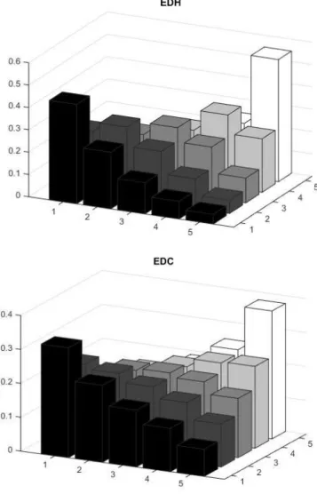
We investigate the persistence of systematic tail risk over time. We follow Chabi-Yo et al. (2018) by examining the relative frequency with which a stock belonging to quintile 𝑗 in a year moves to quintile 𝑖 in the next year. As argued by Chabi-Yo et al. (2018), if these frequencies are around 20 percent, then the risk measure in question is not persistent in the sense that past values of the measure contain little information about its future value. Figure 1 shows the relative frequencies of the EDH and EDC measures. It is clear that there is a high tendency for a stock belonging to a quintile in a year to stay in that quintile in the following year. The frequency of a stock staying in the same quintile is always more than 20 percent and considerably higher in some cases, particularly in the extremes. In quintile 5 (the highest level of exposure) and quintile 1 (the lowest level of exposure), the relative frequency with which a stock stays in these quintiles after a year is 54.67 percent and 44.49 percent for EDH
14
and 37.72 percent and 32.41 percent for EDC. These values are higher than the respective persistence values of the LTD measures in Chabi-Yo el al. (2018), where the frequencies for quintile 5 and quintile 1 are 31.61 percent and 26.60 percent. In unreported results, we also observe that the persistence of EDC and EDH is similar to, if not higher than, other risk measures such as downside beta, upside beta, coskewness, cokurtosis, among others.
[Figure 1]
5.2 Different Tail Risk Threshold Levels
In this section, we examine how altering the quantile level affects the performance of the systematic tail risk measures. Above, we use the five percent quantile of the return distribution for all measures. Table 4 reports results using both the 10 percent and one percent thresholds. The risk premium associated with both EDH and EDC measures is consistently significantly positive. By comparing this result with that of the five percent threshold in Table 3, we observe that the coefficient on EDC sharply reduces when the tail threshold is reduced from 10 percent to one percent, although it nevertheless remains highly significant. At very low tail thresholds, the EDC measure relies on a small number of observations. We observe that on average there are 5.29 co-exceedances between a stock and the market in a year at 10 percent tail threshold. The corresponding numbers of co-exceedances at the five percent and one percent threshold are 1.98 and 0.33, respectively. This highlights the tendency of individual stocks to exceed a threshold at the same time as the market, and this tendency increases the more extreme the threshold. Relative to the case of two independent variables, at the 10 percent, five percent and one percent thresholds, the expected number of co-exceedances in 250 days is 2.50, 0.63, and 0.03, respectively. However, this result also highlights the limitation of EDC measured at the very extreme tail as it relies on very few observations. Nevertheless, the significant tail risk premium corresponding to EDC implies the risk of co-exceeding an extreme threshold at the same time as the market is a concern for investors, regardless of how low that risk might be. The EDH measure does not suffer from this problem since we can obtain ETL for any significance level at the daily frequency. Therefore, the investigation using the EDH measure is reliable at any level of the tail threshold. Moreover, this feature of EDH also allows estimation using a short estimation window, which in turn enables us to examine below the impact of systematic tail risk on returns at very short horizons.
15
[Table 4] 5.3 Different Market Tail Risk Measures
We examine the robustness of the EDH measures by using different models for the daily market tail risk. We examine the performance of the EDH measure when the market ETL is estimated using GARCH, GJR GARCH and EGARCH models. Specifically, the GJR GARCH model in Equation (9) is replaced by the GARCH and EGARCH models in Equations (12) and (13) respectively:
𝜎𝑚,𝑡2 = 𝑐
0+ 𝑐1𝜎𝑚,𝑡−12 + 𝑐2𝜀𝑚,𝑡−12 (12)
𝑙𝑜𝑔(𝜎𝑚,𝑡2 ) = 𝑐0+ 𝑐1𝑙𝑜𝑔(𝜎𝑚,𝑡−12 ) + 𝑐2𝑧𝑚,𝑡−1+ 𝑐3[|𝑧𝑚,𝑡−1| − 𝐸(|𝑧𝑚,𝑡−1|)] (13)
where 𝑧𝑚,𝑡 is defined in Equation (7). We also allow the residual distribution to be either
Gaussian or Skewed Student-t. The details of the maximum likelihood estimation of these processes are available upon request. We also examine VaR instead of ETL as the daily tail risk measure for the market. The results with a five percent tail threshold are summarized in Table 5. We obtain similar results using the 10 percent and one percent tail risk measures.
[Table 5]
According to Table 5, all of the EDH measures have a consistently positive relationship with returns and are statistically significant. Thus, our results are robust to modification of the estimation model for market tail risk. Moreover, Table 5 also shows that sensitivity to ETL tends to have a larger impact than sensitivity to VaR. The coefficients of EDH based on ETL measures are always higher than those based on VaR using the same setting. The measures based on the Gaussian distribution reveal an important insight about the source of tail risk that is priced by investors, which we discuss in the next section.
5.4 EDH and Systematic Volatility Risk
The fat tails of the unconditional distribution of stock returns may be due to different sources: a time-varying conditional mean, time-varying conditional volatility and the non-normality of the conditional distribution. The impact of time-varying conditional mean and volatility is not trivial. In fact, even if the conditional distribution is Gaussian, time-varying mean and volatility can generate significant non-normality in the unconditional distribution. The literature contains many studies that successfully fit a mixture of Gaussian distributions or
16
regime-switching models to the empirical distribution of stock returns (see, for example, Kon, 1984; Billio and Pelizzon, 2000; among others).
These possible sources of tail risk raise an interesting question: which potential sources of fat tails are priced by investors. EDH can shed some light on this question. The EDH measure is based on the change in the daily tail risk of the market which can be decomposed into a change in the conditional mean, a change in the conditional volatility and a change in the conditional parameters of the standardized residual 𝑧𝑚,𝑡 in Equation (7).2 We do not specifically model the time-varying parameters of the standardized residuals in our framework. The change in the Skewed Student-t parameters from day 𝑡 − 1 to day 𝑡 is purely due to the change in the estimation sample, which is negligible. Thus, the change in market tail risk in our framework is induced largely by changes in the conditional mean and conditional volatility. To decompose the price impact of these factors, we estimate EDH along with Beta and systematic volatility using the framework of Ang et al. (2006b). Specifically, we regress the stock excess returns on the market excess return, the change in the Chicago Board Options Exchange’s VIX index3 and the change in the market ETL and obtain Beta (𝛽), systematic volatility (SV) and systematic tail risk EDH as coefficients:
𝑅𝑖,𝑡 = 𝑐𝑖+ 𝛽𝑖× 𝑅𝑚,𝑡 + 𝑆𝑉𝑖× ∆𝑉𝐼𝑋𝑡+ 𝐸𝐷𝐻𝑖 × ∆𝐸𝑇𝐿𝑚,𝑡 + 𝜀𝑖,𝑡 (14)
We further divide market excess returns 𝑅𝑚,𝑡 into 𝑅𝑚,𝑡+ and 𝑅𝑚,𝑡− which are equal 𝑅𝑚,𝑡 if 𝑅𝑚,𝑡
is higher and lower than its mean, and 0 otherwise, to estimate upside beta (𝛽+) and downside beta (𝛽−):
𝑅𝑖,𝑡 = 𝑐𝑖 + 𝛽𝑖−× 𝑅𝑚,𝑡− + 𝛽𝑖+× 𝑅𝑚,𝑡+ + 𝑆𝑉𝑖× ∆𝑉𝐼𝑋𝑡+ 𝐸𝐷𝐻𝑖× ∆𝐸𝑇𝐿𝑚,𝑡+ 𝜀𝑖,𝑡 (15)
We then use these estimated risk measures in our cross-sectional regression framework to investigate the corresponding risk premia. Thus, the risk premium of SV represents the price impact of the change in market conditional volatility. The risk premium of EDH now represents the price impact of the incremental information on tail risk above and beyond volatility due mainly to the change in the conditional mean as discussed above. Owing to the relatively short horizon of the VIX data, the sample covers the period from January 1986 to December 2017.
2 We would like to thank the referee for suggesting this analysis.
3 Similar to Ang et al (2006b), we use the old index VXO to expand the data back to January
17
Table 6 shows the result of this analysis and confirms the significance of both systematic volatility, as suggested by Ang et al. (2006b), and systematic tail risk. As expected, the systematic volatility risk premium has a negative sign since a stock with higher SV tends to offer higher returns when market volatility is high (a bad state of the market). This stock is more attractive to investors as it provides a hedge for volatility risk and, therefore, is sold at a higher price (lower expected returns). Importantly, the systematic tail risk premium is also significant and positive. Thus, systematic tail risk contains important information about asset returns, even after controlling for systematic volatility risk. This confirms that both sources of the fat tails of the return distribution (changes in conditional mean and changes in conditional volatility) are priced by investors. In fact, the robust performance of EDH based on the Gaussian distribution in the previous section supports this conclusion. Even when the standardized residual is normally distributed, the time-varying conditional mean and volatility can generate fat tails and both are priced by investors.
[Table 6] 5.5. Return Predictability of Systematic Tail Risk
In this section, we examine whether the systematic tail risk measures proposed in this study can be used as a predictive tool for future stock returns. To carry out this investigation, at the beginning of every month, we estimate the risk measures of the stocks in our sample using data over the previous 12 months and run the cross-sectional regression to predict the stock excess returns over the next month. We repeat this regression for every month in our sample and examine the time series average of the estimated coefficients. For the EDH measure, we use the expected EDH estimated from an autoregressive (AR) model using lagged EDH available in the previous month. Following Bali et al. (2009), we use an AR(4) model to estimate the expected EDH.4 We find that this approach performs better in predicting future returns than by using the raw lagged EDH value. This implies that investors take into account the evolution of tail risk over time. Similar to the cross-sectional regression in our standard framework, we apply weighted least squares in the cross-sectional regression of Asparouhova et al. (2010) to eliminate the microstructure effects.
[Table 7]
18
The first two columns of Table 7 show the predictability of the systematic tail risk measures estimated at five percent tail threshold relative to other canonical risk measures. EDC positively predicts next month’s return and the coefficient is highly significant. However, the coefficient of EDH is not significant. We investigate the reason for the weak predictive ability of EDH. We conjecture that it is due to the significant variation of EDH for stocks with very high or very low exposure. In unreported results, we find that the average EDH value of the top (bottom) 10 percentile of EDH in a year, although still the highest (lowest) average EDH value in the following year, decreases (increases) significantly. In the next two columns of Table 7, we run the predictive regressions excluding the stocks in the top 10 percent and bottom 10 percent of the cross-sectional distribution of the risk measures. The predictability coefficient of EDH reverts to the correct, positive sign.5 Thus, while EDH does not appear to have predictive power for returns for the whole cross-section of securities, it still has significant predictive power for a large portion of the stocks in the market. On the other hand, EDC has significant predictability regardless of the truncation of the sample and thus appears to be a universally effective predictor for future returns of stocks with different tail risk exposure.
5.6 The Tail Risk Premium over Different Horizons
One of the advantages of EDH is that it can be estimated with a very short sample and thus allows for the examination of how stock returns are affected by systematic tail risk at different horizons. In Table 8, we report the results of estimating the cross-sectional regressions where both the realized risk measures and the excess return on the left-hand side are estimated using one-month to twelve-month samples. The table reveals a monotonic increase in the tail risk premium when increasing the length of the sample period. Specifically, the premium of one-month tail risk is significantly negative. It becomes less negative for three-month EDH and turns to positive for six-month EDH. The premium is significantly positive for EDH estimated using a sample of at least nine months. In other words, stocks with high tail risk in a month tend to earn poor returns within that month. However, over a longer horizon, stocks with high tail risk tend to offer higher returns. This suggests that it takes time for investors to be compensated for bearing systematic tail risk.
5 In unreported results, we observe a monotonic increase in the significance of the
predictability of EDH when more stocks in the top percentiles are eliminated. The predictability of EDH becomes statistically significant if stocks in the top 30 percentile of EDH are removed.
19
When tail risk is high, the stock price should reduce so that its expected return increases to compensate investors for the higher risk. Therefore, over short horizons, we should observe a negative relationship between tail risk and returns, but the relationship should become positive at longer horizons when the compensation for high risk is realized. Our results suggest that the realization of the tail risk-return tradeoff takes about six months to materialize and becomes significant after nine months. Regarding the other risk factors, many of the risk-return relationships are consistent across different estimation windows, including downside beta, upside beta, book-to-market, reversal, illiquidity, volatility, and cokurtosis. However, size and coskewness have the opposite sign to that expected. This result suggests caution should be applied when basing short-term investment strategies on the established risk-return relationships. For example, investing in small capitalization stocks, despite being generally profitable in the long term, may well perform poorly in the short term. This finding is supported by Rachwalski and Wen (2016), who reach a similar conclusion.
[Table 8]
6. Conclusion
In this paper, we introduce two new systematic tail risk measures. The first captures the propensity of a joint crash between an asset and the stock market, while the second is based on the demand of investors to hedge against extreme downside risk. Using both measures, we find evidence of a significantly positive tail risk premium. The measures also have significant predictive power for future returns. One possible application for future research is to examine the pricing information in truly idiosyncratic tail risk. In addition to eliminating the canonical systematic risk factors such as market excess returns, size and book-to-market as in Huang et al. (2012), idiosyncratic tail risk should be also net of systematic tail risk. This could be done by filtering the systematic tail risk using the measures proposed in this paper. Owing to the fact that, in practice, investors are heterogeneous and not fully diversified, idiosyncratic tail risk should contain significant price-determining information, similar to that of idiosyncratic volatility (Fu, 2009; Rachwalski and Wen, 2016) and idiosyncratic skewness (Mitton and Vorkink, 2007; Boyer et al., 2010; Conrad et al., 2013).
20 References
Adrian, T., Brunnermeier, M.K., 2016. CoVaR. American Economic Review, 106, 1705-41. Alexander, C., 2009. Market Risk Analysis: Value at Risk Models. John Wiley & Sons. Alexander, G., Baptista, A., Yan, S., 2014. Banking Regulation and International Financial
Stability: A Case against the 2006 Basel Framework for Controlling Tail Risk in Trading Books. Journal of International Money and Finance 43, 107-130.
Amihud, Y., 2002. Illiquidity and stock returns: cross-section and time-series effects. Journal of Financial Markets 5, 31-56
Ang, A., Chen, J., 2002. Asymmetric correlations of equity portfolios. Journal of Financial Economics 63, 443-494
Ang, A., Chen, J., Yuhang, X., 2006a. Downside Risk. Review of Financial Studies 19, 1191-1239
Ang, A., Hodrick, R.J., Yuhang, X., Xiaoyan, Z., 2006b. The Cross-Section of Volatility and Expected Returns. The Journal of Finance 61, 259-299
Arditti, F., 1971. Another look at mutual fund performance. Journal of Financial and Quantitative Analysis 6, 909-912
Arditti, F., Levy, H., 1975. Portfolio efficiency analysis in three moments: the multiperiod case. The Journal of Finance 30, 797-809
Artzner, P., Delbaen, F., Eber, J.M., Heath, D., 1999. Coherent measures of risk. Mathematical Finance 9, 203-228
Asparouhova, E., Bessembinder, H., Kalcheva, I., 2010. Liquidity biases in asset pricing tests. Journal of Financial Economics 96, 215-237
Bali, T.G., Cakici, N., 2004. Value at Risk and Expected Stock Returns. Financial Analysts Journal 60, 57-73
Bali, T. G., Cakici, N., Whitelaw, R. F., 2014. Hybrid Tail Risk and Expected Stock Returns: When Does the Tail Wag the Dog?. Review of Asset Pricing Studies 4 (2), 206-246 Bali, T.G., Demirtas, K.O., Levy, H., 2009. Is There an Intertemporal Relation between
Downside Risk and Expected Returns? Journal of Financial and Quantitative Analysis 44, 883-909
Bali, T. G., Engle, R. F., Murray, S., 2016. Empirical asset pricing: the cross section of stock returns. John Wiley & Sons.
Barro, R.J., 2006. Rare disasters and asset markets in the twentieth century. Quarterly Journal of Economics 121, 823-866
Bawa, V. S., Lindenberg, E. B., 1977. Capital market equilibrium in a mean-lower partial moment framework. Journal of Finance Economics 5, 189-200
Billio, M., Pelizzon, L., 2000. Value-at-Risk: a multivariate switching regime approach. Journal of Empirical Finance 7, 531-554
Bollerslev, T., Todorov, V., 2011. Tails, Fears and Risk Premia. The Journal of Finance 66, 2165-2211
Boyer, B., Mitton, T., Vorkink, K., 2010. Expected Idiosyncratic Skewness. Review of Financial Studies 23, 169-202
Carhart, M.M., 1997. On persistence in mutual fund performance. The Journal of Finance 52, 57-82
Chabi-Yo, F., Ruenzi, S. and Weigert, F., 2018. Crash sensitivity and the cross-section of expected stock returns. Journal of Financial and Quantitative Analysis 53, 1059-1100 Chang, B., Christoffersen, P., Jacobs, K., 2013. Market skewness risk and the cross section of
21
Chiao, C., Hung, K., Srivastava, S., 2003. Taiwan stock market and four-moment asset pricing model. Journal of International Financial Markets, Institutions and Money 13, 355-381
Chung, Y.P., Johnson, H., Schill, M.J., 2006. Asset Pricing When Returns Are Nonnormal: Fama-French Factors versus Higher-Order Systematic Comoments. Journal of Business 79, 923-940
Conrad, J., Dittmar, R., Ghysels, E., 2013. Ex Ante Skewness and Expected Stock Returns. Journal of Finance 68, 85-124
Dittmar, R.F., 2002. Nonlinear Pricing Kernels, Kurtosis Preference and Evidence from the Cross Section of Equity Returns. The Journal of Finance 57, 369-403
Doan, P., Lin, C., Zurbruegg, R., 2010. Pricing assets with higher moments: Evidence from the Australian and US stock markets. Journal of International Financial Markets, Institutions and Money 20, 51-67
Fama, E.F., French, K.R., 1993. Common risk factors in the returns on stocks and bonds. Journal of Financial Economics 33, 3-56
Fama, E.F., MacBeth, J.D., 1973. Risk, Return and Equilibrium: Empirical Tests. Journal of Political Economy 81, 607
Fu, F., 2009. Idiosyncratic risk and the cross-section of expected stock returns.Journal of Financial Economics 91, 24-37
Gabaix, X., 2012. Variable Rare Disasters: An Exactly Solved Framework for Ten Puzzles in Macro-Finance. Quarterly Journal of Economics 127, 645-700
Geman, H., 1999. Learning about Risk: Some Lessons from Insurance. European Finance Review 2, 113-124
Gillman, M., Kejak, M., Pakos, M., 2015. Learning about Rare Disasters: Implications For Consumption and Asset Prices. Review of Finance 19, 1053-1104
Guidolin, M., Timmermann, A., 2008. International Asset Allocation under Regime Switching, Skew and Kurtosis Preferences. Review of Financial Studies 21, 889-935 Hansen, B., 1994. Autogregressive Conditional Density Estimation. International Economic
Review 35, 705-730
Harvey, C.R., Siddique, A., 2000. Conditional Skewness in Asset Pricing Tests. The Journal of Finance 55, 1263-1295
Huang, W., Liu, Q., Ghon Rhee, S., Wu, F., 2012. Extreme downside risk and expected stock returns. Journal of Banking and Finance 36, 1492-1502
Iqbal, J., Brooks, R., Galagedera, D., 2010. Testing Conditional Asset Pricing Models: An Emerging Market Perspective. Journal of International Money and Finance 29, 897-918
Kelly, B., Jiang, H., 2014. Tail risk and asset prices. Review of Financial Studies 27, 2841-2871
Kenourgios, D., Samitas, A., Paltalidis, N., 2011. Financial crises and stock market contagion in a multivariate time-varying asymmetric framework. Journal of International Financial Markets, Institutions and Money 21, 92-106
Kon, S. J., 1984. Models of Stock Returns – A Comparison. The Journal of Finance 39, 147-165
Kraus, A., Litzenberger, R.H., 1976. Skewness preference and the valuation of risk assets. The Journal of Finance 31, 1085-1100
Kuester, K., Mittnik, S., Paolella, M.S., 2006. Value-at-risk prediction: A comparison of alternative strategies. Journal of Financial Econometrics 4, 53-89
McNeil, A. J., Frey, R., 2000. Estimation of tail-related risk measures for heteroskedastic financial time series: an extreme value approach. Journal of Empirical Finance 7, 271-300
22
Meine, C., Supper, H., Weib, G., 2016. Is Tail Risk Priced in Credit Default Swap Premia. Review of Finance 20, 287-336
Mitton, T., Vorkink, K., 2007. Equilibrium Underdiversification and the Preference for Skewness. Review of Financial Studies 20, 1255-1288
Newey, W.K., West, K.D., 1987. A simple, positive semi-definite, heteroskedasticity and autocorrelation consistent covariance matrix. Econometrica 55, 703-708
Nieto, M. R., Ruiz, E., 2016. Frontiers in VaR forecasting and backtesting. International Journal of Forecasting 32, 475-501
Oordt, M., Zhou, C., 2016. Systematic Tail Risk. Journal of Financial and Quantitative Analysis 51, 685-705
Pástor, Ľ., Stambaugh, R.F., 2003. Liquidity Risk and Expected Stock Returns. Journal of Political Economy 111, 642-685
Rachwalski, M., Wen, Q., 2016. Idiosyncratic risk innovations and the idiosyncratic risk-return relation. Review of Asset Pricing Studies 6 (2), 303-328.
Rietz, T.A., 1988. The equity risk premium: a solution. Journal of Monetary Economics 22, 117-131
Wachter, J.A., 2013. Can Time-Varying Risk of Rare Disasters Explain Aggregate Stock Market Volatility? The Journal of Finance 68, 987-1035
Weigert, F., 2016. Crash aversion and the cross-section of expected stock returns worldwide. Review of Asset Pricing Studies 6 (1), 135-178.
23
Figure 1: Relative frequencies of the quintiles of tail risk measures.
This figure shows the relative frequency with which a stock belonging to quintile j moves into quintile i in the next year, averaged over the whole sample period from 1968 to 2017.
24
Table 1: Average excess returns of quintile portfolios sorting on systematic extreme downside risk measures
This table shows the average yearly excess returns and sizes of quintile portfolios sorted on different systematic extreme downside risk measures. The quintiles are sorted using 1 year realized risk measures contemporaneous to the quintile returns. The second row in each measure gives the value of the Newey-West t-statistics (in brackets) for the returns on the corresponding first row. The third row shows the average natural logarithm of the market capitalization of the stocks in each quintile. The last two columns are the average excess return of the long-short strategy which buys quintile 5 and sells quintile 1, and its alphas in Carhart (1997) four factor models. The overall sample period is from January 1968-December 2017. Quintiles 1 2 3 4 5 5 - 1 Carhart alpha EDH Average returns 13.063 12.215 13.662 15.133 22.254 9.191 7.883 t-statistics (5.159) (5.941) (6.032) (5.685) (5.232) (2.958) (2.047) Average size 18.128 19.024 19.393 19.617 19.605 EDC Average returns 10.645 10.878 13.993 17.181 21.599 10.955 8.491 t-statistics (4.341) (4.399) (5.473) (6.610) (6.601) (5.455) (4.169) Average size 18.216 18.755 19.115 19.465 20.105
25
Table 2: Average excess returns of quintile portfolios sorting on size and systematic extreme downside risk measures
This table shows the average yearly excess returns of 25 portfolios sorted on size and a systematic extreme downside risk measure. Size of a stock is the natural logarithm of its market capitalization at the sorting time. Systematic risk measure is the realized risk measures contemporaneous to the portfolio return. The second row in each size quintile gives the value of the Newey-West t-statistics (in brackets) for the returns on the corresponding first row. The last two columns are the average excess return of the long-short strategy which buys quintile 5 and sells quintile 1 of the systematic tail risk within each size quintile, and its alphas in Carhart (1997) four factor models. The overall sample period is from January 1968-December 2017. EDH Quintile 1 2 3 4 5 5 - 1 Carhart alpha Size Quintile 1 20.846 20.989 20.725 30.533 51.213 29.095 21.101 (6.316) (6.835) (7.063) (8.111) (8.095) (7.468) (6.736) 2 13.389 14.383 18.301 23.868 40.277 26.888 19.216 (4.457) (5.161) (5.848) (6.420) (6.696) (7.056) (5.809) 3 9.597 10.445 13.325 17.151 28.544 18.947 14.659 (4.169) (4.564) (4.441) (4.403) (4.653) (3.691) (2.842) 4 7.895 8.049 10.511 10.798 16.069 8.174 8.456 (4.201) (3.966) (4.789) (3.845) (3.657) (2.199) (1.717) 5 7.234 7.723 8.176 7.534 10.994 3.760 2.995 (4.524) (4.349) (4.695) (3.250) (2.983) (1.231) (0.809) EDC Quintile 1 2 3 4 5 5 - 1 Carhart alpha Size Quintile 1 19.878 20.019 25.164 28.344 39.492 19.614 18.239 (6.546) (5.998) (6.888) (8.094) (9.447) (9.417) (6.960) 2 12.796 13.266 17.894 23.663 32.157 19.361 12.771 (4.071) (3.930) (5.280) (6.093) (6.887) (6.205) (5.018) 3 4.655 8.319 13.722 17.966 25.370 20.715 17.518 (2.174) (3.034) (4.444) (5.459) (6.065) (7.513) (7.524) 4 2.306 5.338 8.929 14.001 21.206 18.900 15.968 (1.210) (2.233) (3.619) (5.529) (5.986) (7.130) (6.042) 5 0.114 4.659 8.051 12.569 15.357 15.243 14.164 (0.068) (2.394) (3.948) (5.238) (5.604) (7.074) (6.805)
26
Table 3: Cross-sectional analysis of systematic extreme downside risk
This table shows the Fama and MacBeth (1973) average risk premiums of canonical risk measures and of the proposed systematic tail risk measures, along with their corresponding Newey-West t-statistics (in brackets). In each cross-sectional regression, yearly excess return of a stock is regressed against its one year realized risk measures of downside beta and upsize beta (or CAPM beta), volatility, coskewness, cokurtosis and systematic tail risk; its lagged return, size, book-to-market, and illiquidity available at the time of the regression. The last column shows the cross-sectional mean and standard deviation of each independent variable in an average year of the overall sample period January 1968-December 2017.
Model I II III IV V VI VII Mean/Std
Intercept 0.109 1.013 0.544 0.543 0.614 0.633 0.639 1.000 (4.842) (7.560) (5.732) (5.813) (6.835) (6.488) (6.766) 0.000 𝜷− 0.097 0.104 0.062 0.067 0.038 0.955 (4.848) (5.557) (3.241) (3.552) (1.993) 0.633 𝜷+ -0.046 0.005 -0.032 -0.047 -0.033 0.813 (-6.094) (0.580) (-2.828) (-4.035) (-2.905) 0.687 𝜷 0.085 0.072 0.884 (2.271) (1.509) 0.525 Size -0.052 -0.034 -0.034 -0.037 -0.038 -0.037 19.357 (-7.684) (-7.303) (-7.408) (-8.004) (-7.801) (-7.864) 1.740 B/M 0.043 0.026 0.024 0.025 0.025 0.026 0.849 (5.248) (3.090) (2.917) (2.993) (2.981) (3.200) 0.604 Lagged -0.049 -0.046 -0.051 -0.052 -0.056 0.193 Return (-3.842) (-3.714) (-4.146) (-4.086) (-4.467) 0.448 Illiquidity 0.030 0.026 0.029 0.026 0.029 1.057 (11.808) (10.405) (10.652) (7.925) (9.485) 2.529 Volatility 2.716 2.946 1.960 1.464 0.878 0.026 (1.860) (2.068) (1.383) (0.904) (0.583) 0.011 Coskew -0.005 0.271 0.036 -0.016 -0.141 -0.095 (-0.100) (4.918) (0.757) (-0.459) (-3.130) 0.154 Cokurt 0.103 0.027 0.092 -0.003 0.069 1.905 (7.900) (2.006) (7.638) (-0.246) (6.235) 1.048 EDC 0.569 0.542 0.237 (11.227) (10.971) 0.145 EDH 0.028 0.019 1.645 (2.185) (1.715) 1.331
27
Table 4: Cross-sectional analysis of systematic extreme downside risk captured using different extreme downside thresholds
This table shows the Fama and MacBeth (1973) average risk premiums of canonical risk measures and of the proposed systematic tail risk measures estimated using different tail thresholds, along with their corresponding Newey-West t-statistics (in brackets). In each cross-sectional regression, yearly excess return of a stock is regressed against its one year realized risk measures of downside beta, upsize beta, volatility, coskewness, cokurtosis and systematic tail risk; its lagged return, size, book-to-market, and illiquidity available at the time of the regression. The sample period is from January 1968-December 2017.
Model 10 percent tail quantile 1 percent tail quantile
IV V IV V Intercept 0.535 0.611 0.534 0.619 (5.628) (6.793) (5.618) (6.907) 𝜷− 0.037 0.041 0.076 0.032 (2.102) (2.247) (4.064) (1.602) 𝜷+ -0.049 -0.033 -0.037 -0.036 (-4.390) (-2.798) (-3.120) (-3.177) Size -0.039 -0.037 -0.033 -0.037 (-8.047) (-7.985) (-6.948) (-8.046) B/M 0.023 0.025 0.025 0.025 (2.838) (3.006) (3.036) (2.975) Lagged -0.044 -0.052 -0.049 -0.051 Return (-3.664) (-4.135) (-3.796) (-4.150) Illiquidity 0.026 0.029 0.029 0.029 (10.540) (10.612) (11.246) (10.784) Volatility 3.727 2.028 2.493 1.847 (2.609) (1.419) (1.721) (1.315) Coskew 0.381 0.031 0.083 0.043 (7.097) (0.652) (1.741) (0.916) Cokurt -0.026 0.093 0.080 0.089 (-1.808) (7.650) (6.134) (7.576) EDC 1.042 0.146 (14.225) (9.354) EDH 0.023 0.040 (2.235) (2.214)
28
Table 5: Cross-sectional analysis of EDH measures captured using different models for market tail risk
This table shows the Fama and MacBeth (1973) average risk premiums of canonical risk measures and of the EDH measures estimated using different models for market tail risk, along with their corresponding Newey-West t-statistics (in brackets). In each cross-sectional regression, yearly excess return of a stock is regressed against its one year realized risk measures of downside beta, upsize beta, volatility, coskewness, cokurtosis and EDH; its lagged return, size, book-to-market, and illiquidity available at the time of the regression. The sample period is from January 1968-December 2017. The name of each regression model specifies whether the corresponding EDH measure utilizes market VaR or ETL, Gaussian or Skewed Student-t residual term distribution assumption, GARCH or EGARCHconditional volatility. Tail risk measure VaR GARCH Skewed t ETL GARCH Skewed t VaR GARCH Gaussian ETL GARCH Gaussian VaR EGARCH Skewed t ETL EGARCH Skewed t VaR EGARCH Gaussian ETL EGARCH Gaussian Intercept 0.601 0.600 0.600 0.600 0.612 0.615 0.612 0.614 (6.648) (6.666) (6.675) (6.679) (6.753) (6.791) (6.722) (6.732) 𝜷− 0.039 0.034 0.043 0.039 0.055 0.051 0.056 0.055 (2.295) (1.964) (2.381) (2.145) (3.070) (2.763) (3.301) (3.170) 𝜷+ -0.007 -0.003 -0.011 -0.008 -0.030 -0.032 -0.032 -0.032 (-0.477) (-0.231) (-0.821) (-0.580) (-2.742) (-2.963) (-2.836) (-2.870) Size -0.037 -0.036 -0.037 -0.037 -0.037 -0.037 -0.037 -0.037 (-8.089) (-8.082) (-8.113) (-8.105) (-8.032) (-8.050) (-8.027) (-8.032) B/M 0.025 0.025 0.026 0.026 0.025 0.025 0.025 0.025 (3.076) (3.074) (3.089) (3.092) (3.005) (2.994) (3.009) (3.002) Lagged -0.051 -0.051 -0.051 -0.051 -0.052 -0.052 -0.051 -0.051 Return (-4.158) (-4.171) (-4.150) (-4.162) (-4.144) (-4.149) (-4.103) (-4.118) Illiquidity 0.029 0.029 0.029 0.029 0.028 0.028 0.028 0.028 (11.349) (11.270) (11.566) (11.523) (9.930) (9.996) (9.913) (9.893) Volatility 2.346 2.274 2.366 2.327 2.362 2.299 2.393 2.375 (1.535) (1.495) (1.552) (1.532) (1.589) (1.547) (1.599) (1.582) Coskew 0.056 0.071 0.046 0.058 0.009 0.011 0.011 0.011 (1.086) (1.345) (0.953) (1.182) (0.195) (0.238) (0.243) (0.244) Cokurt 0.106 0.105 0.105 0.105 0.095 0.094 0.096 0.095 (8.210) (8.093) (7.983) (7.966) (8.029) (7.954) (8.112) (8.101) EDH 0.026 0.035 0.025 0.031 0.015 0.019 0.017 0.020 (4.341) (4.177) (3.897) (3.857) (1.761) (1.696) (2.013) (1.873)