Optimal Monetary Policy Rules under Inflation Range Targeting

(1)

This paper was written wile Medina and Valdés were affiliated with the Central Bank of Chile.

The authors thank Pablo García, Luis Oscar Herrera, and Felipe Morandé and seminar participants at the Central Bank of Chile for useful comments and accept responsibility for all remaining errors. This paper presents the views of the authors and does not necessarily represent in any way the positions or views of the Ministry of Finance, Chile.

1. This arrangement is part of a broader movement in monetary policy design in which the anchor of monetary policy is a target for inflation. See, for example, Bernanke and others (1999).

2. One reason for considering a deviation from a target range as being rela-tively more costly is its impact on credibility.

95

I

NFLATION

R

ANGE

T

ARGETING

Juan Pablo Medina

University of California, Los Angeles

Rodrigo O. Valdés

Ministry of Finance, Chile

Central banks resort to a variety of alternative arrangements in formulating, conducting, and communicating monetary policy. One increasingly popular type of arrangement is based on a target range for inflation.1_{In this setup the conduct of monetary policy is oriented}

to keeping inflation within preannounced boundaries. For example, the central banks of Brazil, Canada, Israel, New Zealand, and Swe-den all have target zones for inflation, whose width ranges from 2 to 3 percentage points. Chile recently announced an inflation target range of 2 to 4 percent, to begin in 2001. One can further distinguish two alternative arrangements for the target range, namely, soft-edged and hard-edged ranges. Under the former, deviations from the edges of the range are considered as adverse as a deviation from a point target, whereas in the latter, deviations from the target range are considered to be relatively more undesirable.2_{In other words, a}

soft-edged regime could be understood as a “thick” point target regime.

C

Monetary Policy: Rules and Transmission Mechanisms, edited by Norman Loayza and Klaus Schmidt-Hebbel, Santiago, Chile. 2002 Central Bank of Chile.

(2)

96 Juan Pablo Medina and Rodrigo O. Valdés Other central banks (for example, that of the United Kingdom and that of Chile until 2000) organize monetary policy around a point target, and some implicitly regard upward deviations of inflation as more costly than downward deviations. The latter is typically the case of a country trying to disinflate (examples include Brazil, Colom-bia, and Israel today and Chile during the 1990s).

In this paper we investigate how optimal monetary policy rules change under these alternative formulations. In particular, we com-pare optimal policy rules derived under alternative policy objectives or loss functions for a simple, backward-looking, dynamic model of the economy. We are interested in answering four related questions: First, does range targeting yield optimal monetary policy reactions that are less aggressive than otherwise?3_{Second, are there relevant}

nonlinearities for monetary policy under range targeting (for example, are there zones in which the optimal policy is inaction)? Third, what happens to optimal monetary policy reactions if the range edges are harder, that is, if deviations from the range are considered highly undesirable events? Finally, what are the implications of having an asymmetric objective, in which positive inflation deviations are rela-tively more undesirable than negative ones? Our purpose is not only to answer these questions but also to provide some quantitative mea-sures so as to evaluate their economic relevance. For that purpose we consider a simple but realistic model of the economy calibrated with Chilean data.

The economy for which we calculate optimal policy rules is ex-tremely simple, described by two linear equations: an accelerationist Phillips curve and an output gap equation. Monetary policy directly controls the real interest rate, which, in turn, affects output with a lag, and output affects inflation with another lag. For simplicity we consider neither any central bank preferences regarding interest rate variability nor any bounds for possible interest rate values. In gen-eral, the rules we derive will prescribe a more aggressive monetary policy than what a central bank would normally follow. Accordingly, rather than taking the quantitative results we derive at face value, they should be analyzed relative to the baseline scenario of rules for a symmetric point inflation target (derived from a standard quadratic loss function).

3. Other ways to make monetary policy less aggressive include the incorpora-tion of interest rate smoothness among the central bank’s objectives and the measurement of inflation over longer horizons (see, for example, Nessén, 1999).

(3)

This paper is closely related to the literature on optimal mon-etary policy rules developed by Svensson (2000), Ball (1999), McCallum (1998), and Woodford (1999), among many others. It departs from an otherwise standard analysis by comparing the implications of alter-native nonquadratic loss functions. It is closely related to Orphanides and Wieland (1999), who also study the effects of range targets for inflation. The key difference between that paper and this one is that Orphanides and Wieland consider no lags in the effects of the output gap on prices, whereas we model this effect as taking one period. In their model, monetary policy has a one-period control lag (that is, it affects inflation after one period), whereas in ours it has a two-period lag. Although this extra lag makes the model more realistic, it poses the difficulty of having a second state variable.4

The main results we find are the following: Compared with a qua-dratic loss function, range targeting yields a less aggressive optimal monetary policy. For example, after a 1-percentage-point inflation shock, interest rates increase by approximately one-third less when there is range targeting with soft edges than when there is point targeting. Optimal monetary policy in this setup is always active, however. That is, even if inflation is well inside the range, unless it is squarely in the middle of the target, interest rates should not be at their neutral level. Monetary policy moves in a preemptive way: be-cause the likelihood that a shock will move the economy out of the range increases when it is not in the middle of the range, it is optimal to move back the economy toward the center of the range. If range edges are relatively hard, range targeting implies a more aggressive monetary policy than when they are soft.5

If the loss function is the same as with point targeting, but with a discrete jump to zero in the inflation target range, optimal monetary policy does not change in any important way. If the loss function is asymmetric, penalizing positive inflation deviations more than nega-tive ones, optimal monetary policy involves higher average interest rates. This implies that this loss function generates (on average) a negative output gap.6

4. Orphanides and Wieland (1999) also include in their analysis a nonlinear Phillips curve and model uncertainty. We, in turn, focus our analysis on the impli-cations of having alternative loss functions.

5. Thus, there is an apparent trade-off between the width of the range and the form of its edges. The width generates less aggressive responses, whereas harder edges generate more aggressive responses.

6. A negative output gap is defined as one in which potential output exceeds actual output.

(4)

98 Juan Pablo Medina and Rodrigo O. Valdés The paper is organized as follows. Section 1 presents the basic model of the economy, discusses the procedure we use to transform a continuous economy into a discrete one, and reviews the dynamic programming framework we use to solve for the optimal policy rules. Section 2 compares the optimal policy rules derived under alterna-tive loss functions. Section 3 concludes.

1. G

ENERAL

F

RAMEWORK

This section presents the framework we use to calculate and com-pare optimal monetary policy rules under alternative loss functions. It describes the economy, the central bank’s preferences, and the method we use to find optimal monetary policy rules.

1.1 The Economy

We consider a simple, dynamic, backward-looking economy de-scribed by the following two equations:

, 1 1 - p - +a +e p = pt t yyt t and (1) , 1 1 r t yt t y t y r y =b _- +b _- +e (2)

where _p_t is the gap between inflation in period t and its long-run tar-get, y_t is the output gap, r_t is the real (or indexed) interest rate (mea-sured as a deviation with respect to its long-run level), and _AF

t and y t

A are (possibly correlated) serially uncorrelated mean-zero stochastic shocks. In the equations ay, br, and by are constant parameters.

These two equations are similar to those presented in Ball (1999) and Svensson (1997). Equation (1) is a standard accelerationist Phillips curve, and equation (2) is a standard output gap equation (a dynamic IS curve). Below we present an estimation of these equations using data for the Chilean economy. Notice that in this setup monetary policy has a two-period control lag over inflation.

At time t the central bank’s problem is to choose a sequence of interest rates

{ }

¥ = t t + 0 t

r so as to minimize the following expected intertemporal loss function:

(5)

x

, 0 úúû ù ê ê ë é d E =

å

¥ = t + t τ t t l L ₍₃₎

where _d is a discount factor, l(.) is an instantaneous loss function, and x_t is a vector of state variables x_t = (_p_t, y_t)'.

We seek to characterize the interest rate sequence through a time-invariant (and probably nonlinear) policy function for alterna-tive instantaneous loss functions. In particular, we seek to charac-terize and compare optimal policy (reaction) functions when the loss function is of the following type:

[

]

ï ï î ïï í ì ¥ p Î p + p -p p p Î p p ¥ -Î p + p -p = , for b c a , for b , for b c a 2 2 2 2 2 H t t H t H H L t t L t t L t L t y y y x l

where b, c, a_j and _F_j ( j = L, H) are constants.

This loss function includes the standard quadratic function with weights a and b in inflation and output gap variability, respectively. In this case pL =pH =0 and aL = aH. It also includes less standard setups such as target zones (for example, pL<0,pH >0, and c = 1)

and asymmetric weights (for example, a_L < a_H). Table 1 summarizes the five baseline cases we consider.7

Figures 1 and 2 show the alternative loss functions described in table 1. The quadratic case is meant to represent the standard point-target framework, whereas those with a zero value in the (_1, +1) range represent alternative range targeting setups. We also include an asymmetric objective function to represent higher costs of positive inflation deviations.8

In sum, the problem is to choose a sequence

{ }

¥ = t t + 0 t r that

mini-mizes equation (3) subject to equations (1) and (2). Under some regu-larity conditions, this problem has a solution that can be represented by a time-invariant policy function mapping the inflation and output gaps onto the real interest rate, r_t = h(x_t), where x_t is the vector of

7. Of course, one could also consider other parameters. Medina and Valdés (2002) considers the case of a one-sided objective.

8. Other asymmetries that may in general arise include asymmetric shocks and asymmetric responses of the economy.

(6)

Table 1. Parameter Values in Alternative Loss Functions

Loss function

Range with Range with Range with Asymmetric Parameter Definition Quadratic soft edges hard edges discrete edges “hawk” a_L Weight on downward inflation variability 1.0 1.0 1.25 or 4.0 1.0 0.5

a_H Weight on upward inflation variability 1.0 1.0 1.25 or 4.0 1.0 2.0

b Weight on output variability 0.5 0.5 0.5 0.5 0.5

c Weight on inflation variability inside the range 1.0 1.0 1.0 0.0 1.0

L

F Distance of lower bound of range from center 0 –1 –1 –1 0 (percentage points)

H

F Distance of upper bound of range from center 0 +1 +1 +1 0 (percentage points)

(7)

state variables (see, for example, Sargent and Ljungqvist, 1999). In this case x_t = (_p_t, y_t)'.

Unfortunately, for the class of loss functions we consider, it is not possible to find a closed-form solution for the function h(.). Only in the well-known case of a quadratic problem it is possible to find a vector F such that r_t = F

'

x_t yields the optimal solution. We there-fore have to resort to numerical methods. In particular, we change the original problem to one in which we constrain the states and control variables to be a discrete and finite set of points. We then apply standard dynamic programming techniques.9

9. Judd (1998) analyzes discrete-state space dynamic programming.

Figure 1. Loss Functions under Alternative Definitions of Range-Targeting

(8)

102 Juan Pablo Medina and Rodrigo O. Valdés 1.2 Discretization of the Continuous-State Space

We proceed as follows to transform the continuous economy de-scribed by equations (1) and (2) and the control variable r_t into a dis-crete-state space economy. We first assume that the economy can be in any of m possible states collected in a set _G = {(_p₁, y₁), (_p₂, y₂),…, (pm, ym)}. We further assume that the interest rate rt can take n different values arranged in a set _y = (r₁, r₂,…, r_n ).

To preserve the dynamic and stochastic properties embedded in equations (1) and (2), we calculate transition probabilities between states that depend on the interest rate. In this way monetary policy can be thought of as choosing alternative transition matrices of a Markov chain of the economy.

Assume that the shocks and y t

A follow a bivariate normal dis-tribution with variance-covariance matrix _S. It is then straightfor-ward to calculate the conditional distribution of the vector x_t = (pt, y_t)' conditional on (pt-1, yt-1) and rt-1 as the bivariate normal

distri-bution with mean of

and the following variance-covariance matrix:

, ,

.

Var x_t _p_t_-₁ y_t_-₁ r_t_-₁ ₌_å

To construct the transition matrix associated with each interest rate in _y, we divide a rectangle (a_F, b_F) _´ (a_y, b_y) _Í_Â2_into_m_equal-size

rectangles q1, q2,…, qm and consider that the centers of each of these rectangles form the set _G. For each feasible interest rate r_k_{Î y} we can define the transition probability p_{i j}k_{as the likelihood of a} move-ment from state (pi, yi) at time t _ 1 to state (pj, yj) one period ahead, given that r_t_₁ = r_k. This probability is given by

ò

´ q F F ú ú ú û ù ê ê ê ë é _- _S -S p ¸ ïþ ï ý ü ïî ï í ì ú ú ú û ù ê ê ê ë é _- _S -S p = y y j b a b a k i k i k i k i dx x x x x dx x x x x , , 1/2 2 / 1 , 2 ' exp 2 1 2 ' exp 2 1

_úûù êë é _p _Î_q _p ₌ _p ₌ = t t j t- t- i i t- k k ij y y y r r p Pr , ' ₁, ₁ , , ₁

(9)

where . , , E 1 1 1 ú ú û ù ê ê ë é = = p = p ÷÷ø ö ççè æ p = t_- i t_- i t_- k t t k i _y y y r r x

Armed with this set of transition matrices, we next find a solution of the original problem using standard dynamic programming. Clearly, because we consider a subset of the possible states of the economy, this discretization is only an approximation. Moreover, it should be clear that in the neighborhood of the borders of the rectangle (a_F, b_F) ´

(a_y, b_y) the approximation is far from accurate, for two reasons. One is that the probability of moving further away from the center of the rectangle is assumed to be zero, and the other is that the centers of the small rectangles _q_j at the borders do not properly represent the values that the system can take outside the (large) rectangle. When we calcu-late optimal policy rules, we use the complete rectangle, but we only consider the neighborhood of its center when we analyze and compare the implications of alternative loss functions.

1.3 Discrete-State Space Dynamic Programming With the economy represented in a discrete-state space, the original problem of the central bank becomes:

Min 0E ₀

,

, t t r y l t F @

å

¥ = t t ¥ = t t + subject to:

[

]

[

, , , , ,

]

, Pr , , , , , , , , , 1 1 1 1 1 1 1 1 k ij k t i i t t j j t t k t m m t t p r r y y y y r r r y y y = = p = p p = p = y Î p p = G Î p -+ + K K where

å

= = m j k ij p 1

1_{, for all}_i_{= 1,…,}_m_{and for all}_k_{= 1,…,}_n_. The Bellman equation associated with this problem is

,

_'

,

E

1, 1 ,

, ' , þ ý ü î í ì úû ù êë é _p _p d + p = p ₊ ₊ y Î l y V y y r min y V t t t t i i r t t (5)

(10)

104 Juan Pablo Medina and Rodrigo O. Valdés which, given the transition probabilities, can be written as

,

min

,

, 1 úû ù ê ë é p d + p = p

å

= y Î m j j j k ij i i r i i y l y p V y V k (6) for all i = 1,…, m and for all k = 1,…, n. Here V(pt, yt) is the optimal value of the objective function starting from an inflation _p_t and output gap y_t. The solution of the central bank’s problem is charac-terized by a value function V(.,.) that satisfies equation (6) and an associated policy function r' = h(p, y) mapping the state of the economy (_p, y) onto an optimal choice of interest rate. Since equa-tion (6) satisfies Blackwell’s sufficient condiequa-tions for a contracequa-tion (see Stockey and Lucas, 1989, p. 54), it has a unique solution V*_(.,.).

In cases in which the discrete-state space is small, it is not diffi-cult to solve the Bellman equation applying an iterative algorithm. Define v to be a vector in and T[.] to be an operator that maps vector v into a new vector T(v) = (tv₁, tv₂,…, tv_m) in which each ele-ment tv_i is given by

,

min , , , . 1 1 1 2 1 ÷÷ø ö ççè æ + p =

å

= = = m j m j j n ij m j j ij j ij i i i l y p v p v p v tv K ₍₇₎

Thus the Bellman equation can be represented by

, v T v=

which can be solved by iterating until convergence the following recursion:

[ ]

v . T v _s+₁ = _s

If is the value function of the problem, then the optimal policy function h satisfies

,

argmin . ' 1 ÷ ÷ ø ö ç ç è æ Î p =

å

= * m j j k ijv p y h r Ψ Î k r * v '

(11)

That is, for each pair (pt, yt), the function h yields the optimal interest rate r_t such that the central bank’s discounted intertemporal loss function is minimized.

2. C

OMPARISONOF

A

LTERNATIVE

L

OSS

F

UNCTIONS

This section calculates and compares optimal monetary policy rules for different loss functions using the methodology described above. In order to provide realistic results, it uses an estimation of the economy described by equations (1) and (2) using Chilean data. We then use the model presented above to calculate policy functions for alterna-tive objecalterna-tive functions and compare them against the standard qua-dratic loss function.

2.1 Estimation and Calibration

We estimate equations (1) and (2) using Chilean quarterly and semiannual data on core inflation and the output gap (calculated with a Hodrick-Prescott filter) from 1986 to 1998. Table 2 presents the basic results.10_{It also presents the values of the parameters that we}

finally use in the simulations. The interest rate is the short-term indexed rate that the Central Bank of Chile used for monetary policy during the period (the rate on its own ninety-day indexed securities in 1986-95 and the overnight interbank interest rate thereafter).

Although we broadly use the ordinary least-squares estimates for elasticities, we consider a lower innovation volatility in our simula-tions. In the case of inflation, the main reason for this assumption is that this variable displays significant ARCH (autoregressive condi-tional heteroskedasticity) effects. In fact, a standard ARCH-LM test on the equations in table 2 yields a p value of 0.06. Furthermore, as Magendzo (1998) has documented, this volatility has a positive and stable relationship with the inflation level. To verify this effect, we estimate the same equation (1) but use the ratio of actual to trend inflation instead of the value of actual inflation. The estimate still shows a significant effect of the output gap on changes in (relative)

10. We also considered in the estimation a one-period-lagged direct effect of interest rates on inflation. This was meant to capture the standard open-economy transmission mechanism from monetary policy to inflation through the exchange rate. The results, however, cannot be considered different from zero.

(12)

106 Juan Pablo Medina and Rodrigo O. Valdés

inflation. More important, the standard error of the innovations in this estimation is approximately 0.25. Considering this standard deviation and an annual trend inflation of around 3 percent, we calibrate the model using a quarterly standard deviation of 0.8 percent (for annualized infla-tion). For output we consider a standard deviation of 1.0 percent, to broadly take into account the effect of other known output determinants in Chile, such as conditions in the mining sector and fiscal policy. 2.2 Quadratic Preferences

To evaluate the accuracy of our discretization of the economy, we compare the optimal policy rules for a quadratic loss function that results from using the algorithm presented in the previous section with the results from a standard dynamic programming procedure using the continous-state space economy. For the lat-ter we use the standard linear regulator problem solution (see, for example, Sargent and Ljungqvist, 1999).

Table 2. Estimates of Parameters in Inflation and Output Gap Equations for Chile, 1986-98, and Values Chosen for Model Calibrationa

Parameter estimates

Parameter Using quarterly data Using semiannual data Calibration

Inflation (Phillips curve)

=y 0.49 0.54 0.50 (0.20) (0.16) I(_AF t) 0.030 0.011 0.008 2 R 0.08 0.43 Output gap >y 0.61 0.32 0.60 (0.07) (0.11) >r –0.43 –0.55 –0.50 (0.16) (0.32) I( ) 0.015 0.015 0.010 2 R 0.46 0.23 Correlation ( , y t A ) –0.05 0.21 0.00

Source: Authors’ calculations.

(13)

Notice that because output is not that persistent, monetary policy has to be quite active in order to affect inflation. We construct grids for inflation and output in the [_5, +5] range with increments of 0.25 and 0.5, respectively. We search for optimal interest rates in the [_17, +17] range with increments of 33 basis points at each point of the grid.11

Figure 3 presents the results of this exercise. The top left and top right panels show the optimal interest rate deviation for given devia-tions of inflation and the output gap, respectively. Each panel assumes

11. These grids imply that there are more than 58 million p_ik j's.

Figure 3. Optimal Policy Functions with a Quadratic Loss Function

Reaction to inflation deviation output gap deviation = 0

Reaction to output deviation inflation gap deviation = 0

Reaction to inflation deviation output gap deviation = 1 percent

Reaction to output deviation inflation gap deviation = 1 percent

(14)

108 Juan Pablo Medina and Rodrigo O. Valdés that the other variable has a deviation equal to zero. The bottom pan-els show the same functions but assume a positive (1 percent) devia-tion of the other variable. As mendevia-tioned above, the accuracy of the results is limited at the borders of the grid we consider. However, they are surprisingly accurate once we move away from these borders. In-deed, only in the policy response to extreme inflation deviations do the two reaction functions diverge. In what follows we present results us-ing deviations for the [_3, +3] range.

2.3 Range Targeting

Is monetary policy more or less aggressive with point or range targets? The answer obviously depends on how hard are the edges of the range under consideration. Figure 4 shows optimal policy reaction Figure 4. Optimal Policy Functions under Soft-Edged

Range Targeting

(15)

functions for a soft-edged target range with a 2-percentage-point width. To facilitate comparisons, it also presents the optimal reaction func-tions for a quadratic loss function. The soft-edged range is represented by a loss function with quadratic losses in the edges with the same parameters as in the quadratic case (see table 1 and figures 1 and 2 for details). It can be thought of as a “thick” point target.

The results show that, indeed, monetary policy is less aggressive with a range target with soft edges. For all practical purposes, the reaction functions are piecewise linear: when the inflation gap lies in the [_1.5, +1.5] range, the policy rule is a line with a slope 30 percent less steep than in the quadratic case. This means that monetary policy is one-third less aggressive when there is a target range. Outside the [_1.5, +1.5] range the monetary policy reaction function is still lin-ear, with a similar slope, but it starts at a higher level (in absolute value). The reaction function against output shocks is also piecewise linear. It is almost equal to the policy function in the quadratic case for gaps in the [_1.5, +1.5] range and less aggressive outside that range (by approximately 80 basis points). The magnitude of these differences is not large, but it is economically meaningful.

The results also show that monetary policy is always active. Even when an inflation shock leaves the economy well inside the target range, if it is not right at the middle of that range, interest rates should not be equal to their neutral level. The intuition behind this result is that monetary policy has to move in a preemptive way: be-cause new shocks are coming in the future, being close to the borders of the range is risky. Thus the central bank has to adjust interest rates in such a way that the economy moves closer to the middle of the target range.

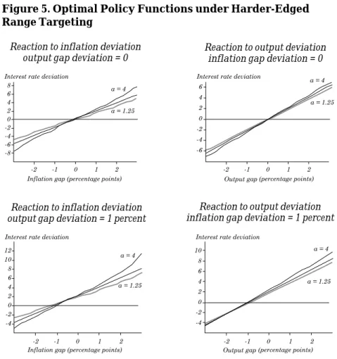
Figure 5 shows the results for two alternative cases in which the range edges are harder (a = 1.25 and a = 4). In these cases the opti-mal policy functions have some nonlinearities, although these are not substantial. When a = 1.25, that is, when a range deviation is considered 25 percent worse than a point deviation, optimal policy is still less aggressive with a target range than with a point target. When range deviations are considered four times as bad as point de-viations, policy is more aggressive. Numerically, following a 2-per-centage-point inflation shock, interest rates respond by approximately 10 percent more than in the quadratic case. When shocks are in the neighborhood of the target, differences are less important, and alter-native loss functions using the relatively harder edges yield similar outcomes.

(16)

110 Juan Pablo Medina and Rodrigo O. Valdés

Figure 5. Optimal Policy Functions under Harder-Edged Range Targeting

Reaction to inflation deviation

output gap deviation = 0 Reaction to output deviationinflation gap deviation = 0

Source: Authors’ calculations.

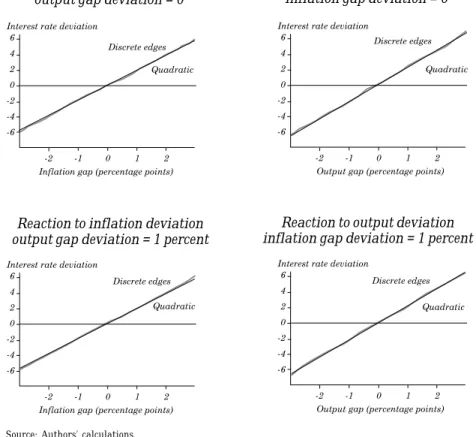
Figure 6 presents the case of a range with discontinuous edges, in which the loss function is the standard quadratic function that col-lapses (discontinuously) to zero inside the range (_1, +1). This could be thought of as a range that permits some limited flexibility, although outside the range, losses are the same as in the point target case. In other words, small deviations are not considered undesirable, whereas larger deviations are as costly as in the case of a quadratic loss func-tion. The result shows that from an economic point of view this range

(17)

does not yield any room for a less aggressive monetary policy. Indeed, the reaction functions in both cases are practically equal.

The intuition behind this result is simple. Because the economy is subject to continuous shocks, it is very unlikely that the economy will be very close to the middle of the range on a period-by-period basis. Therefore it is immaterial whether inflation deviations are considered neutral inside the target range. As a way to prevent movements out of this range, monetary policy has to be equally active.

Figure 6. Optimal Policy Functions with a Discrete Loss Function

(18)

112 Juan Pablo Medina and Rodrigo O. Valdés 2.4 Asymmetric Losses

If positive inflation deviations are considered more costly than nega-tive ones (for example, because of credibility problems or because the authorities are following a disinflation strategy), the loss function will be asymmetric, penalizing positive deviations more than negative ones. Figure 7 plots the policy functions for the case in which there is a point target but positive deviations are considered twice as costly as negative deviations (that is, a_L = 1, a_H = 2).

Figure 7. Optimal Policy Functions with an Asymmetric Loss Function

(19)

The result, as expected, is that monetary policy is, on average, tighter than in the quadratic (symmetric) case. Even when inflation is on target and the output gap is zero, interest rates have a positive bias. In general, reaction functions are still linear with respect to output deviations (although at a higher level), whereas they are clearly non-linear with respect to inflation, especially for large positive inflation deviations. When inflation is very low, the reaction function is parallel to that in the quadratic case (in this case, because a_L = 1, they are practically equal). But when inflation is positive, interest rates are increasingly higher in the former case.

Because interest rates are on average higher in the economy with asymmetric preferences, it is also the case that the output gap is, on average, smaller. That is, there is a bias against output.

3. C

ONCLUDING

R

EMARKS

This paper has investigated how optimal monetary policy rules change when the central bank considers alternative loss functions. In particular, it has evaluated the implications of considering a range target for inflation in a simple model calibrated to the Chil-ean economy.

The answers that this paper provides to the four questions posed in the introduction are the following. First, inflation range targeting indeed produces a less aggressive monetary policy re-sponse only when the range edges are not hard. If these edges are sufficiently hard, a range target involves more aggressive optimal monetary policy reactions. Specifically, a soft-edged range implies that interest rates move a third less than in the case of a point target. If the loss function is the same as in the case of a point target, but with losses equaling zero when inflation lies inside the target range, then optimal monetary policy does not change.

Second, there are some nonlinearities, but their economic rel-evance is not great. Interestingly, there are no inaction zones for monetary policy when there is range targeting. That is, monetary policy should always react to shocks, even if inflation is well inside the target range.

Third, if inflation deviations from the target range are consid-ered highly undesirable events__that is, if the target range has hard edges__optimal monetary policy will be more aggressive than in the

(20)

114 Juan Pablo Medina and Rodrigo O. Valdés case of a point target, in which deviations are always undesirable, but to a lesser extent. Therefore range targeting does not imply a less active monetary policy. The optimal policy will be more or less aggres-sive, depending on how hard the range edges are.

Finally, if positive inflation deviations are considered relatively more undesirable than negative ones, optimal monetary policy will be tighter than when the objective is symmetric. This means that in this environment the average output gap will be negative.

(21)

R

EFERENCES

Ball, L. 1999. “Policy Rules for Open Economies.” In Monetary Policy Rules, edited by J. Taylor. Chicago: University of Chicago Press. Bernanke, B., T. Laubach, F. Mishkin, and A. Posen. 1999. Inflation Targeting: Lessons from the International Experience. Princeton, N.J.: Princeton University Press.

Judd, K. 1998. Numerical Methods in Economics. Cambridge, Mass.: MIT Press.

Magendzo, I. 1998. “Inflación e Incertidumbre Inflacionaria en Chile.” Economía Chilena 1(1): 29-42.

Medina, J.P. and R. Valdés. 2002. “Optimal Monetary Policy Rules when the Current Account Matters”. In this volume.

McCallum, B. T. 1998. “Robustness Properties of a Rule for Monetary Policy.” Carnegie-Rochester Conference Series on Public Policy 29: 173-204.

Nessén, M. 1999. “Targeting Inflation over the Short, Medium, and Long Term.” Unpublished paper. Stockholm: Sveriges Riksbank (August).

Orphanides, A., and V. Wieland. 1999. “Inflation Zone Targeting.” Unpublished paper. Washington: Board of Governors of the Fed-eral Reserve System (June).

Sargent, T. J., and L. Ljungqvist. 1999. “Recursive Macroeconomic Theory."Unpublished paper. Stanford, Calif.: Stanford University. Stockey, N., and R. Lucas. 1989. Recursive Methods in Economic

Dynamics. Cambridge, Mass.: Harvard University Press.

Svensson, L. E. O. 1997. “Inflation Forecast Targeting: Implement-ing and MonitorImplement-ing Inflation Targets.” European Economic Re-view 41: 1111-46.

. 2000. “Open-Economy Inflation Targeting.” Journal of In-ternational Economics 50: 155-83.

Woodford, M. 1999. “Optimal Monetary Policy Inertia.” Working Pa-per 7261. Cambridge, Mass.: National Bureau of Economic Research.

(22)