On time series data and optimal parameters

(1)

Available online at www.sciencedirect.com

Omega 32 (2004) 111–120

www.elsevier.com/locate/dsw

On time series data and optimal parameters

Rasmus Rasmussen

∗

Institute of Economics, Molde University College, P.O. Box 2110, Molde 6402, Norway Received 18 June 2001;accepted 26 September 2003

Abstract

Forecasting using time series (TS) models are often based on linear regression or methods using various smoothing techniques. When estimating the parameters used in smoothing techniques, it has become a common practice to optimize the smoothing constants (parameters). This new practice is a result of the ease such methods can be accomplished when using the built in Solver optimization tool in modern spreadsheets. However, the capabilities of Solver can be utilized further to optimize more of the parameters, particularly the initial or starting parameters. This paper presents examples of exponential smoothing techniques, demonstrating improved /ts when adopting this idea of optimizing the initial parameters as well as the smoothing constants. It also demonstrates that linear regression is a special case of Holt’s exponential smoothing model with trend. Normalization of the seasonal parameters in models incorporating seasonality is also discussed, showing improved /ts to TS data. Educators are encouraged to adopt the idea of letting Solver optimize more of the parameters than what is common practice today, in other models and in other /elds.

Keywords:Forecasting;Time series;Regression;Spreadsheets;Education

1. Introduction

Forecasting using time series (TS) analysis is a frequently used quantitative technique when numbers concerning the future are required. Spreadsheets used on an electronic com-puter are becoming a common tool for managers and ana-lysts. Even though software specially designed for forecast-ing is available, the 7exibility and ease of use of spreadsheets combined with good graphing capabilities often makes them the choice of tools when performing the TS analysis [1].

Using spreadsheets to perform linear regression analysis or other models such as exponential smoothing techniques in TS analysis is becoming a standard in management science text books [2–5]. It is also becoming common practice to use Solver to choose the smoothing constant(s) [3, 5] for exponential smoothing techniques.

∗_{Corresponding author. Fax: +47-71-21-41-00.}

E-mail address:[email protected] (R. Rasmussen).

There are also add-ins to spreadsheets performing TS analysis, as CB Predictor, a tool that is a part of Crystal Ball Pro,1 _{and ForecastX.}2 _{How the smoothing constants and}

initial values are computed in these add-ins are not always disclosed in their manuals. A numerical example seems to indicate that only the smoothing constants are optimized.

In this paper I argue to go one step further, and also opti-mize the initial or starting parameters. These values are usu-ally estimated based on the /rst part of data in the TS. Often very simple formulas are used, as a shortcut to maintain the spreadsheet model simple. If the model includes seasonal adjustments, then normalization of the seasonal parameters often are skipped for the same reason.

The normalization of the seasonal adjustments is seldom mentioned in these introductory text books. For short-range forecasts skipping normalization will normally not make the forecasts go out of proportions, and long-range forecasts is usually not advisable based on these models. But skipping

1_{By Decisioneering;}_{http://www.decisioneering.com} 2_{By John Galt Solutions, Inc.;}_{http://forecastx.com}_.

(2)

112 R. Rasmussen / Omega 32 (2004) 111–120

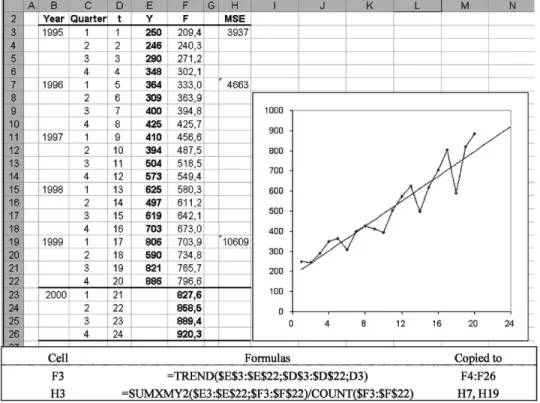
Fig. 1. Linear regression on a time series.

normalization may cause systematic forecasting errors com-pared to the theoretical model [6].

This paper therefore suggests utilizing Solver to simul-taneously optimize the smoothing constants and the initial values in the spreadsheet models forecasting TS data, when exponential smoothing methods are being used. With the in-creasing capabilities of Solver,3 _{educators are encouraged}

to adopt the idea of optimizing parameters normally treated as constants, also in other types of models. As such, this paper is heavily in7uenced by Ragsdale and Plane [1], ad-vising to simultaneously optimize the regression parameters and seasonal adjustments when regression models are used to forecast TS.

2. Models with trend

When a TS analysis with only trend is performed, a num-ber of models can be applied. This paper focuses on ex-ponential smoothing models, and illustrates Holt’s model compared to linear regression.

A linear regression model is easily implemented in a spreadsheet by using the built in TREND function to fore-cast a TS variable Yt (given historical data for the time

3_{Premium Solver Platform v3.5 is used in this paper. Frontline}

Systems;http://www.solver.com

periodst= 1;2;3; : : : ; n). Forecasts based on linear regres-sion are computed according to

Ft=b0+b1t; (1)

where the regression parametersb0andb1in (1) is estimated

by minimizing the mean square error (MSE): Min

b0;b1 : MSE (2)

and the MSE in (2) is de/ned as MSE = 1_n

n

t=1

(Yt−Ft)2: (3)

To reveal the parametersb0andb1the regression tool or

Solver can be used, but the TREND function in Excel is suf-/cient to make the forecasts directly. (Technically regres-sion is minimizing the sum of squared error (SSE), which equalsn×MSE.)

MSE for the complete series of data (t= 1;2;3; : : : ;20) for the linear regression model in Fig.1is 3937, which is the value minimized by the TREND function. Some models use /rst year for initialization, so forecasts can only be done fort= 5–20, and MSE for that period is therefore displayed for comparisons. MSE for the last cycle is also displayed, as this period often is regarded being most representative for the upcoming future.

Holt’s method is more 7exible than linear regression since it updates the level and trend parameters, which are constant

(3)

R. Rasmussen / Omega 32 (2004) 111–120 113

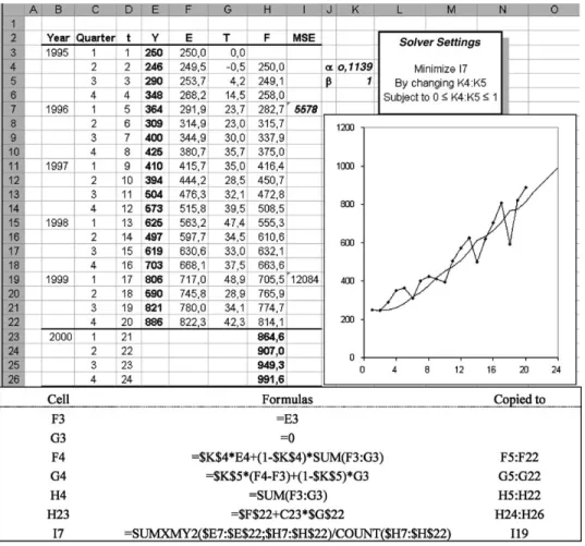
Fig. 2. Holt’s method with optimized smoothing parameters.

in linear regression. Forecasts at timetfor periodt+kare made by

Ft+k=Et+kTt: (4) The levelEt is updated as

Et=Yt+ (1−)[Et−1+Tt−1]: (5)

The trendTt is updated as:

Tt=(Et−Et−1) + (1−)Tt−1: (6)

Initial values have to be calculated to be able to update the values for level and trend. Several methods can be ap-plied, but to keep the formulas in the spreadsheet simple, the following formulas are sometimes used:

E1=Y1; (7)

T1= 0: (8)

The smoothing constantsandare parameters set within the limits 06, 61. Solver can be used to minimize MSE using one period forecasts (k= 1) for periods 2–20, but for comparisons the periods 5–20 is minimized.

The linear regression model in Fig.1has a better /t to the data (lower MSE) than the implementation of Holt’s method as shown in Fig.2. This is caused by how the initial values for level and trend are computed. Even though more sophisticated forms for Eqs. (7) and (8) can be applied, the initial values for level and trend should be part of the optimization model to get the best possible /t.

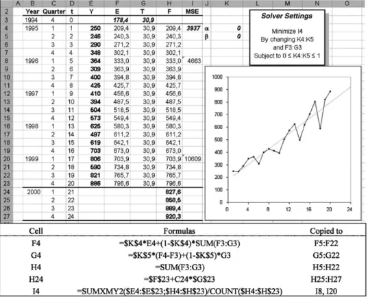
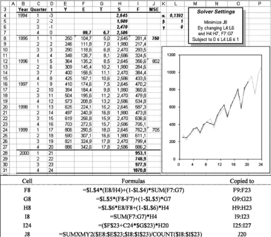
Implementing this modi/cation of the spreadsheet model, as in Fig.3, shows that if the optimal values for the smooth-ing constantsand= 0, thenE0=b0andT0=b1. In this case Holt’s model equals simple linear regression. This im-plementation of Holt’s model will never produce inferior /ts compared to linear regression. (The Solver model will have the same objective, but more decision variables, of which some applies to similar variables.)

3. Models with trend and seasons

Holt–Winter’s method adjusts for seasonal eLects, and can be applied with both additive and multiplicative seasonal

(4)

Fig. 3. Holt’s method with optimized smoothing parameters and initial values.

eLects. First the multiplicative version will be illustrated. In this model, forecasts are adjusted for seasonal eLects according to (9)

Ft+k= (Et+kTt)St+k−p: (9)

In Holt–Winter’s methodP equals the number of seasons per cycle (as 4 quarters per year). The updating procedure for the level is slightly modi/ed

Et= Yt St−p + (1−)[Et−1+Tt−1]: (10)

The trend is updated as before and repeated

Tt=(Et−Et−1) + (1−)Tt−1: (11)

The seasonal parameters are updated according to

St= Yt Et + (1−)St−p: (12)

To start updating the level, trend and seasonal parameters, we have to estimate initial values. Again there are several options. To preserve as much as possible of the data series for testing forecasts, a simple procedure of using only the

/rst cycle as initial period will be used.

St=₍₁_=pYtp t=1 Yt) fort= 1; : : : ; p; (13) Ep=Y_Sp p; (14) Tp= 0: (15)

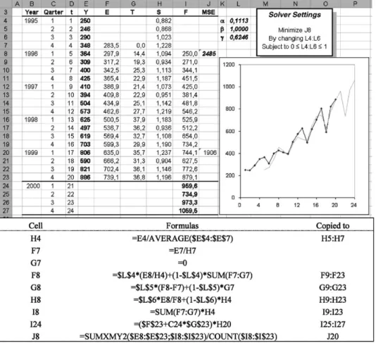
The smoothing constants; and are parameters set within the limits 06, , 61. Solver can be used to minimize MSE for the periods 5–20. This is implemented in Fig.4.

The TS data have obviously seasonal patterns, and the mod-el incorporating seasonal eLects makes a signi/cant improved /t to the data compared to previous models with only trend. However, we can improve the /t even further, by adopting the idea of optimizing the initial values for level, trend and seasonal parameters;in addition to optimizing the smoothing constants.

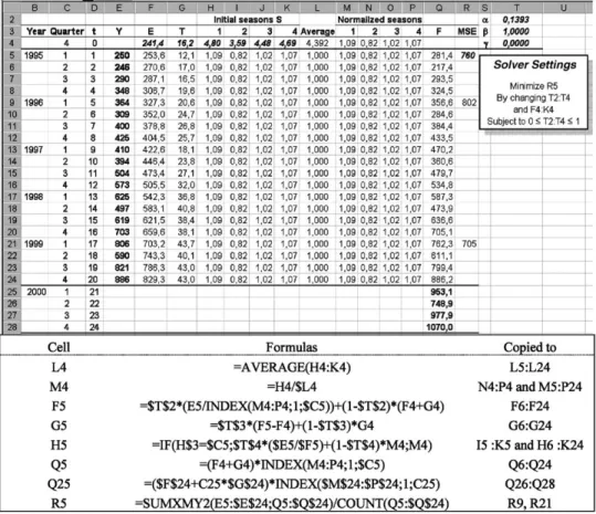
In Fig.5a new initial cycle is added, and Solver is set to optimize the starting values for level, trend and seasons as well as the smoothing constants,and. For TS with limited amounts of historical data, this technique can be valuable. We are now able to use all observations for testing purposes, not having to devote some part of the TS data for initialization.

(5)

Fig. 4. Holt–Winter’s multiplicative;with optimized smoothing parameters.

The MSE is signi/cantly reduced when both the initial parameters and smoothing constants are optimized, in this example MSE is improved for all compared periods. If there are reasons to believe that recent data is more representative for the expected future than older observations, Solver can be set to minimize MSE for the last cycle(s) instead of for the whole data set. Or the oldest and no longer representative parts of the data set can be deleted. Since we do not have to reserve data for initialization, the latter may be the most eMcient strategy.

4. Normalization

A note on normalization of the seasonal parameters should be made. As can be seen in Fig.5the sum of the initial sea-sons s−3+s−2+s−1+s0=9;631. This should theoretically

be equal P (4), or average to 1 for multiplicative models. If not, the model will make systematic forecasting errors [6]. Long-range forecasts can easily grow out of proportions. This is illustrated in the examples by the fact that this model is the one with the largest value for the latest forecast.

Normalization is usually skipped in introductory text-books, maybe for convenience, since the spreadsheet be-comes quite more complex. Normalization involves an iterative procedure in updating the seasonal parameters.

The averageA0must be computed before updating

At= 1_P t

i=t−p+1

Si: (16)

The normalized seasonal parameters for periods 0;−1; : : : ;−p−1 are then computed att= 0 as

Si ←_ASi

t fori=t; t−1; : : : ; t−p+ 1: (17) Then formulas (10)–(12), (16) and (17) are applied for updating att=1;2; : : : ; n. The normalization will assure that the seasonal parameters do not adopt changes in level or trend, only adjust to changes in the seasonal variations.

Again Solver is set to optimize the initial values for level, trend and seasons, along with the smoothing constants;

(6)

Fig. 5. Holt–Winter’s multiplicative;with optimized smoothing parameters and initial values.

The smoothing constants , and get the same opti-mal value as without noropti-malization, and the forecasts are identical with the model in Fig.5, where normalization is not performed. The only change from Fig.5is the values for the initial parameters. This occurs because the optimal smoothing constantfor the seasonal parameters is equal zero in this example. In that case the /rst normalization is suMcient, since the updated values will not change.

In the version with additive seasonal adjustments, the ad-vantage of normalization is more profound. The forecasts are changed as follows

Ft+k=Et+kTt+St+k−p: (18)

The updating procedure for the level, trend and seasons are slightly modi/ed

Et=(Yt−St−p) + (1−)[Et−1+Tt−1]; (19)

Tt=(Et−Et−1) + (1−)Tt−1; (20)

St=(Yt−Et) + (1−)St−p: (21)

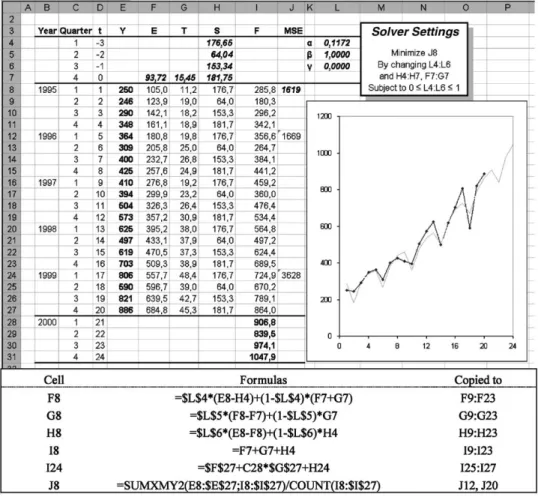
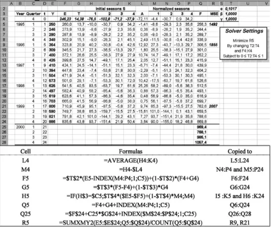
Solver is used to minimize MSE for the periods 1–20 by adjusting the smoothing constants,andwithin the limits 06,,61, as well as the initial parameter values for level, trend and seasons. This is implemented in Fig.7. The additive seasonal adjustments seem to not /t the data as well as the multiplicative adjustments. But to take full advantage of the model we again should normalize the sea-sonal adjustments. This implementation is done in Fig.8. The normalization in a model with additive adjustments of seasonal eLects is similar to the multiplicative model. In an additive model the sum of the seasonal parameters for a cy-cle (year) should equal 0. The normalization will assure that the seasonal parameters do not adopt changes in level or trend, but only adjust to changes in the seasonal variations. The average A0 is computed before updating as in (16). The normalized seasonal parameters for periods 0;−1; : : : ;−p−1 are then computed att= 0 as

Si ←Si−At fori=t; t−1; : : : ; t−p+ 1: (22) Thereafter formulas (19), (20), (21), (16) and (22) are ap-plied for updating att= 1;2; : : : ; n.

(7)

Fig. 6. Holt–Winter’s multiplicative;normalized optimized smoothing parameters and initial values.

An easy way to make the initial seasonal parameters is to add a constraint to Soiver. Make a constraint that cor-responds to A0= 0 for models with additive seasons or a

constraintA0= 1 for models with multiplicative seasons.

In Fig.7without normalization the average of the sea-sonal parameters is 144, indicating that some of the trend and level adjustments is adopted in the adjustments of the seasonal eLects. In Fig.8the normalization limits the sea-sonal adjustments to only capture seasea-sonal eLects, forcing the level and trend parameters to fully adopt these eLects.

The normalization has improved the /t as measured by MSE for the period being minimized (periods 1–20), and also for the last year isolated (periods 17–20). But MSE for periods 5–20 seems to be increased by normalization. How-ever, using Solver to minimize MSE for periods 5–20, then the MSE and forecasts are equal for both the non-normalized and the normalized version of the model with additive sea-sonal adjustments.

If MSE for the last year (periods 17–20) is being min-imized, both the model with multiplicative adjustments of seasonal eLects and the model with additive adjustments make perfect /ts to the data (MSE=0), both with and with-out normalization. (The models in Figs.5–8.) This

astonish-ingly good result is not a surprise when considering that the optimization model has 9 decision variables to /t the fore-casts for the 4 last quarters. But Solver superbly solves the complexity of the optimization problem. This perfect /t is not achieved without also optimizing the initial parameters (as the model in Fig.4).

The forecasting add-in tool CB Predictor selects Holt– Winter’s multiplicative method as the method being able to /t this TS data best. It does not /t the data as well as the optimized normalized version presented in Fig.6.

These examples indicate that normalization can help to improve the ability to /t forecasts to TS data.

5. Empirical tests

In these examples focus has been on /tting a forecasting model as close as possible to time series data. The ultimate test is of course to see how the forecasts /t the future, but these tests can only be done retrospectively. Therefore it is common practise to do “blind tests” by splitting the data in two series, the /rst part is used to /t the model to the data, and the recent part of the time series is used as

(8)

Fig. 7. Holt–Winter’s additive;with optimized smoothing parameters and initial values.

a hold out test, to see how accurate the model forecasts the “unknown” future. The model that most accurately de-scribes the holdout series is then selected for making the actual forecasts, after being re/t to the complete time se-ries. These previous examples may be regarded as this last step.

The rationale behind this practice is the belief that the model that most accurately prolonged its /tted pattern in the initial series into the holdout series also will be most accurate when prolonging the pattern from the complete data series into the real future. Just selecting the model that has the best /t to the complete time series may result in selecting a model that “over/ts” the data—incorporating random 7uctuations that do not repeat themselves.

And empirical tests seem to indicate that this is what is actually happening—statistically sophisticated models do not outperform simple forecasting techniques, the opposite may be the case [7].4 _{This fact has not stopped courses}

in advanced forecasting methods from being thought at the

4_{Particularly Chapter 11.}

universities or papers being published in journals. Instead emphasis is being made that forecasts should not rely on a single method, they should be made as a composite of several diLerent forecasting methods, also regarding quali-tative methods.

To test if the technique described in this paper over/ts the time series, a comparison to ARIMA models was done [8].5 _{The last year time series was used as holdout period.}

Two diLerent ARIMA models were developed, using Fore-castX. One model was developed by letting the software au-tomatically select an ARIMA model, the other model was completely speci/ed to the software. The speci/ed model had a slightly better /t to the initial data. ForecastX was also given the opportunity to freely select a forecasting model from its vast arsenal of techniques—this led to the selection of Holt–Winter with multiplicative season. MSE for these models are listed in Table2, following the models devel-oped after the guidelines in this article. Table1 lists the classi/cation of the exponential smoothing models used.

(9)

Fig. 8. Holt–Winter’s additive;normalized and optimized smoothing parameters and initial values.

Table 1

Pegel’s classi/cation Season

Trend None Additive Multiplicative

None A1 A2 A3

Additive B1 B2 B3

Multiplicative C1 C2 C3

Table 2

Using holdout data

MSE Initial Holdout

B2 Normalized 803,8 641,1 B3 Normalized 609,8 886,1 C2 Normalized 831,3 786,8 C3 Normalized 652,2 951,4 ARIMA(1,1,0) * (2,1,0) 771,9 1988,2 ARIMA(1,1,0) * (0,1,2) 719,0 1859,9 ForecastXB3 738,8 1287,5

The model that best /ts the initial series is Holt–Winter with additive trend and multiplicative season (B3). Based on the holdout series the selection is Holt–Winter with additive trend and additive season (B2).

We see that all models listed are making approximately equal good /t to the data seen by the model (MSE range from 610–830). The models made in accordance with this article have MSE in the holdout series comparable to the MSE in the initial series, two has lower and two has higher MSE in the holdout series. This is quite opposite to the more sophisticated statistical ARIMA models—both have more that twice as large MSE in the holdout series than in the initial series. We see that the Holt–Winter method applied by ForecastX (which does not normalize the seasons or ap-ply the technique of simultaneously optimize the smoothing constants and the initial parameter values);also make a con-siderable larger MSE in the holdout series than in the initial series.

This indicates that the recommendations made in this ar-ticle do not lead to over/t, comparing with the same model done the traditional way. The result is also in line with pre-vious empirical tests—more sophisticated (ARIMA) mod-els do not outperform simpler (exponentially smoothing) models. Compared to the sophisticated models there is no

(10)

120 R. Rasmussen / Omega 32 (2004) 111–120 indication that the methods described in this article will lead

to greater over/t, the opposite seem to be the case. 6. Optimization tools

The optimization models for minimizing MSE will be non-linear due to a non-linear objective function. But adding the initial parameters to the decision variables also will cre-ate non-linearity, since decision variables will be multiplied with each other.

With several decision variables in such complicated non-linear models, the optimization task will not be straight forward to solve. The standard Solver will /nd the nearest local optimal solution relative to the initial values of the decision variables set by the spreadsheet user. To search for alternative local optimal solutions will be like looking for a needle in a haystack. Fortunately, the Premium Solver Platform has a multistart search option, which has proven quite eMcient in these examples.

7. Conclusions

This paper outlines an approach whereby smoothingand initial parametersare found by solving directly the problem of minimizing MSE. The advantage is not only better /t to TS data. It will also reduce the need for data, since there will be no need to use data to estimate the initial parameters.

When initial parameters are optimized along with the smoothing constants, linear regression becomes a special case of Holt’s method.

The paper also advice to normalize seasonal adjustments in forecasting models. This extra complexity pays oL in better /ts and a theoretical sounder model.

References

[1] Ragsdale CT, Plane DR. On modeling time series data using spreadsheets. Omega 2000;28(2):215–21.

[2] Camm, JD, Evans JR, Management science and decision technology, 1st ed. Cincinnati, OH: Southwestern College Publishing;2000. p. 390.

[3] Ragsdale, CT. Spreadsheet modeling and decision analysis, 3rd ed. Cincinnati, OH: Southwestern College Publishing;2001. p. 794.

[4] Render B, Stair RM. Quantitative analysis for management, 7th ed. Englewood CliLs, NJ: Prentice-Hall;2000.

[5] Winston WL, Albright CS. Practical management science, 2nd ed. Paci/c Grove, CA: Duxbury;2001. p. 953.

[6] Mossin J. Operasjonsanalytiske emner. Oslo: Johan Grundt Tanum: 1972. 303 s.

[7] Makridakis, SG, Wheelwright SC, Hyndman RJ. Forecasting methods and applications, 3rd ed. New York: John Wiley & Sons Inc.;1998. p. 642.

[8] Hanke JE, Wichern DW, Reitsch AG. Business forecasting, 7th ed. Upper Saddle River, NJ: Prentice–Hall, Inc.;2001. p. 498.