Habit Persistence in Consumption in a Sticky Price Model of the Business Cycle
33
0
0
Full text
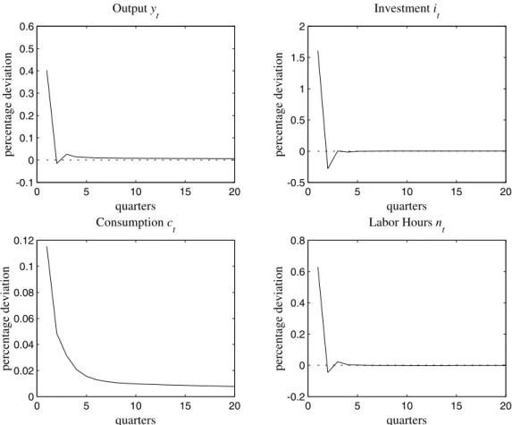
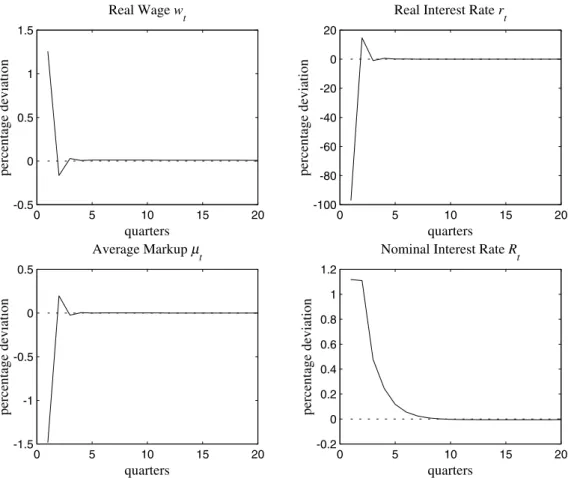
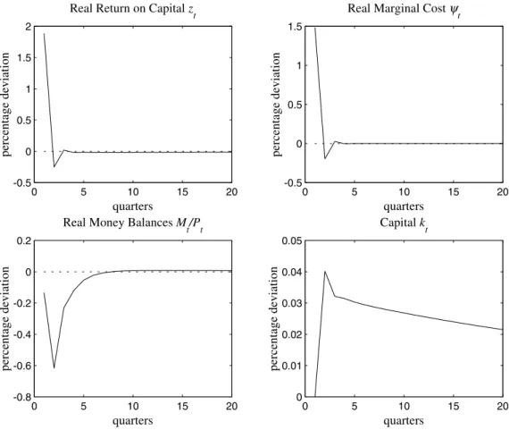
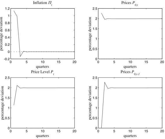
Figure
+3
Related documents