An Analysis of the 2008 Global Financial
Crisis: Was Quantitative Easing
Appropriate?
Naape, Baneng
University of Limpopo
15 December 2019
Online at
https://mpra.ub.uni-muenchen.de/97816/
Quantitative Easing Appropriate?
Baneng Naape
Department of Economics, University of Limpopo, South Africa Email: [email protected]
ABSTRACT: This essay aims to investigate the effects of Quantitative Easing (QE) on selected macroeconomic and financial market variables. By means of a desktop approach, we find that QE1 had a strong and beneficial impact on the real economy through the banking sector while QE2 and QE3 had small positive or neutral effects on banks and life Insurers. Although QE did not close the gap left by the 2008 global financial crisis, it helped reduce the rate at which the crisis was rising and proved to be an effective crisis management tool. QE boosts the economy in the short run but weakens the economy in the long run. Thus, central banks should only consider QE when the economy is in crisis and not as a substitution for structural reforms.
1. INTRODUCTION
As a result of the 2008 Global Financial Crisis (GFC) caused by subprime mortgages, central banks including the Bank of England (BoE), Bank of Japan (BoJ) and Federal Reserve, followed the unconventional monetary policy of purchasing large quantities of long-term securities to reduce long term interest rates, thereby spurring economic activity (Krishnamurthy & Jorgensen, 2011). This process is known as Quantitative Easing (QE).
Instead of printing new money, the central bank credits the sellers’ account which results in new electronic money. Notably, QE is considered when interest rates are at or approaching zero. The result of low interest rates has increased spending which raises the profits of non-financial firms. Furthermore, borrowing becomes less costly, resulting in business expansions and declines in unemployment rates which further leads to lower loan delinquencies and charge-off rates. All of these are necessary for a healthy economy and sound financial system (Chodorow-ReicH, 2014). Since 2009, the Federal Reserve has enacted two sets of QE both with different objectives.
The first and second rounds of the United States (US) QE began in December 2008 and November 2010 respectively, with the former aimed at increasing the avaliability of credit in private markets and the latter at strengthening the economic recovery and combating a possible Japanese-style deflationary outcome (Liber8 Newsletter, 2011). The European Central Bank (ECB) latter announced its own programme of QE in January 2015 (Oosthuizen, 2016). On the upside, QE has been empirically proven to have positive spill over effects. A recent study by Bhattarai and Chatterjee (2015) using a Bayesian VAR on monthly US macroeconomic and financial data, revealed that an expansionary policy results in an exchange rate appreciation, increased capital inflows, a stock market boom and reductions in long-term bond yields in Emerging Market Economies (EMEs). Against this backdrop, this essay aims to assess the effectiveness of QE enacted by various central banks
Page 1 of 12
since the 2008 GFC. This will be achieved by analysing trends in selected macroeconomic and financial market variables post QE announcements. The rest of the essay is arranged as follows: Section 2 provides a theoretical framework of QE, sections 3 and 4 detailing the effects of QE on macroeconomic and financial market variables, respectively. Finally, Section 5 details unwanted side effects of QE while Section 6 concludes the essay.
2. THEORETICAL FRAMEWORK OF QUANTITATIVE EASING
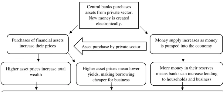
In this section, the process of QE is explained in detail. Below is a diagram illustrating how QE works and the various components and role players in the economy that are affected. Figure 1: Quantitative Easing explained
Source: Bank of England pamphlet (2011)
Central banks are often concerned with the risks of low inflation rates. As such, they usually reduce their lending rates so that borrowing becomes less costly to financial institutions and the public at large. Since interest rates cannot fall below zero, central banks inject new electronic money into the economy through the purchase of assets such as government bonds and high-quality debt from private companies (Liber8 Newsletter, 2011). The idea is not to print more banknotes but to credit the sellers bank accounts which results in new electronic money in the wider economy. The sellers will have more money in their bank accounts, while their banks will have a comparable claim against the central bank. The sellers, having more money, are then able to increase their spending, thereby boosting growth.
3. THE EFFECTS OF QE ON MACROECONOMIC VARIABLES 3.1.Inflation
QE is not without risks and chief among those risks is the risk of inflation. This is because, the amount of money in the economy is increasing but the quantity of goods for sale remains
Central banks purchases assets from private sector.
New money is created electronically.
Money supply increases as money is pumped into the economy Purchases of financial assets
increase their prices Asset purchase by private sector
More money in their reserves means banks can increase lending
to households and business Higher asset prices increase total
wealth
Higher asset prices mean lower yields, making borrowing
cheaper for business
Increased wealth and easier borrowing should encourage households and business to increase their spending
Increased spending should deplete inventories, which in turn should encourage business to employ more workers and raise income levels. This further increase spending, creating a virtuous circle.
Page 2 of 12
the same. In this instance, if production does not increase rapidly and the money does not exit the economy, inflation will result (Department of Finance Quarterly bulletin, 2011).
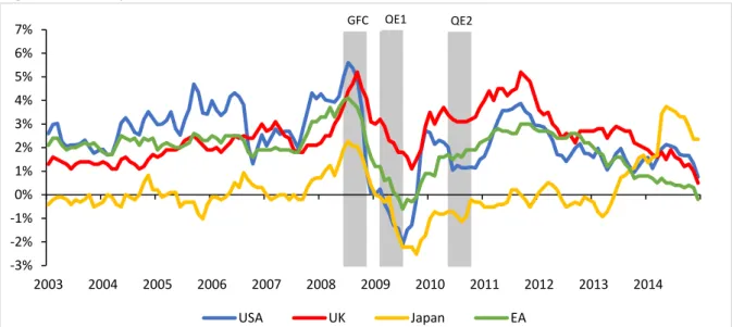
Figure 2: Monthly inflation rates
Source: author’s computations using OECD data (2016)
The US and United Kingdom (UK) through the BoE enacted their first rounds of QE in December 2008 (Chodorow-ReicH, 2014). In the Advanced Market Economies (AMEs), headline inflation fell below 1 per cent in February 2009, while core inflation ranged between 1½–2 per cent with the notable exception of Japan (World Economic Outlook, 2009). However, QE1 came to the rescue towards the end of 2009, pulling advanced countries out from deflation as business and consumer confidence rose. Nonetheless, headline inflation rates in AMEs recuperated in recent months (January – March 2017) as commodity prices bottomed out, although core inflation rates have remained widely unchanged and generally below inflation targets (World Economic Outlook, 2017). One of the goals of QE was to lower deflationary pressures in AMEs and this seems to have been achieved.
3.2. Commodity Prices
As substantial producers and exporters of commodities, EMEs are supposed to benefit from a commodity market recovery (Financial Stability Review, 209). For South Africa, QE resulted
in rising prices of precious metals such as gold (SA’s major export), platinum and Brent
Crude oil (Department of Finance Quarterly Bulletin, 2011).
3.2.1. Gold and Platinum
The price of Gold fell as a result of the GFC, reaching a trough of $713,5 per troy ounce, thereby increasing steadily in response to QE and reaching a peak of $1875,25 later in 2012 (SARB, 2017). This is beneficial to countries exporting gold as it improves their current account, though costly to those importing gold as they pay more money for the same quantity of the commodity. Most investors classified gold as a low risk commodity and can thus be reasonably assumed that money from QE moved into the gold market and increased the price
of one of South Africa’s major exports (Department of Finance Quarterly Bulletin, 2011). Trends in gold and platinum prices are illustrated in figure 3 below.
-3% -2% -1% 0% 1% 2% 3% 4% 5% 6% 7% 2003 2004 2005 2006 2007 2008 2009 2010 2011 2012 2013 2014 USA UK Japan EA GFC QE1 QE2
Page 3 of 12
Figure 3: Monthly gold and platinum prices
Source: author’s computations using South African Reserve Bank data (2017)
Persistent high gold prices had a positive effect on the fiscal revenue of gold-exporting countries while hindering gold-importing countries. The gold price rose steadily from $1201 per troy ounce in December 2014 to $1251 in January 2015 before declining gradually to $1131 in July 2015, showing little response to the Euro QE program.
3.2.2. Brent Crude Oil
For the importing country, a rise in the price of the commodity, more especially if the commodity is used in the production of other goods, can have serious adverse effects in the functioning of the entire economy. For example, a rise in the price of petrol will eventually lead to a rise in transportation costs, thereby increasing prices in general since transport costs are capitalised as production costs.
Figure 4: OPEC Brent crude oil price and output (monthly averages)
Source: author’s computations using Quandl data (2017)
The price of Brent crude oil fell to $33,73 per barrel in December 2008. Having fell sharply in 2008, the price rose by 62 per cent during the first half of 2009 (Financial Stability Review, 2009). Although the price of Brent crude oil continued to rise steadily towards the first quarter of 2010, the spot price declined by 9 per cent due to expectations of slower
0 500 1000 1500 2000 2500 U S ($) Gold Platinum 27 28 29 30 31 32 33 34 35 36 37 0 20 40 60 80 100 120 140 160 2003 2004 2005 2006 2007 2008 2009 2010 2011 2012 2013 2014 2015 2016 Mi lli o n s o f bar re ls p e r d ay US Do llars p e r b arr e l OUTPUT PRICE GFC QE1 € GFC QE1 QE1 € QE1 QE2 QE2
Page 4 of 12
global GDP growth and lower demand for commodities (Financial Stability Review, 2010). However, a weakening US dollar and positive investor sentiment have resulted in a rise in most commodity prices since July 2011. The spot price of Brent crude oil reached $110 a barrel in April 2011, compared to an average of $34 a barrel over the past 30 years (World Economic Outlook, 2011). Nonetheless, the price of crude oil increased in the first quarter of 2017, reflecting an agreement among major producers to trim supply (World Economic Outlook, 2017).
3.3. Real GDP
Vahey and Oppenheimer (2014) emphasized that the aim of QE is to lower long-term interest rates and lessen lending conditions. This will serve as an incentive for businesses to borrow money for capital expansion as borrowing costs will be lower (Oosthuizen, 2016). Subsequently, unemployment would decrease and national income and Gross Domestic Product (GDP) would rise.
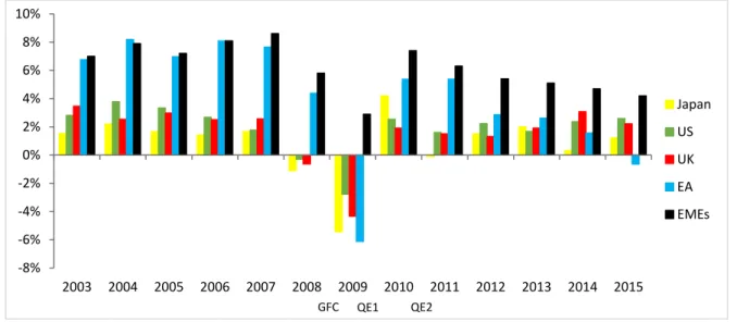
Figure 5: GDP growth (annual)
Source: author’s computations using World Bank and IMF data (2017)
The AMEs faced a downturn in economic activity during the period 2008 – 2009 as apparent from figure 5, experiencing an unparalleled 7,5 per cent decline in real GDP in the last four months of 2008 (World Economic Outlook, 2009). The recovery in economic activity gained momentum in the US and Japan in the fourth quarter of 2009, before moderating somewhat in the first half of 2010 (World Economic Outlook, 2010). In contrast, economic growth in the Euro Area (EA) and UK remained subdued in the first quarter of 2010 before accelerating strongly in the second quarter. World GDP at market exchange rates expanded 3,6 per cent in 2010, one year after an unprecedented contraction of 2,4 per cent that accompanied the financial turmoil in 2009 (World Trade Report, 2011).
3.4. Business sector
Following the global financial turmoil, global unemployment sharply increased to more than 210 million people, an increase of over 30 million since 2007. This had a huge negative impact on advanced economies, the aftermath being long-term social consequences, including on health and the children of those laid off (IMF News, 2010). Figure 6 shows trends in
-8% -6% -4% -2% 0% 2% 4% 6% 8% 10% 2003 2004 2005 2006 2007 2008 2009 2010 2011 2012 2013 2014 2015 Japan US UK EA EMEs GFC QE1 QE2
Page 5 of 12
unemployment rates while figure 7 shows trends in business and consumer confidence indexes for AMEs.
Figure 6: Annual unemployment rates Figure 7: Business and Consumer confidence
Source: World Bank data (2017) Source: OECD data (2017)
After the sharp rise in unemployment rates, the overall unemployment rate eased slightly in Japan, the US and UK in the first quarter of 2009. During this period, unemployment averaged 9,6 per cent in US, 7,9 per cent in UK and 5 per cent in Japan (World Bank, 2016). However, it continued to increase in the EA as apparent from Figure 6. According to the Financial Stability Review (2012), about 10 per cent of people of working age were unemployed in 2010. For developed economies, the unemployment rate decreased from 7,1 per cent in 2014 to 6,7 per cent in 2015 (International Labour Organisation Report, 2016). Notwithstanding, these improvements were not sufficient to close the jobs gap that evolved from the global financial turmoil. Unemployment rates for Japan, US and UK have been declining since 2010 and are expected to decline even further due to expected increases in output (World Economic Outlook, 2017). QE in this regard, reduced the rate at which unemployment rates were increasing. Nonetheless, business and consumer confidence responded positively to the first round of the US QE programme, although consumer confidence responded otherwise to the second round of the US QE programme. Business and consumer confidence in AMEs averaged 99,02 and 99,15 respectively in the second quarter of 2009 compared to 97,28 and 96,58 in 2008 (OECD, 2017). Notwithstanding, QE enacted by the BoE in early 2015 was not sufficient to boost overall business confidence in AMEs. Hence, the effects of QE on business and consumer confidence remain ambiguous.
3.5. Trade Patterns
The downturn in global economic activity became evident in the second half of 2008 and the first few months of 2009 as world trade flows and production deteriorated, first in AMEs and then in EMEs (World Trade report, 2009). Although global trade grew by 2 per cent in volume terms over the period 2008, it decreased gradually in the second half of the year and was well down on the 6 per cent volume increase recorded in 2007 (World Trade Report, 2009). Nonetheless, global output rose by 3,6 per cent in 2010 as merchandise exports surged
0% 2% 4% 6% 8% 10% 12% 14% 2000 2001 2002 2003 2004 2005 2006 2007 2008 2009 2010 2011 2012 2013 2014 US UK EA Japan 90 92 94 96 98 100 102 2004 2006 2008 2010 2012 2014 2016 BCI AV CCI AV
Page 6 of 12
to a record high of 14,5 per cent (World Trade Report, 2011). The trends in world trade volumes and prices are depicted in figures 8 and 9 below.
Figure 8: World trade volumes and prices Figure 9: Trade % of GDP
Source: CBP World Trade Monitor (2017) Source: World Bank data (2017)
World trade prices decreased substantially in the third quarter of 2008 from an average of $114 to a low $88,5 in the first quarter of 2009 (CBP, 2017). Apparently, China has become a leading manufacturer and exporter of manufactured goods in Asia, having achieved an average growth rate of 22,1 per cent (twice as fast as the world’s rate of 10 per cent) a year over 2002 – 2011 (SA Trade Report, 2014). Actual growth in world trade volume was 2,7 per cent in April 2016, revised from an estimate of 2,8 per cent (World Trade Report, 2016).
4. THE EFFECTS OF QE ON FINANCIAL MARKET VARIABLES 4.1. Interest rates
Central banks including the Fed, BoE and ECB, have reduced policy rates countless times since the sudden fall of Bear Stearns in March 2008 and have also purchased a combined US$12,3 trillions of assets over the period (2008 – 2015) according to Bank of America Merrill Lynch (Financial Stability Review, 2016).
Figure 10: short term nominal interest rates Figure 11: Gross capital formation
Source: OECD data (2017) Source: World bank data (2017)
40,0 50,0 60,0 70,0 80,0 90,0 100,0 110,0 120,0 130,0 2000 2001 2002 2003 2004 2005 2006 2007 2008 2009 2010 2011 2012 2013 2014 2015 2016 2016
World Trade Volumes World Trade Prices
0 20 40 60 80 100 2003 2004 2005 2006 2007 2008 2009 2010 2011 2012 2013 2014 2015 UK JPN US EA 0 1 2 3 4 5 6 2003 2004 2005 2006 2007 2008 2009 2010 2011 2012 2013 2014 2015 US Japan UK EA 0 10 20 30 40 50 60 70 80 90 2003 2004 2005 2006 2007 2008 2009 2010 2011 2012 2013 2014 2015 EA UK USA JAPAN
Page 7 of 12
As more money was pumped into the economy through the purchase of long-term government bonds and private sector assets, nominal interest rates across several countries including US, UK and EA fell from high rates of 5,9% in the last quarter of 2007 to low rates of 0,5% in the first half of 2009 (Department of Finance Quarterly Bulletin, 2011). Furthermore, to encourage credit institutions to extend credit to businesses and consumers in
order to revive the economy, the ECB’s lending to European credit institutions breached €1, 2 trillion in August 2012 (Financial Stability Review, 2012). However, long-term real interest rates have risen substantially since August 2016, particularly in the UK and US since the November election (World Economic Outlook, 2017). Nonetheless, gross capital formation in advanced market economies declined in 2008 and recovered in the first half of 2010 after reductions in interest rates.
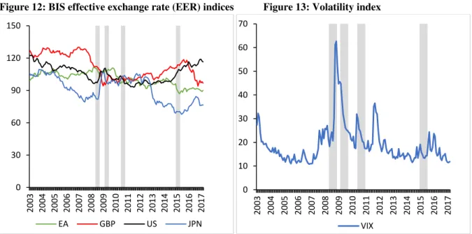
4.2. Exchange rates and Market volatility
Increased risk aversion brought about by the US sub-prime crisis of 2008 prompted a renewed focus on global disparities. Below are trends in exchange rates and volatility during QE dates. As can be seen in figure 13, QE resulted in massive volatility in the global market as the volatility index rose sharply from 20.7 per cent to 61.8 per cent in 2008 alone.
Figure 12: BIS effective exchange rate (EER) indices Figure 13: Volatility index
Source: Bank for International Settlements Source: Chicago Board Options Exchange (2017) The real effective exchange rate of the US dollar in April 2008 was about 25 per cent below its record high of February 2002 (Bank for International Settlements, 2009). The weakening trend in the exchange rate of the US dollar continued in the first half of 2008, deteriorating by 8 per cent against the euro and 5 per cent against the pound sterling (Financial Stability Review, 2008). However, the US dollar gained momentum in the second half of 2008, appreciating by about 6 per cent and 10 per cent against the euro and pound sterling respectively (Financial Stability Review, 2009). Notwithstanding, the Japanese yen
depreciated against its peers following the start of the Bank of Japan’s asset-buying programme (Financial Stability Review, 2013). General uncertainty and high levels of volatility in global financial markets were intensified by the US debt-ceiling discourse.
0 30 60 90 120 150 2003 2004 2005 2006 2007 2008 2009 2010 2011 2012 2013 2014 2015 2016 2017 EA GBP US JPN 0 10 20 30 40 50 60 70 2003 2004 2005 2006 2007 2008 2009 2010 2011 2012 2013 2014 2015 2016 2017 VIX
Page 8 of 12
4.3. Bond and equity markets
As a result of low interest rates and sufficient liquidity in most, if not all, advanced economies, QE has resulted in substantial capital flows into many EMEs over the period 2008-2015. This is mainly because, low interest rates in AMEs encourage investors to seek higher returns in EMEs where interest rates are relatively higher (Russell, 2016).
Source: Federal Reserve Bank of St. Louis Database (2017)
Figures 14 and 15 show changes in government 10yr bond yields and all share prices respectively for US, UK, Japan, Euro area and EMEs. The downward trend in government bond yields reversed in the first half of 2009 due to increased government borrowing. The reversal was related to brisk government expenditure alongside revenue which significantly undershot expectations (Financial Stability Review, 2009). The Morgan Stanley Capital International (MSCI) Emerging Markets Index fell by 37 per cent since the beginning of 2008, reflecting weaker equity and bond markets in many EMEs (Financial Stability Review, 2008). Nonetheless, from the low levels reached in March 2009, the All-Share Index (Alsi) at JSE increased by more than 50 per cent in the year to 31 August 2010 (Financial Stability Review, 2010). Against a backdrop of heightened financial market distress, global equity indices, on average, fell back early in the second quarter of 2012. Global equity markets rebounded towards the latter part of the second quarter of 2012, mostly reflecting hopes of further unconventional policy easing by major central banks.
5. LOOKING AHEAD
QE was critically important in breaking the downward trend caused by the 2008 global financial turmoil. However, most studies (i.e. Chodorow-Reich, 2014: IMF, 2013 and Financial Times, 2013) revealed that QE becomes more of a problem than a solution when it is used for a prolonged period. For example, Chodorow-Reich (2014) found that QE1 had a strong, beneficial impact on the real economy through the banking sector where as QE2 had small positive or neutral effects on banks and life Insurers. In addition, a Financial Report by Financial Times (2013) revealed QE to be having dilutive effects on asset prices overtime.
0 1 2 3 4 5 6 2006 2007 2008 2009 2010 2011 2012 2013 2014 2015
Figure 14: Long-Term (10 yr) Government Bond Yields (%) Including Benchmark, not seassonally
adjusted US UK EA JPN 0 0,5 1 1,5 2 2,5 2006 2007 2008 2009 2010 2011 2012 2013 2014 2015
Figure 15: Total share prices for all shares, monthly, Not seasonally adjusted
Page 9 of 12
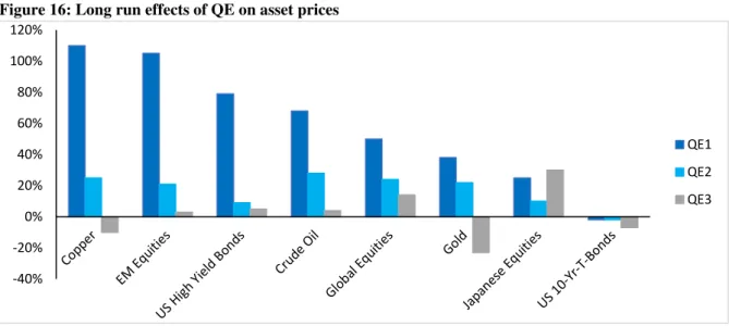
Figure 16 presents findings obtained from a Financial Times study on the impact of QE on asset prices.
Figure 16: Long run effects of QE on asset prices
Adapted from: Financial times (2013)
Although QE1 was successful in reviving asset prices as apparent from figure 16, QE2 produced less returns compared to QE1 while the returns from QE3 worsened. Sudeep (2010) argues that QE failed to restore economic growth in Japan. Jensen (2013) adds to the argument that, instead of reflating the global economy, QE in Europe and Japan is shrinking it. QE is well known for raising inflation expectations through the inflation channel, however, QE3 failed to raise inflation expectations in the US, argues the Washington DC (WashingtonsBlog, 2015). The longer the highly accommodative stance remains in place, the more probable its reactions are to develop (Jensen, 2013). A recent study by Chodorow-Reich (2014) in the US, revealed that the stock price index for life insurers changed by 1,96 percentage points in QE1; 1,29 percentage points in QE2 and 1,19 percentage points in QE3, reflecting diminishing returns. Furthermore, the study revealed that the stock price index for banks changed by 1,07 percentage points in QE1; 1,08 percentage points in QE2 and 0,76 percentage points in QE3.
Later US announcements, instead, had either more muted effects on all foreign assets (such as LSAP 3), or even negative effects on equities and bond yields (IMF, 2013). Although the returns may have been positive, they were increasing at a decreasing rate. Therefore, the following set of questions remains: Is QE still required after such an extended period, or should not central banks rather look at changing monetary policy approach? What about the role of fiscal policy side-by-side with monetary policy? Can the government also not look at structural challenges to the economy, thereby supporting monetary policy to deal with the problems that necessitated QE in the first place? For QE to be effective, banks must be willing to lend while firms and households must be willing to borrow.
6. CONCLUSION
From the above discussions, it is clear that unconventional monetary policies enacted by various central banks brought about their own benefits and costs. It is also clear that the short run benefits outweighed the costs. Most, if not all, objectives of QE were achieved. In the
-40% -20% 0% 20% 40% 60% 80% 100% 120% QE1 QE2 QE3
Page 10 of 12
short run, QE led to economic recovery and lowered deflationary pressures. The long-run costs of QE include, amongst others, inflationary pressures, slow growth and low saving rates. Although QE did not close the gap left by the global financial crisis, it helped reduce the rate at which the crisis was rising. Indeed, QE has proven to be an effective crisis management tool. However, because QE is used for an extended period, its side effects are emerging and deepening. QE boosts the economy in the short run but weakens the economy in the long run.
7. REFERENCE LIST
Bhattarai, S. & Chatterjee, A. (2015). Effects of US Quantitative Easing on Emerging Market Economies: University of Illinois
Bank of England pamphlet. (2011). Quantitative easing explained. Available at www.bankofengland.co.uk
Bhattarai, S. & Chatterjee, A. 2015. Effects of US Quantitative Easing on Emerging Market Economies. Federal Reserve Bank of Dallas: Globalization and Monetary Policy Institute, Working Paper No. 255
Chodorow-ReicH, G. (2014). Effects of Unconventional Monetary Policy on Financial Institutions. Brooking papers on economic activity: Harvard University
Department of finance Quarterly bulletin. Quantitative Easing and Its Effects on Economic Markets, April - June 2011
Lavigne, R. Sarker, S. & Vasishtha, G. (2014). Spill over Effects of Quantitative Easing on Emerging-Market Economies: International economic analysis
https://www.statbureau.org/en/japan/inflation-tables. Accessed on: 13 March 2017
http://www.federalreserve.gov/pubs/bulletin/2005/winter05_index.pdf. Accessed on: 15 March 2017
http://www.bankofengland.co.uk/boeapps/iadb/index.asp?Travel=NIxIRx&levels=2&XNotes =Y&A3951XNode3951.x=5&A3951XNode3951.y=1&Nodes=&SectionRequired=I&HideN ums=-1&ExtraInfo=true. Accessed on: 15 March 2017
International Trade Administration Commission of South Africa. (2014). South Africa trade report: Trade as a driver of structural change for sustainable development. Available at: www.itac.org.za/upload/ITAC%20AR%20-%2020%20August%20-%20Email.pdf
Krishnamurthy, A. & Vissing-jorgensen, A. 2011. The effects of Quantitative Easing on Interest Rates: Channels and Implications for Policy. North-western university
Liber8 newsletter. 2011. Quantitative Easing Explained: An informative and accessible economic essay with a classroom application. Available at: www.stlouisfed.org/education
South African Reserve Bank: Financial stability review. (2008 – 2016). Available at http://www.reservebank.co.za
Page 11 of 12
Vahey, J. & Oppenheimer, L. 2014. Last Call: The End of Quantitative Easing. Available: http://www.thirdway.org/report/last-call-the-end-of-quantitative-easing.
World Economic Outlook. (2017). An update of the key WOE projections. Washington DC World Trade Organisation. (2009 - 2015). World trade statistical review, available at www.wto.org/statistics
Oosthuizen, H. (2016). Policy Implications for South Africa as a result of Quantitative Easing and Monetary Policy Normalisation. Nedbank and Old mutual budget speech competition