NBER WORKING PAPER SERIES
INVESTMENT TAXES AND EQUITY RETURNS Clemens Sialm
Working Paper 12146
http://www.nber.org/papers/w12146
NATIONAL BUREAU OF ECONOMIC RESEARCH 1050 Massachusetts Avenue
Cambridge, MA 02138 March 2006
I thank Gene Amromin, Long Chen, Dhammika Dharmapala, Bob Dittmar, Ken French, Michelle Hanlon, Jim Hines, Li Jin, Marcin Kacperczyk, Gautam Kaul, Nellie Liang, Roni Michaely, Lubos Pastor, Monika Piazzesi, Jim Poterba, Steve Sharpe, John Shoven, Joel Slemrod, Moto Yogo, Lu Zheng, and seminar participants at the Federal Reserve Bank of New York, the University of Michigan, and Wharton for helpful comments and suggestions. I am grateful to Zhuo Wang for outstanding research assistance and to the Mitsui Life Center at the University of Michigan for financial support. The paper was previously circulated under the title “Tax Changes and Asset Pricing: Cross-Sectional Evidence." Address: Stephen M. Ross School of Business; University of Michigan; 701 Tappan Street; Ann Arbor, MI 48109-1234; Phone: (734) 764-3196; Fax: (734) 936-0274; E-mail: sialm@umich.edu. The views expressed herein are those of the author(s) and do not necessarily reflect the views of the National Bureau of Economic Research.
©2006 by Clemens Sialm. All rights reserved. Short sections of text, not to exceed two paragraphs, may be quoted without explicit permission provided that full credit, including © notice, is given to the source.
Investment Taxes and Equity Returns Clemens Sialm
NBER Working Paper No. 12146 March 2006
JEL No. G12, H20, E44
ABSTRACT
This paper investigates whether investors are compensated for the tax burden of equity securities. Effective tax rates on equity securities vary due to frequent tax reforms and due to persistent differences in propensities to pay dividends. The paper finds an economically and statistically significant relationship between risk-adjusted stock returns and effective personal tax rates using a new data set covering tax burdens on a cross-section of equity securities between 1927 and 2004. Consistent with tax capitalization, stocks facing higher effective tax rates tend to compensate taxable investors by generating higher before-tax returns.
Clemens Sialm
Stephen M. Ross Business School University of Michigan
701 Tappan Street
Ann Arbor, MI 48109-1234 and NBER
1
Introduction
If the marginal investor is subject to taxes, then before-tax asset returns should reflect the tax burden in equilibrium. In particular, assets facing higher tax burdens should offer higher risk-adjusted returns than less highly taxed assets. On the other hand, taxes should not be related to asset returns if the marginal investor is effectively tax-exempt, as first discussed by Miller and Scholes (1978). This study tests empirically whether before-tax equity returns are related to their effective tax rates using a new data set covering personal tax burdens on a cross-section of equity securities between 1927 and 2004.
McGrattan and Prescott (2005) derive the quantitative impact of tax and regu-latory changes on aggregate equity values using a growth theory model. They show that regulatory changes can explain the large secular movements in corporate equity values relative to GDP. McGrattan and Prescott (2005) base their inferences on a carefully calibrated growth model. However, they do not perform an econometric analysis of the relationship between tax rates and asset valuations and they do not investigate the cross-sectional implications of taxes.
My paper demonstrates that effective tax burdens vary substantially over time and cross-sectionally. Based on the average marginal tax rates derived by Poterba (1987b), I compute effective tax rates on equity securities. The aggregate tax bur-den on equity securities has declined over the last couple of decades as tax reforms reduced the statutory tax rates on dividends and capital gains. Furthermore, corpo-rations replaced a significant fraction of relatively highly taxed dividends with share repurchases. For example, effective tax rates on the market portfolio of common stocks exceeded 25 percent in 1950 and declined to less than 5 percent in 2004. In addition to the time-series variation in tax burdens, there is also a significant cross-sectional variation in tax burdens. Due to differences in the taxation of dividends
and capital gains, stocks that distribute a larger fraction of their total returns as div-idends tend to be taxed more heavily than stocks that distribute a smaller fraction of dividends. Dividend paying stocks faced, on average, an effective tax rate that is almost three times higher than the effective tax rate of non-dividend paying stocks.
The empirical test presented in this paper uses the time-series and the cross-sectional variation in tax burdens to determine whether the average returns of differ-ent equity securities depend on their tax burden. To obtain the effective tax burdens, I sort all publicly traded common stocks in the U.S. into portfolios according to the lagged annual dividend yield and compute effective tax rates on these portfolios. The results indicate that the average returns of these stock portfolios are positively related to their effective tax rates even after controlling for size, book-to-market, and mo-mentum effects. Adjusting for common factors in stock returns is important because dividend yields can capture risk effects (e.g., Fama and French (1992)) or mispricing due to behavioral biases (e.g., Lakonishok, Shleifer, and Vishny (1994)).
The impact of taxes on asset returns is economically and statistically significant. A one percentage point increase in the effective tax of an equity portfolio increases the average return of the portfolio by 1.54 percentage points after adjusting for the common factors of Carhart (1997). Numerous additional tests indicate that this relationship is robust over several sub-periods, using various measures of the effective tax rate, and using different econometric specifications.
Although the dividend yield is highly correlated with the effective tax rate, I demonstrate that the effective tax burden and not the dividend yield is the driv-ing force behind the higher expected returns. In particular, regressdriv-ing the abnormal Carhart returns on the dividend yield and on the interaction term between the div-idend yield and the divdiv-idend tax rate results in a significantly positive coefficient on the interaction term and in an insignificantly negative coefficient on the dividend yield. Thus, stocks paying high dividend yields tend to have relatively high
risk-adjusted returns particularly in periods when taxes are high. This result indicates that the reported effects are likely due to taxes and not due to the fact that dividend yields might proxy for additional risk or style effects not captured by the common factors of Carhart (1997).
These results are related to Fama and French (1998), who study whether the market value relative to the book value of a firm is related to dividends. Simple tax hypotheses would imply a negative relationship between dividends and relative asset valuations. However, they find the opposite result and infer that dividends convey information about the future profitability of a company, which is missed by a wide range of control variables. They argue that the information about the profitability obscures any tax effects of financing decisions. In my paper, I analyze the cross-sectional distribution of equity returns instead of relative valuation ratios.
The fact that taxes have an impact on asset returns implies that there are im-portant limits to arbitrage as discussed by Shleifer and Vishny (1997) and Fama and French (2005). There are several frictions that prevent investors to take advantage of the before-tax return differentials. First, tax arbitrage can cause trading costs that reduce the return of any strategy that generates high turnover. For example, a short-term dividend capturing strategy around ex-dividend days can cause significant trading costs due to the relatively small and frequent dividend payments. Second, significant risk remains in a long-term trading strategy that buys dividend paying stocks and shorts non-dividend paying stocks. The significant residual risk decreases the incentives for tax-neutral arbitrageurs to eliminate these price discrepancies.
Over the last several decades, the empirical effect of personal dividend and capital gains taxes on stock prices and stock returns has received a lot of attention in the
finance, economics, and accounting literatures.1 A first group of papers has analyzed
1See Auerbach (2002), Poterba (2002), and Allen and Michaely (2003) for reviews of this litera-ture.
whether asset returns depend on dividend yields, based on the after-tax version of the
CAPM by Brennan (1970).2 The results are sensitive to how dividends are measured
and whether some omitted risk factors that are correlated with dividend yields do explain the positive yield coefficient. In my paper, I compute the effective tax rates on different stock portfolios and relate the average returns on these portfolios directly to their tax burdens and not just to their dividend yields. By computing effective tax rates of equity securities, I take advantage of the substantial time-series variation in tax burdens of equity securities over the last eight decades.
A second group of papers analyzes the relationship between tax rates and
divi-dend yields using ex-dividivi-dend date price data.3 Elton and Gruber (1970) argue in
their seminal paper that stock prices should fall by less than the dividend if taxes affect investor’s choices, because dividends are taxed more heavily than capital gains. While the existence of a price drop on the ex-dividend day less than the dividend has been widely documented, it remains controversial whether this effect is due to taxes or alternative explanations, such as arbitrage by short-term traders or market microstructure. Analyzing long-term realized returns instead of ex-dividend day price behavior has the advantage that it is less susceptible to microstructure effects.
A third group of papers investigates directly whether there are capitalization
ef-fects around tax reforms.4 These studies generally find supporting evidence that tax
changes have an impact on asset valuations. However, event studies of tax reforms are plagued by several challenges. First, the events are often not easily identifiable due
2The papers in this literature include, for example, Black and Scholes (1974), Litzenberger and Ramaswamy (1979, 1980, 1982), Blume (1980), Gordon and Bradford (1980), Miller and Scholes (1982), Poterba and Summers (1984), Chen, Grundy, and Stambaugh (1990), Fama and French (1998), Naranjo, Nimalendran, and Ryngaert (1998), Dhaliwal, Li, and Trezevant (2003).
3The papers in this literature include, for example, Elton and Gruber (1970), Kalay (1982), Eades, Hess, and Kim (1984), Barclay (1987), Michaely (1991), Eades, Hess, and Kim (1994), Bali and Hite (1998), Frank and Jagannathan (1998), Green and Rydqvist (1999), Graham, Michaely, and Roberts (2003), Elton, Gruber, and Blake (2005), and Chetty, Rosenberg, and Saez (2005).
4The papers in this literature include, for example, Guenther (1994), Lang and Shackelford (2000), Ayers, Cloyd, and Robinson (2002), Sinai and Gyourko (2004), Amromin, Harrison, and Sharpe (2005), Auerbach and Hassett (2005).
to a multi-stage political process. It might take a relatively long time period from the initial proposal and the final enactment of the tax reforms. Second, many political decisions often are reversed relatively soon, resulting in relatively small capitalization effects if market participants recognize that these tax reforms are only temporary.
This substantial literature has not yet reached a consensus on whether dividend taxes are capitalized or not. My paper sheds light on this controversy by relating abnormal stock returns directly to effective tax burdens instead of investigating ex-dividend effects or particular events.
The paper is structured as follows: Section 2 derives the effective tax rates on various portfolios of equity securities. Section 3 reports the results of the empirical test investigating whether there is a relationship between average asset returns and effective tax rates, taking advantage of both the time-series and the cross-sectional variation in effective tax rates. Section 4 shows that the tax capitalization results are robust to numerous alternative specifications. Section 5 concludes.
2
Derivation of Effective Tax Rates
This section describes the derivation of the effective tax rate of equity securities be-tween 1927 and 2004. I compute the average tax rate faced by domestic taxable investors and investigate whether this measure of the aggregate tax burden is related to abnormal returns of equity securities. However, due to data limitations it is neces-sary to make several simplifying assumptions about the equity holdings of investors. In particular, it is not possible to observe the identify of the investors. This could potentially be problematic since clientele effects might induce highly taxed investors
to avoid high dividend yield stocks.5 Thus, the derived effective tax rate might be a
5For example, Allen, Bernardo, and Welch (2000) and Baker and Wurgler (2004) discuss why firms might pay dividends. Graham and Kumar (2006) Grinstein and Michaely (2006) are recent empirical studies of dividend clientele effects for individual and institutional investors.
noisy measure for the tax rate of the marginal investor. However, measurement error in the effective tax rate should bias the results against finding an impact of taxes on asset returns. I show in Section 4 that the tax capitalization results are robust using numerous alternative assumptions for computing effective tax rates.
2.1
Definition of the Effective Tax Rate
The effective tax rate of an equity security depends not only on the statutory tax rates but also on the management style of the stock portfolio. The tax burden on a stock portfolio can be reduced by holding assets with low dividend yields, by deferring the realization of capital gains, and by accelerating the realization of capital losses.
The expected effective tax yield of portfoliok at timet is given by:
ˆ
κk,t= ˆydivk,tτtdiv+ ˆyk,tscgτtscg + ˆyk,tlcgτk,tlcg. (1)
The expected effective tax yield depends first on the marginal tax rates on
divi-dends τdiv and short- and long-term capital gains τscg and τlcg, which are simply the
statutory marginal tax rates for specific income brackets.6
Furthermore, the composition of the sources of income from equity investments has an important impact on the tax burden of a portfolio. The expected dividend
yield ˆydiv is defined as the sum of the expected taxable dividends divided by the
initial value of the portfolio.7 Similarly, the expected short- and long-term capital
gains yields ˆyscg and ˆylcg are defined as the anticipated proportions of the portfolio
values that will be realized either as short- or long-term capital gains.8 The tax yield
6This section assumes that the statutory tax rates are known to investors at the beginning of each year. However, Section 4 shows that the empirical results are not affected qualitatively if the current tax rate is replaced by the lagged tax rate.
7Expected variables include a “hat” to distinguish between expected and actual variables. For example, ˆydiv
k,t denotes the expected or anticipated dividend yield of portfoliokduring yeart, whereas
ydiv
k,t denotes the actual realized dividend yield of portfolio kduring yeart.
ˆ
κk,t denotes the ratio between the total anticipated taxes and the current portfolio
value. The effective tax rate ˆτk,t is the ratio between the tax yield ˆκk,t and the
expected return of the portfolio.
To illustrate the various definitions, I report a simple example. Suppose that
the marginal tax rates on dividends and long-term capital gains are τdiv = 0.4 and
τlcg = 0.2 and that the expected dividend and capital gains yields are ˆydiv = 0.04 and
ˆ
ylcg = 0.02. In this case, the investor expects to pay taxes on dividends equal to 1.6
percent of the initial portfolio value (0.04×0.4) and taxes on long-term capital gains
equal to 0.4 percent of the initial portfolio value (0.02×0.2). Thus, the expected tax
yield ˆκ is 2 percent of the initial portfolio value and the expected effective tax rate ˆτ
is 20 percent using a 10 percent expected return.
2.2
Dividend and Capital Gains Tax Rates
Marginal statutory tax rates on dividend and long-term capital gains income have fluctuated considerably, as shown in Figure 1 and Table 1. The figure shows the statutory federal marginal dividend and long-term capital gains tax rates for house-holds in three different income brackets. Two income brackets correspond to real income levels of $100,000 and $250,000 expressed in 2004 consumer prices. The third bracket corresponds to the marginal tax rate for the top income bracket. Generally, dividend taxes are considerably higher and more volatile than long-term capital gains tax rates. The marginal short-term capital gains tax rates are not depicted separately since they are very similar to the marginal dividend tax rates. The construction of
due to the possibility to defer capital gains indefinitely. The deferral of the realization of capital gains is beneficial because the present value of the tax liabilities decreases if the tax payments are postponed. In addition, the taxation of capital gains can be avoided completely due to the “step-up of the cost basis” at the time of death, which eliminates the taxation of all unrealized capital gains. Constantinides (1983), Stiglitz (1983), and Constantinides (1984) describe several investment strategies to minimize the taxes of financial returns. Poterba (1987a), Auerbach, Burman, and Siegel (2000), Ivkovich, Poterba, and Weisbenner (2005), and Jin (2006) analyze the capital gains realization behavior of individual and institutional investors.
the time series is explained in more detail in Appendix A.1.9
To compute the average tax rates on dividends and capital gains, I follow Poterba
(1987b) and construct dollar-weighted average tax rates for dividendsτdiv and
short-and long-term capital gains τscg and τlcg. The Internal Revenue Service publishes
annually since 1917 the distribution of income sources of taxpayers in different income brackets. The marginal tax rate can be determined for each of these income brackets. The value-weighted mean of the marginal tax rates of investors in the different income brackets is called the “average marginal tax rate.” This tax rate will represent the average tax burden of investors in various tax brackets. Prior to 1965, I hand-collected tax distribution data from different issues of the Statistics of Income of the IRS. Since 1965, the NBER publishes the average marginal tax rates on an annual basis. Additional details on the construction of the dividend and capital gains tax rates are
summarized in Appendix A.2.10
Using the marginal tax rate of the average investor as the effective tax rate is consistent with the result of Fama and French (2005) that everyone’s portfolio choices contribute to expected returns in equilibrium if there are deviations from the standard CAPM assumptions. They provide a framework for studying how disagreement and tastes for assets as consumption goods can affect asset prices. Although they do not address the impact of taxes directly, tax distortions have a similar impact on asset prices as other market imperfections.
Figure 2 depicts the average marginal tax rates of dividend income and long-term capital gains between 1927 and 2004 based on IRS data for taxable investors. The average marginal tax rate on realized long-term capital gains is generally less than the average marginal dividend tax.
9The basic data set on statutory federal tax rates and on average marginal tax rates is identical to Sialm (2005). Sialm (2005) studies the time-series variation in effective tax burdens and aggregate valuation levels between 1917-2004 and does not investigate the cross-sectional impact of taxes.
10The data can be found at http://www.nber.org/ taxsim/dtdy/. Additional information on this microsimulation model can be found in Feenberg and Coutts (1993).
2.3
Dividends and Capital Gains Realizations
The sources of investment income for equity securities varied considerably between 1927 and 2004. Dividend income was the dominant source of income for stock hold-ers during most of the period. In the 1980s and 1990s, dividend yields decreased substantially as companies retained a larger proportion of their earnings and as they increased share repurchases. As a result of the dividend reductions, capital gains
became a relatively more important income source during the last two decades.11
The actual dividend yield of a stock portfolio ydiv
k,t is defined as the ratio between
the actual dividends paid during a 12-month time period divided by the initial price. Dividends are defined here as taxable dividends according to the CRSP distribution codes. The detailed codes are listed in Appendix A.5:
ydiv k,t =
dk,t
pk,t−1
. (2)
The annual Statistics of Income of the Internal Revenue Service report the ag-gregate short- and long-term capital gains and the dividends declared by individuals. The average propensities to realize short- and long-term capital gains are assumed
to equal the average propensities obtained from the IRS between 1927 and 2004.12
Furthermore, I assume that investors anticipate to realize a fixed proportion of capital
gains out of the expected returns net of expected dividend payments.13 Appendix A.3
explains the construction of the expected capital gains yields in more detail.
11See Fama and French (2001) for an investigation of the dividend paying behavior of U.S. com-panies.
12Between 1927 and 2004, the average aggregate short- and long-term capital gains yield based on IRS data are -0.11 percent and 2.05 percent, respectively.
13The assumption that only a fraction of the total capital gains are realized results in a lower effec-tive tax rate on capital gains, as discussed by Feldstein, Slemrod, and Yitzhaki (1980) and Poterba (1987a).
2.4
Dividend Portfolios
To obtain some cross-sectional variation in the effective tax burdens, the common domestic stocks in the CRSP database are divided into portfolios according to the lagged dividend yield and the lagged market capitalization of the companies. The portfolios are formed monthly for three sorting criteria. The first criterion forms 30 portfolios according to the dividend yield and the size of the underlying stocks. All the common stocks in the CRSP database are first sorted monthly into six groups based on their lagged one-year dividend yields (one group corresponds to non-dividend paying stocks and the other five groups correspond to quintile dividend yield portfolios). Subsequently, each of the six dividend yield groups is further divided into five quintile portfolios according to the lagged market capitalization. As commonly done in the asset pricing literature, the cutoff levels for the market capitalizations of the five quintile portfolios are based only on the distribution of the market capitalization on the NYSE. The second sorting criterion forms 11 portfolios based on the lagged one-year dividend yield. One of the 11 portfolios includes non-dividend paying stocks, and the other 10 portfolios are dividend yield decile portfolios. The third criterion forms two portfolios based on whether companies paid taxable dividends in the prior year. The portfolio returns are computed using value weights within each portfolio. However, the results do not differ much if I use equal weights instead, as explained in more detail in the empirical section.
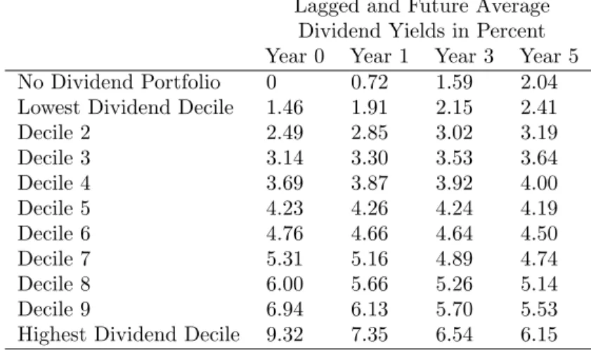
Table 2 shows the current and the future value-weighted dividend yields of the 11 dividend-yield portfolios. Although dividend yields revert towards the mean, dividend payments are relatively persistent. Thus, the tax properties of the 11 dividend yield portfolios do not tend to change dramatically over short time periods.
2.5
Anticipated Dividend Yield
The computation of the effective tax rate as described in equation (1) requires the
anticipated dividend yield ˆydiv, which is not observable. One possibility would be to
assume that the dividend yield follows a random walk. In this case, the anticipated dividend yield would be identical to the lagged actual dividend yield. However, this assumption would bias the results due to the mean reversion of the dividend yields as shown in Table 2.
To avoid any biases in the anticipated dividend yields, I estimate a partial
ad-justment model, where the actual dividend yield at time t of the stocks which are
included in portfolio k at time t−1 is regressed on the lagged dividend yield of the
same portfolio and on the lagged dividend yield of the market portfolio.
ydiv
k(t−1),t =αk+βkykdiv(t−1),t−1+γkyM,tdiv−1+²k,t. (3) This partial adjustment model allows for persistence in the dividend yield and for a reversion of the dividend yield toward the aggregate market yield. Since the composition of each portfolio changes slightly every year because of changes in lagged dividend yields and market capitalizations, it is important to follow the same set of underlying stocks over time. Thus, equation (3) relates the dividend yield of stocks
included in portfolio k at time t−1 with the dividend yield of the same portfolio of
stocksk(t−1) at time t.
Because of auto-correlated error terms and because of a lagged dependent variable, the coefficients of this linear model and the first-order auto-correlation are estimated using maximum likelihood. This partial adjustment model is estimated for each portfolio separately to allow the adjustment coefficients to differ depending on the dividend yield and the size of the stocks included in the portfolio. Furthermore, the estimation uses data at an annual frequency to avoid overlapping observations.
Table 3 summarizes the coefficient estimates for the partial adjustment model using 11 dividend yield portfolios. The auto-correlation term is important for no-dividend and low-no-dividend portfolios. The main determinant of the future no-dividend yield is the lagged dividend yield. The coefficient on the lagged dividend yield is often significantly smaller than one, indicating a relatively strong mean reversion effect. The fit of the model is relatively strong, as shown in the last column. The corresponding coefficients also are computed for the two alternative portfolio formation criteria based on 30 and two portfolios, respectively. I use the fitted values from this partial adjustment model to obtain an estimate of the anticipated dividend yield of portfolio
k during the next year ˆydiv
k,t.
2.6
Cross-Sectional Distribution of Effective Tax Rates
Based on these assumptions, it is possible to derive effective tax yields for differ-ent portfolios according to equation (1). Table 4 summarizes the momdiffer-ents of four different measures of the tax burden on equity portfolios using the three different portfolio formation criteria over the whole sample between 1927 and 2004. The first row in each panel summarizes the lagged value-weighted dividend yields. The sec-ond row summarizes the anticipated dividend yields based on the fitted value of the partial adjustment model according to equation (3). The last two rows summarize
the moments of the expected tax yield ˆκ and the expected effective tax rate ˆτ. The
effective tax rate ˆτ is simply defined as the ratio between the expected tax yield ˆκ
and the average return on all portfolios over the whole period. The moments of the different portfolio criteria differ slightly since they give different weights to different groups of stocks. For example, Panel C weights dividend and non-dividend paying stocks equally, which results in lower average tax burdens than Panel B, which gives relatively less weight to non-dividend paying stocks.
Figure 3 summarizes the variation of expected tax rates for the two value-weighted portfolios. The first portfolio includes all stocks that do not pay any taxable dividends and the second portfolio includes all other stocks. The effective tax rate of dividend paying stocks is substantially larger and more volatile than the effective tax rate of non-dividend paying stocks. The difference in tax burdens is particularly pronounced in the 1940s and 1950s and in the late 1970s. On average, dividend paying stocks face taxes that are almost three times higher than non-dividend paying stocks.
3
Taxes and Asset Returns
This section presents the main test of the capitalization of personal taxes taking advantage of both the time-series and the cross-sectional variation in tax rates.
3.1
Empirical Specification
The empirical estimation of the tax effects on equity returns is done in the base case in two stages. In a first stage, abnormal asset returns are computed based on con-ventional factor pricing models, such as the one-factor CAPM, the three-factor Fama
and French (1993) model, and the four-factor Carhart (1997) model.14 The empirical
specification of the Carhart model is as follows:
rk,t−rF,t = α+βk,tM(rM,t−rF,t) +βk,tSM B(rS,t−rB,t)
+βHM L
k,t (rH,t−rL,t) +βk,tU M D(rU,t−rD,t) +²k,t. (4)
The return of portfolio k during time period t is denoted by rk,t. The subscript
M corresponds to the market portfolio and the subscript F to the risk-free rate.
14The results are not affected significantly if I introduce in addition to the Carhart factors the liquidity factor according to Pastor and Stambaugh (2003). The liquidity factor cannot be used over the whole sample period since it is only available between 1966-2004.
Portfolios of small and large stocks are denoted by S andB; portfolios of stocks with high and low ratios between their book values and their market values are denoted by
H and L; and portfolios of stocks with relatively large and small returns during the
previous year are denoted byU and D. The Carhart model nests the CAPM model,
which includes only the market factor, and the Fama-French model, which includes the size and the book-to-market factors in addition to the market factor.
The factor loadings β denote the sensitivities of the returns of a portfolio to the
various factors. The factor loadings are estimated during a rolling window using data on the previous 60 months. This rolling factor regression reduces the length of the sample of abnormal returns by five years.
To determine the abnormal return ˜αk,t at time t of portfolio k, I subtract the
expected portfolio return based on the previously estimated factor loadings from the expected excess portfolio return:
˜
αk,t = rk,t−rF,t−βk,tM−1(rM,t−rF,t)−βk,tSM B−1(rS,t−rB,t)
−βHM L
k,t−1(rH,t−rL,t)−βk,tU M D−1(rU,t−rD,t). (5)
In a second stage, the abnormal return is regressed on the tax yield ˆκ:
˜
αk,t =γ+δˆκk,t+²k,t. (6)
The coefficient δ should be positive if investors are compensated for the personal
taxes by obtaining higher before-tax returns for assets facing higher tax burdens, particularly in periods where taxes are relatively high. A coefficient of one implies that the abnormal return increases exactly by the amount of the tax. However, the coefficient can differ from one because the marginal investor might differ from the average investor used to compute the effective tax yield and because of general
equilibrium effects.15
The two-stage estimation method ensures that the dividend yield coefficient does not capture risk effects that are included in the Carhart factors. However, the two-stage methodology might bias against finding an impact of taxes on asset returns, because some factors in the first-stage regression might proxy for the tax burden of the different portfolios. For example, the market or the size factors might be related to the dividend yield since small and high-beta stocks are less likely to pay dividends. As a robustness test, I also report in Section 4.5 a one-stage regression that estimates
the tax yield coefficient δ simultaneously with the factor loadings.
The estimation of the impact of taxes on asset returns is related to the speci-fications of Brennan (1970), Litzenberger and Ramaswamy (1979, 1980, 1982), and Naranjo, Nimalendran, and Ryngaert (1998). The earlier papers use the CAPM model as the relevant factor model while Naranjo, Nimalendran, and Ryngaert (1998) base their inferences on the Fama-French model. My estimation differs from the previ-ous papers by taking into account both the cross-sectional variation in tax burdens (different dividend yields) and the time-series variation in tax burdens (changing tax regimes). In addition, my estimation includes a momentum factor and covers a longer time period than the previous papers. While Naranjo, Nimalendran, and Ryngaert (1998) cover the period between 1963 and 1994, my estimation covers the period between 1927 and 2004, a time period that includes many large tax regime changes.
15Sialm (2005) derives in a general equilibrium model the impact of taxes on asset prices and asset returns if taxes are stochastic. In this model, asset returns increase more than the amount of taxes if investors are more risk-averse than log-utility investors. This is caused by the fact that sufficiently risk-averse investors need to be over-compensated for taxes, because they have a desire to smooth consumption over time.
3.2
Dividend Portfolios
Figure 4 depicts the rolling coefficient estimates of the factor loadings based on the Carhart model for the returns of value-weighted portfolios of dividend paying and non-dividend paying stocks between 1932 and 2004. Since the non-dividend portfolio accounts for a large fraction of the total market capitalization during most of the sample period, it is not surprising that the market beta is very close to one and that the other factors do not differ much from zero. However, there is an interesting variation in the estimated factor loadings of the non-dividend portfolio. The results indicate that non-dividend paying stocks tend to have a higher exposure to the aggregate market and they tend to be smaller stocks. Furthermore, non-dividend paying stocks tend to be value stocks before 1960 and they tend to be growth stocks after 1980. Non-dividend paying stocks in the early part often were distressed companies with relatively low market values, while non-dividend paying stocks in the latter part were often young companies with favorable growth prospects. Due to this significant variation in the factor loadings, it is crucial to estimate time-varying factor loadings. Table 5 summarizes the raw and the abnormal returns of the portfolios formed according to the lagged dividend yield. The table lists the averages of the time-series of these monthly excess and abnormal returns using the rolling regression methodol-ogy as summarized in equation (4). The first column reports the raw returns between 1927-2004, and the other columns report the abnormal returns between 1932-2004.
Table 5 demonstrates that stocks paying high dividend yields tend to have signif-icantly higher average abnormal returns than stocks paying no or low dividend yields using the CAPM, the Fama-French, and the Carhart factor models. For example, stocks in the highest dividend decile outperform non-dividend paying stocks by 38
basis points per month after adjusting for the four-factor Carhart model.16
16The fact that asset returns of high-dividend stocks tend to be relatively high seems at first glance to contradict the catering theory of dividends of Baker and Wurgler (2004), which argues
The return differences are slightly less pronounced if the portfolios are equally weighted instead. The Carhart abnormal return difference between the top dividend decile and non-dividend paying stocks amounts to 28 basis points per month, but remains statistically significant at a one percent confidence level. These results are consistent with the hypothesis that investors require higher expected returns for high-dividend stocks because of their higher tax burden.
3.3
Average Abnormal Returns and Tax Yields
Figure 5 depicts the relationship between average annualized abnormal returns and the average annualized tax yield for the 30 dividend/size portfolios over the sample period between 1932 and 2004. For each of the 30 portfolios, I compute the average excess return over the market. In addition, I compute the abnormal returns for the one-, three-, and four-factor models using rolling regressions as summarized in equation (5). The figures show a positive relationship between average tax yields and average equity returns regardless of the risk-adjustment method. This result shows that there is a robust relationship between tax yields and risk-adjusted asset returns even after aggregating all observations over time and ignoring the time-series variation in tax burdens. The relationship is weaker using excess market returns. This occurs primarily because of the very high excess return for the portfolio that includes non-dividend paying stocks that are in the smallest market-capitalization quintile. These stocks have the lowest effective tax rates and the highest average excess returns. The high abnormal performance of these stocks is reduced after adjusting the returns for common factors in stock returns.
that managers pay dividends when investors put a stock price premium on payers. However, the evidence of Baker and Wurgler (2004) is primarily based on the aggregate time-series variation of corporate payout decisions. Furthermore, they focus on dividend initiations and omissions instead of the total dividend payments. Thus, the results in this paper are not directly comparable with their paper.
3.4
Base Case Tax Capitalization Regression
The following results take full advantage of the time-series variation in effective tax rates and regress the excess and abnormal monthly returns of each portfolio on the corresponding tax yields. Table 6 summarizes the regression estimates for equation (6) for the three different portfolio formation criteria. Each column reports the regression coefficients using different dependent variables: The first column reports the results using the return of the portfolio in excess of the market return. The last three columns report the results using the abnormal returns from the CAPM, the Fama-French, and the Carhart factor models based on equation (5). The panel data set exhibits significant cross-sectional correlation. As suggested by Petersen (2005), I use clustered standard errors to adjust for the cross-sectional correlation.
Panel A of Table 6 reports the estimation results based on the 30 dividend/size portfolios. The estimations in Panel A with the excess (abnormal) returns are based on 28,080 (26,280) monthly portfolio observations between 1927-2004 (1932-2004). As mentioned previously, the first five years of data must be excluded to compute the factor loadings using the rolling regression methodology. The tax yield coefficient
δ in Panel A is significantly different from zero regardless of the factor model used
to adjust the returns. The coefficient estimates become larger and more statistically significant after adjusting for the Fama-French and the Carhart common factors. This further strengthens the conclusions that the results are not driven by risk or by mispricing due to behavioral biases.
It is not surprising that the R-squares of the regressions are relatively small, since taxes are not the major determinant of asset returns at relatively high frequencies. However, Figure 5 shows that taxes have a substantial impact on asset returns over the longer term.
formed according to the dividend yield. The coefficients on the tax yield variables δ
are all positive, and only one coefficient is not significantly different from zero. By using only two portfolios, the cross-sectional distribution in tax burdens is reduced dramatically and non-dividend paying stocks (which account for less than 10 per-cent of the market capitalization over the whole sample period) are given substantial weight. Furthermore, this insignificant coefficient results only in the specification where the returns are not adjusted for risk. All tax yield coefficients using the Fama-French or the Carhart adjustments are significantly different from zero at the one percent confidence level.
Adjusting the returns by introducing the liquidity factor of Pastor and Stambaugh (2003) in addition to the four Carhart factors does not affect the qualitative results of the paper. Unfortunately, the liquidity factor is not available for the early part of the sample. Between 1971 and 2004, the coefficient on the tax yield using Carhart-adjusted returns is 1.74 with a standard error of 0.48. The coefficient amounts to 1.56 with a standard error of 0.47 after also adjusting the returns for the liquidity factor. All the reported results are based on value-weighted portfolios. The results are qualitatively similar if portfolios are formed using equal-weighted portfolios. For
example, the tax yield coefficient δ equals 1.23 with a standard error of 0.31 using
equal-weighted portfolio returns and tax yields based on the four-factor model. The cross-sectional results are consistent with the time-series evidence of Sialm (2005), who finds a negative relationship between effective tax rates and the aggre-gate valuation level on equity securities after controlling for several macro-economic variables. Higher asset valuation levels in low-tax regimes are consistent with lower average before-tax returns in low-tax regimes. However, Sialm (2005) relies on the time-series variation and does not take into account cross-sectional variations in tax burdens. Adding a cross-sectional dimension to the data increases the power of the econometric tests significantly.
4
Robustness Tests
This section investigates the robustness of the results using alternative tax measures or alternative estimation methodologies.
4.1
Cross-Sectional and Time-Series Variation of Tax Premia
To investigate whether the results are driven by outliers, I plot in Figure 6 the yearly abnormal return spread between high and low tax burden portfolios against the dif-ference in their yearly tax burdens. The abnormal returns are computed using the four-factor model of Carhart. The left figure compares the value-weighted portfolio of all dividend paying stocks with the value-weighted portfolio of all non-dividend pay-ing stocks. The right figure uses instead of all dividend paypay-ing stocks the 10 percent of dividend paying stocks that have the highest dividend yield during the previous 12 months.
The tax capitalization hypothesis makes three predictions about the relationship between return spreads and tax differentials: First, highly taxed stocks should have a higher average return than less highly taxed stocks. Second, the return spread should be higher in periods where the tax differential is larger. And third, the return spread should be zero if there is no tax differential between the different portfolios.
Figure 6 confirms the three predictions of tax capitalization. First, highly taxed securities tend to pay significantly higher returns than less highly taxed securities. For example, the mean return spread between dividend and no dividend stocks equals 3.63 percent (indicated by the dashed horizontal line in Panel A) with a standard error of 0.93 percent. On the other hand, the mean return spread between high-dividend and no dividend stocks equals 4.55 percent (indicated by the dashed horizontal line in Panel B) with a standard error of 1.35 percent. Thus, dividend paying stocks tend to compensate taxable investors by paying higher abnormal returns. This result is
driven by the average cross-sectional difference in tax burdens.
Second, the slope of the solid regression line is positive in both figures and equals 2.44 (3.29) with standard errors of 1.62 (1.54) for Panel A (B). The slope of the regression line is based on the time-series variation in tax differentials and ignores the level effect due to the average cross-sectional variation in tax differentials.
Third, the intercepts in both figures are not significantly different from zero, in-dicating that the abnormal return spread would be zero if all equity securities were taxed symmetrically.
Although there is a positive relationship between tax yield differentials and ab-normal return spreads, there remains a significant amount of variation in the return differentials. Thus, taxes can only explain a small fraction of the time-series variation in return spreads using annual data. This result should be expected, otherwise it would be puzzling why tax-neutral arbitrageurs would not immediately take advan-tage of this return differential by going long highly taxed stocks and shorting less highly taxed stocks. The existence of such traders would likely eliminate the return differential between the two groups of securities. However, such trading strategies generate significant risk and emphasize the limits of arbitrage in this context, as discussed by Shleifer and Vishny (1997) and Fama and French (2005).
4.2
Subperiod Evidence
Table 7 reports the tax capitalization coefficients δ for six different subperiods
us-ing the 30 dividend/size portfolios. The majority of the coefficient estimates are significantly positive. Using Carhart-adjusted returns, all coefficient estimates are significantly positive, except the coefficient for the period between 1990-2004. It must be kept in mind that the tax yield coefficient measures the impact of a fixed change in the tax yield. However, the standard deviation in the tax yield has
de-creased substantially over time. For example, the cross-sectional standard deviation in the tax yield has decreased from 0.091 percent prior to the 1950s to 0.038 after the 1990s. Thus, the total impact of taxes on asset returns has decreased substantially over time.
The coefficients tend to be relatively large in the 1960s and the 1980s, time periods where the aggregate tax burden on equity securities decreased substantially. An unexpected reduction in the dividend tax rate results in larger returns of stocks paying high dividends compared to stocks paying low dividends generating relatively high tax yield coefficients.
4.3
Different Tax Measures
To construct the effective tax rate, it is necessary to make some simplifying assump-tions. This section shows that the results are robust to alternative definitions of the
effective tax rate. Table 8 lists the tax capitalization coefficientδfor alternative
mea-sures of the tax burden on equity securities. The first row (Base Case) simply repeats the results from Table 6 for comparison.
The base case assumes that the average returns of the different portfolios are identical, as explained in Appendix A.3. However, stocks with higher mean returns tend to have higher capital gains realizations and higher effective tax yields. In row (2), I use the actual average return for each portfolio to compute the capital gains yield according to equation (1). As expected, the coefficients increase slightly and become more statistically significant.
During the last several decades there has been a significant increase in equities held in tax-sheltered accounts. In particular, the proportion of corporate equity held by taxable investors decreased from more than 90 percent in the 1950s to 55 percent in 2004. Income on stocks held in tax-sheltered accounts generally faces zero dividend
and capital gains taxes. The substantial increase in tax-exempt environments results
in a significant decrease in the aggregate tax rate on equity securities.17 Row (3)
includes assets held in tax-sheltered accounts and computes the tax yield coefficient for all investors, where stocks in retirement accounts are assumed to face zero taxes. This change in the tax yield has only a minor impact on the results.
Sophisticated investors might avoid a significant portion of capital gains taxes by deferring the realization of capital gains and by accelerating the realization of capital losses. The fourth row assumes that the short- and long-term capital gains realizations are zero. In this case, the coefficient estimates are only marginally smaller than in the base case. This test indicates that the results are driven primarily by dividend taxes and not by capital gains taxes.
The base case specification computes the effective tax yield in a specific year by using the anticipated dividend yield based on the fitted value of the partial adjustment model (3). Alternatively, I assume that the anticipated dividend yield is identical
to the lagged dividend yield. The fifth row replaces the fitted value ˆydiv
k,t with the
actual lagged dividend yield in the previous period ydiv
k,t−1. The results become more
statistically significant for all four performance measures relative to the base case in the first row.
Investors might not have access to all the available information on current tax rates and income distributions at the beginning of the year. Furthermore, tax rates are endogenous and might depend on the stock market performance. The sixth row uses the lagged tax yield during the previous 12 months as the explanatory variable. The positive relationship between tax yields and risk-adjusted returns remains intact. The base case assumes that the marginal investor faces a tax rate on dividends and capital gains equal to the tax rate of the average investor. Rows (7) to (9) use
17The proportion of equity held in taxable accounts is estimated using the Flow of Funds published by the Board of Governors of the Federal Reserve Bank, as explained in more detail in Appendix A.4.
instead the federal statutory tax rates on dividend income and short- and long-term capital gains to compute the effective tax yield. The tax yield coefficients under these three alternative tax yields are all significantly positive using the Fama-French or the Carhart risk adjustments. Whereas the tax capitalization coefficients tend to be larger than one for the $100,000 tax bracket, they tend to be smaller than one for the top tax bracket. This result is consistent with the marginal investor having an intermediate tax bracket.
The last row regresses the excess and abnormal returns on the anticipated dividend yield and shows a positive relationship between dividend yields and abnormal returns. The dividend yield has an important impact on the risk-adjusted returns. Companies paying high dividend yields tend to have higher average returns, as shown by Naranjo, Nimalendran, and Ryngaert (1998). The results indicate that the tax effect remains robust even if the time-series variation in tax rates is ignored.
4.4
Dividend Yields Versus Effective Taxes
The variable that measures the expected tax yield depends primarily on the interac-tion effect between the dividend tax rate and the dividend yield, as shown in equainterac-tion (1). The following specification tests whether this interaction effect remains
impor-tant after introducing the impact of the two components separately.18 In particular,
I estimate the following regression:
˜
αk,t =β0+β1τtdiv+β2yk,tdiv−1+β3τtdivyk,tdiv−1+²k,t. (7)
A tax capitalization effect should generate a positive coefficient on the interaction term between the dividend tax rate and the dividend yield. On the other hand, the
18The results are not affected significantly depending on whether I use the lagged dividend yield
ydiv
coefficient on the dividend yield should be significant if the dividend yield proxies for additional risk factors or for behavioral biases. This specification also allows the performance of a “horse race” between the dividend yield and the interaction effect. If the results in the previous section are completely driven by the dividend yield and not by tax effects, then the coefficient on the dividend yield should be significant and the coefficient on the interaction effect should be insignificant.
Table 9 summarizes the results of this specification. The coefficients on the inter-action term are always positive, indicating that the dividend-yield effect is particularly pronounced in periods where taxes are relatively high. The coefficient on the interac-tion term is statistically significant using three- or four-factor adjusted returns. The insignificant results for the excess and the CAPM-adjusted returns might be due to multicollinearity, since the correlation between the dividend yield and the interaction term between the dividend yield and the dividend tax rate is 0.86. On the other hand, the coefficient on the dividend yield is negative and not statistically significant un-der any of the four specifications, indicating that the effect described in the previous section is likely a tax effect and not just a dividend yield effect. The coefficient on the dividend tax rate is significantly negative using the Fama-French or the Carhart abnormal returns, since the abnormal returns are computed in the first stage on a before-tax basis and therefore already adjust for the average tax burden. This can generate a negative abnormal return if the dividend yield is zero.
Naranjo, Nimalendran, and Ryngaert (1998) also find a positive relationship be-tween the abnormal returns and the dividend yield bebe-tween 1963 and 1994. However, they do not find a significant tax effect if they include both the dividend yield and the interaction effect between the dividend yield and a proxy of the tax rate. Their results differ for two reasons: First, they use a significantly shorter time period to estimate the tax effects. It is difficult to obtain significant results due to the high correlation between the dividend yield and the interaction effect between the tax rate
and the dividend yield. Second, they use the yield difference between Treasury and municipal securities (i.e., the implied tax rate on municipal bonds) as a proxy of the effective tax rate of dividends. The implied tax rate on municipal bonds is a noisy measure of the tax rate on equity securities because investor clienteles differ and be-cause the yield difference also captures default and liquidity differences, which are very significant determinants of municipal bond yields according to Wang, Wu, and Zhang (2005).
Companies can distribute cash to shareholders by either paying dividends or by repurchasing stocks. Boudoukh, Michaely, Richardson, and Roberts (2006) and Lei (2005) show that adding share repurchases to dividends increases the power of predic-tive regressions. One major difference between the two ways to distribute cash is that dividends tend to be taxed more heavily than the resulting capital gains due to share repurchases. Thus, it should be expected that the tax effect of share repurchases is less pronounced than the tax effect of dividend payments. In unreported results, I form 30 portfolios based on the repurchase yield and the market capitalization of the underlying stocks. Consistent with the tax capitalization hypothesis, the tax yield effect is less pronounced for share repurchases than for taxable dividend payments.
4.5
Different Empirical Specifications
Table 10 reports the tax yield coefficients using alternative test methodologies. The
results in the first row repeat the coefficient estimates δ in the base case using
clus-tered standard errors.19 The regression results in the second row include an indicator
variable for each month. This fixed time effect controls for macroeconomic variables
19Clustering for cross-sectional correlation is important. For example, the standard error of the tax yield coefficient for excess returns in the base case is 0.69 in the specification with clustered standard errors by time. The corresponding standard error would be just 0.29 using regular standard errors without clustering. On the other hand, clustering by portfolio would result in a slightly lower standard error of 0.57. See Petersen (2005) for a comparison of different methods to compute standard errors in panel data.
that affect all asset portfolios symmetrically and vary over time. The tax yield coef-ficient increases in three specifications and decreases in one specification relative to the base case.
The Prais and Winsten (1954) regressions summarized in the third and fourth rows estimate a linear regression that is corrected for first-order serially correlated resid-uals. Serial correlation might be an issue because the factor loadings are computed using a rolling window of 60 months. The estimated auto-correlation is relatively small and none of the coefficient estimates are affected significantly by adjusting for auto-correlation. The third row adjusts for cross-sectional correlation using clustered standard errors by time, whereas the fourth row uses panel corrected standard errors following Beck and Katz (1995). The different methods to adjust for cross-sectional correlation have almost identical standard errors.
Similar results occur if I estimate equation (6) using the Fama and MacBeth (1973) approach. The standard errors for the Fama-MacBeth regressions follow the Newey and West (1987) adjustment using a lag length of 60 months. The lag length corre-sponds to the estimation window for the factor loadings.
The sixth row investigates whether the results are subject to seasonality, which might occur because the factor portfolios are only adjusted once annually or because investors update their portfolios only infrequently, as discussed by Jagannathan and Wang (2005). To address this issue, I run panel regressions separately for each of the 12 months. The table reports the means and the standard errors of the coef-ficient estimates for these 12 regressions. The mean coefcoef-ficient estimates and the standard errors are almost identical to the base case. Furthermore, the vast majority of individual coefficients on the monthly data are positive and no seasonal patterns are discernible. For example, all 12 coefficients using both the Fama-French and the Carhart abnormal returns are positive.
method, where the factor loadings are estimated simultaneously with the tax-yield
coefficient δ. To allow for time-varying risks, I estimate separate factor loadings
for each of the 30 portfolios during each 60-month period. This estimation method does not require prior returns to compute factor loadings since they are estimated simultaneously with the tax effect. The standard errors in this specification are again clustered to adjust for cross-sectional correlation. The estimates for the abnormal returns also do not differ substantially from the base case specification.
5
Conclusions
The paper sheds new light on the controversy of whether taxes are capitalized into asset prices taking advantage of both the cross-sectional and the time-series variation in tax burdens. The effective personal taxation of equity securities fluctuated con-siderably between 1927-2004. Stocks paying a large proportion of their total returns as dividends face significantly higher tax burdens than stocks paying no dividends. The results indicate that there is an economically and statistically significant rela-tionship between before-tax asset returns and effective tax rates. Stocks that tend to have higher tax burdens tend to compensate taxable investors by offering higher before-tax returns.
References
Allen, F., A. E. Bernardo, and I. Welch (2000). A theory of divdends based on tax
clienteles.Journal of Finance 55(6), 2498–2536.
Allen, F. and R. Michaely (2003). Payout policy. In G. M. Constantinides, M.
Har-ris, and R. M. Stulz (Eds.), Handbook of the Economics of Finance Volume 1A
Corporate Finance, pp. 337–429. Amsterdam: Elsevier North-Holland.
Amromin, G., P. Harrison, and S. Sharpe (2005). How did the 2003 dividend tax cut affect stock prices? Federal Reserve Discussion Paper 2005-61.
Auerbach, A. J. (2002). Taxation and corporate financial policy. In A. J. Auerbach
and M. S. Feldstein (Eds.), Handbook of Public Economics Vol. 3, pp. 1251–
1292. Amsterdam: North Holland.
Auerbach, A. J., L. E. Burman, and J. M. Siegel (2000). Capital gains taxation
and tax avoidance: New evidence from panel data. In J. Slemrod (Ed.), Does
Atlas Shrug? The Economic Consequences of Taxing the Rich. Cambridge, MA: Harvard University Press.
Auerbach, A. J. and K. A. Hassett (2005). The 2003 dividend tax cuts and the value of the firm: An event study. NBER Working Paper 11449.
Ayers, B. C., C. B. Cloyd, and J. R. Robinson (2002). The effect of shareholder-level dividend taxes on stock prices: Evidence from the revenue reconciliation
act of 1993. Accounting Review 77(4), 933–947.
Baker, M. and J. Wurgler (2004). A catering theory of dividends. Journal of
Fi-nance 59(3), 1125–1165.
Bali, R. and G. L. Hite (1998). Ex dividend day stock price behavior: Discreteness
or tax-induced clienteles? Journal of Financial Economics 47(2), 127–159.
Barclay, M. J. (1987). Dividends, taxes, and common stock prices: The ex-dividend
day behavior of common stock prices before the income tax.Journal of Financial
Economics 19(1), 31–44.
Beck, N. and J. N. Katz (1995). What to do (and not to do) with time-series
cross-section data.American Political Science Review 89(3), 634–647.
Black, F. and M. Scholes (1974). The effects of dividend yield and dividend policy
on common stock prices and returns. Journal of Financial Economics 1(1),
1–22.
Blume, M. E. (1980). Stock return and dividend yield: Some more evidence.Review
of Economics and Statistics 62(1), 1–22.
Boudoukh, J., R. Michaely, M. Richardson, and M. R. Roberts (2006). On the importance of measuring payout yield: Implications for empirical asset pricing.
Forthcoming: Journal of Finance.
Brennan, M. J. (1970). Taxes, market valuation, and financial policy.National Tax
Burman, L. E. (1999).The Labyrinth of Capital Gains Tax Policy. A Guide for the Perplexed. Washington: Brookings.
Carhart, M. M. (1997). On persistence in mutual fund performance. Journal of
Finance 52(1), 57–82.
Chen, N.-F., B. Grundy, and R. F. Stambaugh (1990). Changing risk, changing
risk premiums, and the dividend yield effects. Journal of Business 63(1/2),
S51–S70.
Chetty, R., J. Rosenberg, and E. Saez (2005). The effects of taxes on market responses to dividend announcements and payments: What can we learn from the 2003 tax cut. NBER Working Paper 11452.
Constantinides, G. (1983). Capital market equilibrium with personal tax.
Econo-metrica 51(3), 611–636.
Constantinides, G. (1984). Optimal stock trading with personal taxes. Journal of
Financial Economics 13, 65–89.
Dhaliwal, D., O. Z. Li, and R. Trezevant (2003). Is a dividend tax penalty
incor-porated into the return on a firm’s common stock? Journal of Accounting and
Economics 35, 155–178.
Eades, K. M., P. J. Hess, and E. H. Kim (1984). On interpreting security returns
during the ex-dividend period. Journal of Financial Economics 13, 3–34.
Eades, K. M., P. J. Hess, and E. H. Kim (1994). Time-series variation in dividend
pricing.Journal of Finance 49, 1617–1638.
Elton, E. J. and M. J. Gruber (1970). Marginal stockholder tax rates and the
clientele effect. Review of Economics and Statistics 52(1), 68–74.
Elton, E. J., M. J. Gruber, and C. R. Blake (2005). Marginal stockholder tax effects and ex-dividend day behavior: Evidence from taxable versus non-taxable
closed-end funds. Forthcoming: Review of Economics and Statistics.
Fama, E. F. and K. R. French (1992). The cross-section of expected stock returns.
Journal of Finance 46(2), 427–466.
Fama, E. F. and K. R. French (1993). Common risk factors in the return on bonds
and stocks.Journal of Financial Economics 33(1), 3–53.
Fama, E. F. and K. R. French (1998). Taxes, financing decisions, and firm value.
Journal of Finance 53(3), 819–843.
Fama, E. F. and K. R. French (2001). Disappearing dividends: Changing firm
char-acteristics or lower propensity to pay? Journal of Financial Economics 60(1),
3–43.
Fama, E. F. and K. R. French (2005). Disagreement, tastes, and asset prices. University of Chicago.
Fama, E. F. and J. MacBeth (1973). Risk, return, and equilibrium: Empirical tests.
Feenberg, D. and E. Coutts (1993). An introduction to the TAXSIM model.Journal of Policy Analysis and Management 12(1), 189–194.
Feldstein, M., J. Slemrod, and S. Yitzhaki (1980). The effects of taxation on the
selling of corporate stock and the realization of capital gains.Quarterly Journal
of Economics 94(4), 777–791.
Frank, M. and R. Jagannathan (1998). Why do stock prices drop by less than
the value of the dividend? Evidence from a country without taxes. Journal of
Financial Economics 47(2), 161–188.
Gordon, R. H. and D. F. Bradford (1980). Taxation and the stock market value
of capital gains and dividends: Theory and empirical results.Journal of Public
Economics 14(2), 109–136.
Graham, J. R. and A. Kumar (2006). Do dividend clienteles exist? Evidence on
dividend preferences of retail investors.Forthcoming: Journal of Finance.
Graham, J. R., R. Michaely, and M. R. Roberts (2003). Do price discreteness and transactions costs affect stock returns? Comparing ex-dividend pricing before
and after decimalization.Journal of Finance 58(6), 2611–2636.
Green, R. C. and K. Rydqvist (1999). Ex-day behavior with dividend preference and limitations to short-term arbitrage: The case of Swedish lottery bonds.
Journal of Financial Economics 53(2), 145–187.
Grinstein, Y. and R. Michaely (2006). Institutional holdings and payout policy.
Forthcoming: Journal of Finance.
Guenther, D. A. (1994). The relation between tax rates and pre-tax returns: Direct
evidence from the 1981 and 1986 tax rate reductions.Journal of Accounting and
Finance 18, 379–393.
Internal Revenue Service (Ed.) (1954).Statistics of Income. Washington D.C.: U.S.
Treasury Department.
Ivkovich, Z., J. Poterba, and S. Weisbenner (2005). Tax-motivated trading by
in-dividual investors.American Economic Review 95(5), 1605–1630.
Jagannathan, R. and Y. Wang (2005). Lazy investors, discretionary consumption, and the cross section of stock returns. Kellogg School of Management, North-western University.
Jin, L. (2006). Capital gain tax overhang and price pressure.Forthcoming: Journal
of Finance.
Joint Committee on Taxation (1988-1998).General Explanation of Tax Legislation.
Washington D.C.: U.S. Government Printing Office.
Kalay, A. (1982). The ex-dividend day behavior of stock prices: A re-examination
of the clientele effect. Journal of Finance 37(4), 1059–1070.
Lakonishok, J., A. Shleifer, and R. W. Vishny (1994). Contrarian investment,
Lang, M. H. and D. A. Shackelford (2000). Capitalization of capital gains taxes:
Evidence from stock price reactions to the 1997 rate reduction.Journal of Public
Economics 76(1), 69–85.
Lei, Q. (2005). Cash distributions and returns. University of Michigan.
Litzenberger, R. H. and K. Ramaswamy (1979). The effects of personal taxes and
dividends on capital asset prices: Theory and empirical evidence. Journal of
Financial Economics 7, 163–195.
Litzenberger, R. H. and K. Ramaswamy (1980). Dividends, short selling
restric-tions, tax-induces investor clienteles and market equilibrium. Journal of
Fi-nance 35, 469–482.
Litzenberger, R. H. and K. Ramaswamy (1982). The effects of dividends on common
stock prices: Tax effects or information effects? Journal of Finance 37, 429–443.
McGrattan, E. R. and E. C. Prescott (2005). Taxes, regulations, and the value of
U.S. and U.K. corporations. Review of Economic Studies 72(3), 767–796.
Michaely, R. (1991). Ex-dividend day stock price behavior: The case of the 1986
tax reform act. Journal of Finance 46(3), 845–859.
Miller, M. H. and M. S. Scholes (1978). Dividends and taxes.Journal of Financial
Economics 6(4), 333–364.
Miller, M. H. and M. S. Scholes (1982). Dividends and taxes: Some empirical
evidence.Journal of Political Economy 90(6), 1118–1141.
Naranjo, A., M. Nimalendran, and M. Ryngaert (1998). Stock returns, dividend
yields, and taxes. Journal of Finance 53(6), 2029–2057.
Newey, W. and K. West (1987). A simple, positive, semi-definite, heteroskedasticity
and autocorrelation consistent covariance matrix.Econometrica 1987(55), 703–
708.
Pastor, L. and R. F. Stambaugh (2003). Liquidity risk and expected stock returns.
Journal of Political Economy 111(3), 642–685.
Pechman, J. A. (1987).Federal Tax Policy (5th ed.). Washington D.C.: Brookings.
Petersen, M. A. (2005). Estimating standard errors in finance panel data sets: Com-paring approaches. Kellogg School of Management, Northwestern University. Poterba, J. M. (1987a). How burdensome are capital gains taxes? Evidence from
the United States. Journal of Public Economics 33(2), 157–172.
Poterba, J. M. (1987b). Tax policy and corporate saving. Brookings Papers on
Economic Activity 1987(2), 455–503.
Poterba, J. M. (2002). Taxation, risk-taking, and household portfolio behavior. In
A. J. Auerbach and M. S. Feldstein (Eds.), Handbook of Public Economics Vol.
Poterba, J. M. and L. H. Summers (1984). New evidence that taxes affect the
valuation of dividends. Journal of Finance 39(5), 1397–1415.
Prais, S. J. and C. B. Winsten (1954). Trend esimators and serial correlation. Cowles Commission Discussion Paper No. 383.
Shleifer, A. and R. W. Vishny (1997). The limits of arbitrage. Journal of
Fi-nance 52(1), 35–55.
Sialm, C. (2005). Tax changes and asset pricing: Time-series evidence. NBER Working Paper 11756.
Sinai, T. and J. Gyourko (2004). The asset price incidence of capital gains taxes: Evidence from the taxpayer relief act of 1997 and publicly-traded real estate
firms. Journal of Public Economics 88, 1543–1565.
Stiglitz, J. E. (1983). Some aspects of the taxation of capital gains. Journal of
Public Economics 21(2), 257–294.
Wang, J., C. Wu, and F. Zhang (2005). Liquidity, default, taxes and yields on municipal bonds. Federal Reserve Discussion Paper 2005-35.
A
Data Appendix
A.1
Statutory Tax Rates
Taxable income is derived for three real income levels after deducting exemptions for a married couple filing jointly with two dependent children from the fixed income levels. The proportion of total deductions relative to the adjusted gross income is assumed to equal the proporti