Online and active learning of big networks: theory and algorithms

(1)

c

(2)

ONLINE AND ACTIVE LEARNING OF BIG NETWORKS: THEORY AND ALGORITHMS

BY

QUANQUAN GU

DISSERTATION

Submitted in partial fulfillment of the requirements for the degree of Doctor of Philosophy in Computer Science

in the Graduate College of the

University of Illinois at Urbana-Champaign, 2014

Urbana, Illinois

Doctoral Committee:

Professor Jiawei Han, Chair Professor Dan Roth

Professor ChengXiang Zhai

(3)

Abstract

We are living in the Internet Age, in which information entities and objects are interconnected, thereby forming gigantic information networks. These networks are not only massive, but also grow and evolve very quickly. It is critical to quickly process and understand these networks in order to enable data-driven applications. On the other hand, the labels of the nodes in big networks are scarce. It is urgent to optimize the process by which the labels are collected, because it is unrealistic to get labels of every node. The objective of my research is to develop algorithms for big network analytics, which are both statistically and computationally eﬃcient, and with provable guarantee on their performance. In particular, I present active learning, online learning, selective sampling (online active learning), and online learning with bandit feedback algorithms for learning in a network.

In the ﬁrst part of this thesis, I propose anonadaptiveactive learning approach on a graph, based on generalization error bound minimization. In particular, I present a data-dependent error bound for a graph-based learning method, namely learning with local and global consistency (LLGC). I show that the empirical transductive Rademacher complexity of the function class for LLGC provides a natural criterion for active learning. The resulting active learning approach is to select a subset of nodes on a graph such that the empirical transductive Rademacher complexity of LLGC is minimized. I propose a simple yet eﬀective sequential optimization algorithm to solve it.

In the second part of this thesis, I first present an online learning algorithm on a graph for binary node classification. It is an online version of the well-known Learning with Local and Global Consistency method (OLLGC). It is essentially a second-order online learning algorithm, and can be seen as an online ridge regression in the Hilbert space of functions defined on a graph. I prove its regret bound in terms of the structural property (cut size) of a graph. Based on OLLGC, I present a selective sampling algorithm, namely Selective Sampling with Local and Global Consistency

(4)

(SSLGC), which adaptively queries the label of each node based on the conﬁdence of the linear function on a graph. Its regret bound as well as its label complexity are also derived. I also analyze the low-rank approximation of graph kernels, which enables the online algorithms scale to large graphs.

In the third part of this thesis, I first extend the online binary classification algorithm to multi-class regime, based on spectral learning technique. The resulting algorithm is called online spectral learning on a graph (OSLG). Then I study online learning on a graph with bandit feedback, where after the learner makes a prediction of the node label, the oracle will return a single bit indicating whether the prediction is correct or not. I propose an algorithm namely online spectral learning on a graph with bandit feedback (OSLG Bandit), which uses upper-confidence bound of the nonparametric classifier on a graph to trade off the exploration and exploitation of label information. I derive regret bounds for both algorithms, which clearly characterize the difficulty of online learning on a graph for multi-class node classification, both in the full information setting and in the partial information setting.

All in all, my eﬀorts in this thesis have provided important ﬁndings in these areas, and have yielded new algorithms and theory.

(5)

(6)

Acknowledgments

First of all, I would like to express my gratitude to my adviser, Prof. Jiawei Han, for his great supervision and guidance over the past four years. His exceptional expertise in data mining, his dedication and passion to innovative research, and his kindness and wisdom have motivated and inspired me a lot through my Ph.D. study, and will be motivating and inspiring me forever. I feel extremely lucky to be his student. Without his openness to research topics, and his support, I can never obtain those research achievements, within and beyond this thesis.

Special thanks to my thesis committee members, Prof. Roth Dan, Prof. ChengXiang Zhai and Dr. Charu Aggarwal, for their invaluable suggestions and comments on my research papers and thesis. Prof. Roth is an expert on machine learning, and his machine learning course triggered my great interest in online learning algorithms. Prof. Zhai is an expert on information retrieval. He has provided detailed feedback and insightful suggestions to my thesis and my job talk, which helped me a lot to improve the quality of my research and its presentation. Dr. Aggarwal is an expert on data mining and database, and was my mentor when I did my summer internship in IBM research center. He gave me many great research ideas and involved in my research a lot, which increased the potential impact of my research.

I would like to thank Prof. Tong Zhang, Prof. Rong Jin and Prof. Han Liu, who shared with me their expertise in statistical learning theory, stochastic optimization and high-dimensional statistical inference. They made me realize that theory and applications are complementary worlds that beneﬁt from each other.

Many thanks to my other collaborators, including Prof. Chris Ding, Prof. Jian Ma, Prof. Huan Xu, Dr. Junling Hu, Lu-An Tang, Xiao Yu, Zhaoran Wang, Fang Han, Jialu Liu, Xiang Ren, Zhenhui Li, Zhijun Yin, Yizhou Sun, Chi Wang and Huan Gui.

(7)

built a great environment for research and a lifelong friendship. Thank IBM for awarding me a PhD Fellowship during 2013-2014.

Finally and above all, I would like to thank my parents, and especially my wife, Yunxian Liu, who endured this long process with me, always oﬀering unconditional support and love. With you by my side, my failures hurt less and my successes are greater.

(8)

Chapter 1

Introduction

We are living in the Internet Age, in which information entities and objects are interconnected, thereby forming gigantic information networks. Examples of real-world information networks in-clude social networks, bibliographic networks, gene regulation and protein interaction networks, knowledge graph, and of course the World Wide Web. These networks are not only massive, but also grow and evolve very quickly. Furthermore, the densities and other characteristics of networks may vary in local subnetworks or in diﬀerent components. It is critical to quickly process and understand these networks in order to enable data-driven applications. I have been working on developing algorithms for big network analytics, which are both statistically and computationally eﬃcient, and with provable guarantee on their performance.

In this thesis, I present several studies that I have done along the line of big network analytics. My research aims to solve the pressing challenges regularly faced by practitioners of information network analysis. Since in the literature, the terms “graph” and “network” are often used inter-changeably, I will use “graph” and “network” interchangeably as well through this thesis. I will also use “on a graph” and “in a network” interchangeably.

1. Active Learning in a Network: The labels of the nodes or edges in big networks are scarce. It is urgent to optimize the process by which the labels are collected, because it is unrealistic to get labels of every node and/or edge. Introducing active learning into networked data is a promising way to reduce label cost and allows the training algorithm to produce an accurate predictor. 2. Online Learning in a Network: In order to tackle the growth and evolution of modern networks, it requires learning algorithms which are able to work on the ﬂy and adaptive to the variation of the networks. Furthermore, since modern networks are typically very big, online algorithms are especially appealing because they process the big networks in a sequential way and therefore can be scaled up to massive networks.

(12)

My eﬀorts have provided important ﬁndings in these areas, and have yielded new algorithms and theory. The next sections detail these contributions as well as future directions.

1.1

Active Learning in a Network

Whenever label information is scarce, it is natural to consider optimizing the process by which it is collected. We consider active learning [61], which is able to minimize the number of labeled data by actively selecting data objects to query the oracle for labels. Link information is crucial for active learning in a network. According to homophily of networks, if there is a link between two nodes, then it is likely that they have the same (or similar) label. Based on this observation, if one of these two nodes is selected for labeling, then the other node does not need to be labeled anymore because its label can be inferred from the other labeled node. For example, once we know a conference is a data mining conference, then it is almost sure that the papers published in this conference are data mining papers. Furthermore, with high probability, the authors who publish papers in this conference are also data mining researchers, even though some of them may not be data mining researchers exclusively. This also implies that labeling a conference is often more eﬀective than labeling an author, while labeling an author is often more eﬀective than labeling a paper. This example highlights the importance of linkage information for active learning in a network intuitively.

Due to the close interaction between the learner and the oracle, active learning can be ad-vantageous to achieve better learning performance. Nevertheless, in many real-world applications, such an interaction may not be feasible. For example, when one turns to Amazon Mechanical Turk to label data, the interaction between the learner and the labeling workers is very limited. Therefore, standard active learning is not very practical in this case. we investigate a problem as follows: given a ﬁxed label budget, how to select a subset of nodes to label such that the learning performance is optimized. We refer to this problem as non-adaptive active learning. In recent years, several non-adaptive active learning methods on a graph have been proposed, motivated by diﬀerent criteria of “informative” data. For example, [37] derived a deterministic error bound for

Minimum Cut-based semi-supervised learning approach [7], which shows that the prediction error is small if the graph cut size is large. This suggests a label selection method to choose the labeled

(13)

nodes to maximize the graph cut size. Therefore, they proposed a heuristic algorithm to maximize the graph cut for active learning. [36] generalized the error bound in [37] by replacing the graph cut with an arbitrary symmetric submodular function, and also proposed an improved algorithm to maximize the graph cut using submodular function maximization technique. [37] proposed a prob-abilistic error bound that motivates an active learning method, which first clusters the graph and then randomly chooses a node in each cluster. [44] proposed to select the most informative nodes by minimizing the prediction variance of Gaussian Filed and Harmonic Function (GFHF) [69]. The active learning methods on a graph mentioned above are motivated by different classification methods on a graph. Surprisingly, none of these active learning methods on a graph are motivated by a widely used classifier, namely Learning with Local and Global Consistency (LLGC) [67]. To the best of our knowledge, LLGC is comparable to or even better thanMinimum Cut (MinCut) [7] and GFHF [69]. This motivates us to study non-adaptive active learning on a graph using LLGC. In particular, I present a data-dependent error bound for LLGC. I show that the empirical trans-ductive Rademacher complexity of the function class for LLGC provides a natural criterion for active learning. The resulting active learning approach is to select a subset of nodes on a graph such that the empirical transductive Rademacher complexity of LLGC is minimized. I propose a simple yet effective sequential optimization algorithm to solve it. This will be described in details in Chapter 2.

1.2

Online Learning in a Network

Real-word networks are often massive. When the size of a network becomes suﬃciently large, it is not possible to load the data into memory and apply batch learning algorithms. On the other hand, networks keep growing. They usually evolve over time and their topological structures keep changing. For example, in Google Scholar, more and more authors join in the network (the number of nodes increases) and more and more papers are published by authors, while more and more authors become coauthors (the number of edges increases). When new entities (nodes) and relations (edges) emerge, combining the new data with existing data and retraining the model takes a lot of time and is intractable for modern networks. It is desirable, however, to update the model incrementally when there are new arriving data. This motivates me to develop online learning

(14)

algorithms [14] for networked data.

I propose to study the online learning of a network with link information [25]: at each time stamp, one node of the network comes, the learner predicts the label of this node and the true label of this node is disclosed. Then the learner will update the model based on the discrepancy between the predicted label and the true label. It is diﬀerent from typical online algorithms for vector-based data [14], where there is no link information between the new example and existing examples. The link information helps predict the class label of the nodes because the linked nodes tend to have the same (or similar) label according to the concept of homophily in a network. For example, a paper published in KDD (Knowledge Discovery and Data mining) conference is likely a data mining paper. It is therefore essential to take into account the link information of the networks. It is worth noting that the setting of online learning on a graph is essentially transductive, where the whole graph is already provided, but the learner is presented with the nodes in a sequential manner. This is diﬀerent from the inductive paradigm for vector-based online learning.

The most well-known existing online learning on a graph is Graph Perceptron Algorithm (GPA), which was proposed in [41] and further analyzed in [40] [39]. It is a first-order online learning algo-rithm. I present an online version of the well-known Learning with Local and Global Consistency method (OLLGC) [67]. It is essentially a second-order online learning algorithm, and can be seen as an online ridge regression in the Hilbert space of functions defined on a graph. In general, second-order online algorithms are better than first-order online algorithms [43]. This is also true in the setting of online learning on a graph. I prove its regret bound in terms of the structural property (cut size) of a graph. I also analyze the low-rank approximation of graph kernels, which enables the online algorithms scale to large graphs. This will be described in Chapter 3.

All the online learning algorithms over a graph mentioned before are limited to binary clas-sification. I extend the online binary classification algorithm to online multi-class classification, namely Online Spectral Learning on a Graph (OSLG), from the perspective of spectral learning. This will be elaborated in Chapter 4.

(15)

1.3

Selective Sampling in a Network

Selective sampling [21] [13] is an active variant of online learning [14] in which the learner is allowed to adaptively query the labels of a sequence of examples. The learner’s goal is to achieve a good trade-off between error rate and the number of queried labels. Existing selective sampling algorithms are designed for vector-based data. Motivated by the ubiquity of graph representations in real-world applications, a natural question arises as to whether we can design selective sampling algorithms for graphs. I will show that the answer is in the affirmative. By integrating the idea of online learning and active learning, I propose to study selective sampling (online active learning) algorithm [25] for networked data. It is obvious that by using selective sampling, we need much less labeling effort since most data objects can be classified with high confidence given the link information. Selective sampling inherits the advantages of both online learning and active learning, and therefore is a very promising approach for massive information network analysis. Based on OLLGC, I present a selective sampling algorithm, namely Selective Sampling with Local and Global Consistency (SSLGC), which adaptively queries the label of each node based on the confidence of the linear function on a graph. Its regret bound as well as its label complexity are also derived. To the best of our knowledge, this is the first algorithm of selective sampling on a graph. It will be described in Chapter 3.

1.4

Online Learning with Bandit Feedback

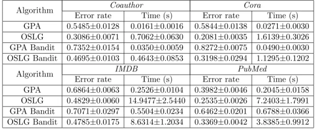
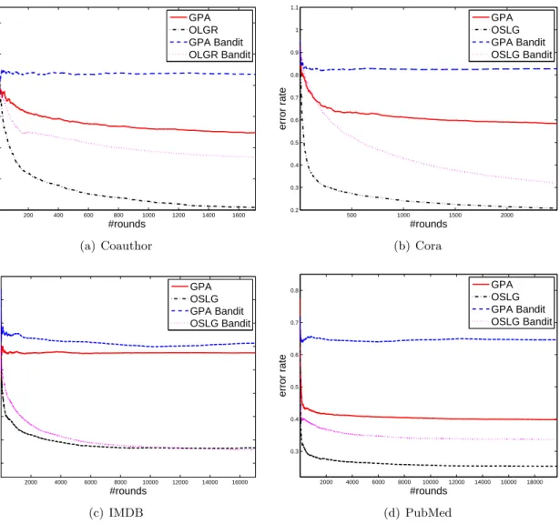
The proposed online learning algorithms in Chapter 3 on a graph are limited to binary classification. Moreover, they require accessing the full label information, where the label oracle needs to return the true class label after the learner makes classification of each node. Evidently, providing partial feedback sometimes is more efficient and reliable than providing the label. Note that in conventional online learning, a true label is revealed and therefore it requires much higher labeling cost. In many applications, it is more realistic to provide partial feedback rather than full information. For example, the label oracle will return a single bit indicating whether the prediction is correct or not, instead of the true class label. This is also known as bandit feedback. I present an online multi-class classification algorithm with bandit feedback, namely Online Spectral Learning on a

(16)

Graph with Bandit Feedback (OSLG Bandit). I use upper-conﬁdence bound technique to trade oﬀ the exploration and exploitation of label information. We show that its regret bound is only a√T

factor worse than OSLG in the full information setting. Note that online learning in a network with partial feedback has wide applications for recommendation system and advertisement placement in a network. As far as we know, this is the ﬁrst algorithm of online learning with bandit feedback on a graph. I will describe it in details in Chapter 4.

1.5

Notation

Given a weighted graph G= (V, E), where each nodevi ∈V corresponds to a data point xi, and

the weightSij of edge eij ∈E reﬂects the aﬃnity betweeni-th node and the j-th node. S∈Rn×n

is called adjacency matrix of the graph. For undirected graphs,S is symmetric, while for directed graphs,Sis asymmetric. In the setting of classiﬁcation, some of the nodes on the graph are labeled, i.e.,yi ∈ {±1}, while the remainder are unlabeled, i.e.,yi = 0. And our goal is to predict the labels

of those unlabeled nodes.

Throughout this thesis, we will use lower case letters to denote scalars, lower case bold letters to denote vectors (e.g.,w), upper case letters to denote the elements of a matrix or a set, and bold-face upper case letters to denote matrices (e.g., A). 0 is a vector of all zeros with appropriate length, and 1 is a vector of all ones with appropriate length. I is an identity matrix with an appropriate size. We use w⊤ denote the transpose of a vectorw, and A−1 the inverse of a matrixA. Given a matrixL,L†denotes its pseudo inverse. diag(σ1, . . . , σn) denotes a diagonal matrix with diagonal

elements equal to σi’s. Furthermore, ∥ · ∥ denotes the ℓ2-norm of a vector, ∥ · ∥F denotes the

Frobenius norm of a matrix, and∥x∥A denotes the matrix-induced norm∥x∥A=

√ x⊤Ax.

1.6

Organization of the Thesis

The rest of this thesis is organized as follows.

In Chapter 2, I present an active learning algorithm in a network based on generalization error bound minimization.

(17)

classiﬁca-tion, namely Learning with Local and Global Consistency method (OLLGC). Based on OLLGC, I present a selective sampling algorithm, namely Selective Sampling with Local and Global Consis-tency (SSLGC). The regret bounds of both algorithms are analyzed.

In Chapter 4, I first extend the online binary classification algorithm proposed in Chapter 3 to online multi-class classification, from the perspective of spectral learning. Then I study online learning on a graph with bandit feedback. I propose an algorithm based on online spectral learning. The regret bounds of both algorithms are derived.

(18)

Chapter 2

Active Learning in a Network

2.1

Introduction

In many practical machine learning problems, the acquisition of labeled data is often expensive and/or time consuming. This motivates Active Learning [17], which attempts to select the most informative data points for labeling to reduce the labeling cost. Traditional active learning meth-ods [61] [63] [38] focus on the data which are represented by vectors. However, in many real-life applications, the data are represented by a graph, e.g., bibliographic networks. Moreover, the data which are represented by vectors can be transformed into a graph by standard techniques widely used in graph-based semi-supervised learning [69] [67]. Therefore, active learning on a graph is an alternative of practical interest to traditional active learning and has received increasing attention. Depending on whether there is an interaction between the learner and the oracle, active learning can be roughly categorized into two families. One isadaptive active learning, such as SVM active learning [61], and agnostic active learning [3], which is able to use previous labels to determine the next point to label. The other family isnonadaptiveactive learning, which is appealing because it is able to select a batch of data points without training a classiﬁer. For example, optimal experimental design methods [63] [38] have been used for nonadaptive active learning. In our study, we mainly focus on nonadaptive active learning.

In recent years, many active learning methods on a graph have been proposed, motivated by diﬀerent criteria of “informative” data. For example, [37] derived a deterministic error bound for Minimum Cut-based semi-supervised learning approach [7], which shows that the prediction error is small if the graph cut size is large. This suggests a label selection method to choose the labeled nodes to maximize the graph cut size. Therefore, they proposed a heuristic algorithm to maximize the graph cut for active learning. [36] generalized the error bound in [37] by replacing

(19)

the graph cut with an arbitrary symmetric submodular function, and also proposed an improved algorithm to maximize the graph cut using submodular function maximization technique. [37] proposed a probabilistic error bound that motivates an active learning method, which ﬁrst clusters the graph and then randomly chooses a node in each cluster. [44] proposed to select the most informative nodes by minimizing the prediction variance ofGaussian Filed and Harmonic Function

(GFHF) [69]. All the active learning methods mentioned above are non-adaptive. Another line of research [12] [6] has considered adaptive active learning, where the labels for the nodes of a graph are queried and predicted in an iterative way.

In this chapter, we aim to develop a non-adaptive active learning method on a graph, which theoretically guarantees a good generalization performance. To achieve this goal, it is natural to consider the generalization error of a specific classifier on a graph. In particular, we chooseLearning with Local and Global Consistency(LLGC) [67] as the classifier on a graph, because it is comparable to or even better thanMinimum Cut (MinCut) [7] and GFHF [69]. We present a data-dependent generalization error bound for LLGC using the tool of transductive Rademacher Complexity [20], which is an extension of inductive Rademacher Complexity [4] and measures the richness of a class of real-valued functions with respect to a probability distribution. We show that the empirical transductive Rademacher complexity is a good surrogate for active learning on a graph. Thus we propose to actively select the nodes by minimizing the empirical transductive Rademacher com-plexity of LLGC on a graph. The resulting active learning method is a combinatorial optimization problem. In order to optimize it effectively, we present a sequential optimization algorithm. It is worth noting that our proposed active learning method tends to result in small generalization error for LLGCa. Experiments on benchmark datasets show that the proposed method outperforms the state-of-the-art active learning methods on a graph.

The remainder of this chapter is organized as follows. In Section 2.2, we present a generalization error bound for LLGC. In Section 2.3, we present a criterion for active learning and its optimization algorithm. The experiments are demonstrated in Section 2.5. Finally, we draw conclusions in Section 2.6.

a

(20)

2.2

Analysis of Learning with Local and Global Consistency

2.2.1 Review of LLGC

There exist bunches of graph-based (semi-supervised) learning methods, e.g., Minimum Cut (Min-Cut) [7], Gaussian Field and Harmonic Function (GFHF) [69] and Learning with Local and Global Consistency (LLGC) [67]. In this work, we focus on LLGC because it is the state-of-the-art method and amenable to theoretical analysis.

In order to preserve the topological properties of a graph, LLGC [67] assumes that if two nodes xi andxj are connected in the graph, then the labels of these two nodes tend to be similar to each

other. The is also known as homophily assumption in a network. Given a symmetric adjacency matrix W ∈Rn×n of the graph, and let f(xi) be the label of node xi produced by a classiﬁer f,

the above assumption can be mathematically formulated as: 1 2 n ∑ i,j=1 (fi−fj)2Wij =f⊤Lf, (2.1)

where fi is a shorthand for f(xi), f = [f1, . . . , fn]⊤,D is a diagonal matrix, called degree matrix,

withDii=

∑n

j=1Wij,L=D−W is the combinatorial graph Laplacian [16], and Iis an identity matrix of appropriate size. (2.1) is calledGraph Regularization. Intuitively, the objective function incurs a heavy penalty if neighboring points xi and xj are mapped far apart.

In the setting of binary classiﬁcation, LLGC pursues a function f by minimizing the following criterion min f 1 2∥f −y∥ 2 2+ µ 2f ⊤_Lf_,

where µ >0 is a regularization parameter, which controls the balance between the loss and label smoothness. y is the label vector with y= [y1, y2, . . . , yn]⊤.

2.2.2 Generalization Error Bound for LLGC

In this subsection, we derive a generalization error bound for LLGC using the tool of transductive Rademacher complexity for general function classes [20].

(21)

Definition 2.1. [20] For a ﬁxed sample set S ={x1, . . . ,xn} generated by a distributionDX on a

set X and a real-valued function class F with domain X, the empirical transductive Rademacher complexity of F is the random variable

ˆ Rl+u(F) = ( 1 l + 1 u ) Eσ [ sup f∈F l+u ∑ i=1 σif(xi) ] ,

where l+u=n, and σ= (σ1, . . . , σn)T are independent random variables such that

σi =            1 w.p. p −1 w.p. p 0 w.p. 1−2p, where 0≤p≤ 1₂. The transductive Rademacher complexity is

Rl+u(F) =Ex [ ˆ Rl+u(F) ] .

Note that for the case p = 1₂ and l = u, the transductive Rademacher complexity coincides with the standard inductive deﬁnition [4] up to a normalization factor 1_l +_u1. We set p= _nlu2 in the

following derivation.

Intuitively speaking, transductive Rademacher complexity measures the richness of a class of real-valued functions with respect to a probability distribution.

Theorem 2.1. [20] Fixδ ∈(0,1), and let F be a class of functions mapping from X × Y to[0,1]. Let c0 = √ 32 ln(4e) 3 and Q = 1 l + 1

u. For any ﬁxed sample set {(xi, yi)} n

i=1, with probability 1−δ

over random draws of a subsample of size l, every f ∈ F satisﬁes

err(f)≤errˆ (f) + ˆRl+u(F) +c0Q

√

min(l, u) +√2Qln(1/δ),

where err(f) is the expected error on the unlabeled data, and errˆ (f) is the empirical error on the labeled data.

The above error bound is quite general and applicable to various transductive learning algo-rithms if an empirical transductive Rademacher complexity ˆRl+u(F) of the function classF can be

(22)

found eﬃciently. It also implies that in order to prove the generalization error bound for LLGC, it is suﬃcient to give an estimation of the empirical transductive Rademacher complexity for the following function class.

Definition 2.2. The function class of LLGC isFl={f = (µL+I)−1y,||y||2 ≤ √

l}.

Note that there are llabeled data with yi∈ {±1}, therefore,||y||2≤ √

l.

In the following, we present two theorems, which serve as the theoretical foundation of our proposed method in this chapter.

Theorem 2.2. The empirical transductive Rademacher complexity of the function classFlis upper

bounded as ˆ Rl+u(Fl)≤ √ 2 utr((µL+I)− 2₎_,

where I is an identity matrix.

Proof. The empirical Rademacher complexity of the function class Fl is computed as

ˆ Rl+u(Fl) = ( 1 l + 1 u ) Eσ [ sup f:||y||2≤ √ l y⊤(µL+I)−1σ ] ≤ ( 1 l + 1 u ) Eσ [ sup f:||y||2≤ √ l ||y||2||(µL+I)−1σ||2 ] ≤ ( 1 l + 1 u )_√ lEσ   v u u t∑n i,j=1 σiσj((µL+I)−2)ij   ≤ ( 1 l + 1 u )_√ l √ 2lu n2tr ((µL+I)−2) = √ 2 utr ((µL+I)− 2₎_,

where the ﬁrst inequality holds due to the Cauchy-Schwarz’s inequality and the third inequality holds due to the Jensen’s inequality.

Using Theorem 2.1 and Theorem 2.2, we obtain the following generalization error bound for LLGC.

(23)

Theorem 2.3. Fix δ ∈(0,1), and letF be a class of functions mapping from X × Y to[0,1]. Let c0 = √ 32 ln(4e) 3 and Q= 1 l + 1

u. For any ﬁxed sample set {(xi, yi)} n

i=1, with probability 1−δ over

random draws of a subsample of size l, every f ∈ F satisﬁes

err(f)≤errˆ (f) + √ 2 utr((µL+I)− 2_{) +}_c 0Q √ min(l, u) +√2Qln(1/δ).

2.3

Active Learning via Error Bound Minimization

The generic problem of non-adaptive active learning on a graph is as follows. Given a weighted graph G = (V, E), V is the pool of candidate nodes, our goal is to ﬁnd a subset L ⊂ V, which contains the most informative l nodes, namely active set or labeled set. Let U = V \ L be the unlabeled set. Given a graph Laplacian matrix L associated with the graph, LLL denotes

the principal submatrix corresponding to the labeled setL, LU U denotes the principal submatrix

corresponding to the unlabeled setU, andLLU denotes the submatrix which interrelates the labeled

set Lwith unlabeled set U.

2.3.1 Objective Function

From Theorem 2.3, we can see that the expected error on the unlabeled data is upper bounded by the empirical error on the labeled data plus the empirical transductive Rademacher complexity

ˆ

Rl+u(Fl) and the conﬁdence termc0Q

√

min(l, u)+√2Qln(1/δ). It is easy to check that, the larger the number of labeled samples (l) is, the tighter the bound will be. In other words, the expected error on the unlabeled data will be approximated by the empirical error more accurately. Ideally we should minimize the expected error on the unlabeled data by jointly minimizing the empirical error on the labeled data and ˆRl+u(Fl). However, in the setting of non-adaptive active learning

on a graph, we do not know the label of a given node until we select this node. That means we cannot estimate ˆerr(f) before we label the nodes and train a classiﬁer. Hence the only term we can control is the empirical transductive Rademacher complexity. In other words, minimizing ˆRl+u(Fl)

is a surrogate to guarantee small expected error. Therefore, we present an active learning criterion by minimizing the upper bound of empirical transductive Rademacher complexity for LLGC as

(24)

follows, arg min L⊂V tr ( (µLLL+I)−2 ) , (2.2)

where we ignore the constant scalers and square root symbol. Note that LLL is computed based

on the selected l samples, i.e.,L.

The above optimization problem is a combinatorial optimization problem. Finding the global optimal solution is NP-hard. Motivated by the success of sequential minimization algorithm in some existing experimental design approaches [63] [38] [44], we present a simple yet eﬀective sequential optimization algorithm as follows.

2.3.2 Sequential Optimization

We introduce a selection matrixS∈Rn×l, which is deﬁned as

Sij =     

1, ifxi is selected as the j-th point inL

0, otherwise.

It is easy to check that each column of Shas one and only one 1, each row has at most one 1, and STS=I. The constraint set forS can be deﬁned as

S ={S|S∈ {0,1}n×l,S⊤1=1,S1≤1} ={S|S∈ {0,1}n×l,S⊤S=I}.

Then LLL can be represented byS⊤LS. Therefore, (2.2) can be equivalently written as

arg min S⊂Str ( (µS⊤LS+I)−2 ) . (2.3)

(25)

Λ= diag(λ1, . . . , λn) is a diagonal matrix whose diagonal elements are eigenvalues. We have tr ( (µS⊤LS+I)−2 ) = tr ( (µS⊤UΛU⊤S+I)−2 ) = tr ( (S⊤U(µΛ+I)U⊤S)−2 ) = tr ( (S⊤UΣU⊤S)−1 ) = tr ( (S⊤UΓU⊤S+I)−1 ) , where Σ = diag((µλ1+ 1)2, . . . ,(µλn+ 1)2 ) , Γ = diag((µλ1+ 1)2−1, . . . ,(µλn+ 1)2−1 ) , and we use the fact thatS⊤UU⊤S=I.

Using the Woodbury matrix identity [23], we have

(S⊤UΓU⊤S+I)−1 =I−S⊤U(Γ−1+U⊤SS⊤U)−1U⊤S. Hence tr ( (S⊤UΓU⊤S+I)−1 ) =l−tr ( S⊤U(Γ−1+U⊤SS⊤U)−1U⊤S ) =l−tr((Γ−1+UTSS⊤U)−1(Γ−1+U⊤SS⊤U−Γ−1)) =l−n+ tr ( (Γ−1+U⊤SS⊤U)−1Γ−1 ) ,

where Γ−1 is a diagonal matrix whose i-th diagonal element is ₍_µλ 1

i+1)2−1

b_{. Therefore, the} opti-mization problem in (2.3) is equivalent to

arg min L⊂Vtr ( (Γ−1+U⊤_LUL)−1Γ−1 ) ,

where UL = S⊤U is a submatrix of U. More specially, UL consists of the rows in U which

corresponds to the selected nodes.

Let H0 = Γ−1. Suppose k nodes have been selected, denoted by Lk, which correspond to

b

Since the smallest eigenvalue of graph Laplacian is 0,Γ−1 is ill-deﬁned. In our implementation, we resolve this problem by replacing the zero eigenvalue with a suﬃcient small value, e.g., 1e−6.

(26)

ULk ∈ R

k×n_{. Let} _H

k =Γ−1+U⊤LkULk, then the (k+ 1)-th node can be selected by solving the

following optimization problem

ik+1 = arg min i⊂V /Lk tr ( (Hk+uiu⊤i )−1Γ−1 ) , (2.4)

whereui is the transpose of the i-th row ofU (thus a column vector).

By using the Sherman-Morrison formula [23], we have

(Hk+uiu⊤i )−1 =H−k1− H−_k1uiu⊤i H−k1 1 +u⊤_i H−_k1ui . Therefore, tr ( (Hk+uiu⊤i )−1Γ−1 ) = tr(H−_k1Γ−1)−u ⊤ i H−k1Γ− 1_H−1 k ui 1 +u⊤_i H−_k1ui .

Since tr(H−_k1Γ−1) is a constant given H−_k1, the optimization problem in (2.4) is equivalent to

ik+1 = arg max

i⊂V/Lk

u⊤_i H−_k1Γ−1H−_k1ui

1 +u⊤_i H−_k1ui

. (2.5)

Once the (k+1)-th node is selected,H−_k₊₁1 can be updated based onH−_k1, by using the Sherman-Morrison formula again,

H−_k₊₁1 =H−_k1−H −1 k uik+1u⊤ik+1H −1 k 1 +u⊤_i k+1H −1 k uik+1 . (2.6)

Note that H−_k₊₁1 is updated by matrix (vector) multiplication and addition, rather than matrix inverse. Therefore, this process is eﬃcient.

In summary, we present the whole algorithm for active learning on a graph in Algorithm 2.1.

2.3.3 Complexity Analysis

The computational complexity of Algorithm 2.1 includes two parts. The ﬁrst part is eigen-decomposition of the adjacency matrix W. For a graph whose average node degree is k, the Lanczos algorithm [23] can be used to eﬃciently compute the eigenvectors of the eigen-problem

(27)

Algorithm 2.1 Active Learning on a Graph via Generalization Error Bound Minimization (Bound)

Input: Adjacency matrixW, number of nodes to select l, regularization parameterµ; Compute L=I−D−12WD−

1 2

Perform eigen decomposition L=UΛU⊤ Initialize H0=Γ−1,L0 =∅

for k= 0→l−1 do

Compute ik+1 = arg maxi⊂V\Lk

u⊤_iH−1_k Λ−1H−1_k ui 1+u⊤_iH−_k1ui ; UpdateLk+1 =Lk∪ {ik+1} UpdateH−_k₊₁1 =H−_k1−H −1 k uik+1u⊤ik+1H −1 k 1+u⊤_ik +1H −1 k uik+1 end for

within O(tn2k), where t is the number of iterations in Lanczos. The second part is the sequential optimization algorithm, whose complexity is O(n2l) where l is the number of selected nodes, i.e., |L|. Hence the total time complexity isO(n2₍_tk₊_l_{)), which is applicable to medium-scale graphs.}

2.4

Analysis of Homophily Assumption

The major assumption behind LLGC for networked data is the homophily assumption, which is mathematically formulated by (2.1). In this section, we aim at analyzing the homophily assumption, to show when will it holds. To the best of our knowledge, this is the ﬁrst theoretical analysis of homophily assumption.

It is unclear how to analyze homophily assumption without making any assumption on the joint distribution of a graph. Therefore, we restrict our analysis into the context of planted partition model [53], which is a popular random graph model for graph clustering (and classiﬁcation). It is also known as stochastic block model.

We ﬁrst brieﬂy review planted partition model. Planted partition model is a generative model for random graphs. A un-weighted graph G = (V, E) generated from this model has a hidden partition V1, . . . , Vc such that V1∪V2∪. . .∪Vc =V, andVi∩Vj =∅ fori̸=j. If a pair nodes u

and v both lie in someVi, then P((u, v) ∈E) =p; Otherwise, P((u, v)∈E) =q. Here p, q∈[0,1]

are parameters of the model, and we assume p > q. Hence, it is more likely to to have an edge between nodes within the same cluster than it is between nodes from diﬀerent clusters. We will show that the quantity p−q is crucial for homophily assumption.

(28)

Since W is an observation of the underlying planted partition model, we introduce the expec-tation of the random adjacency matrix W, denoted by ¯W. We have

¯ Wij =            0 ifi=j p ifyi =yj and i̸=j q ifyi ̸=yj (2.7)

In the special case that c = 2, without loss of generality, we assume that the ﬁrst n/2 nodes belong to one class, and the rest nodes belong to the other class for simplicity. Then according to [53], the eigenvalues ¯λ1≥. . .≥¯λn of ¯W are

n(p+q) 2 −p, n(p−q) 2 −p, |{z}−p n−2 ,

and the eigenvector of ¯W corresponding to ¯λ1= 0 and ¯λ2 =nq are

v1=1n, v2 = 1 √ n    1n/2 −1_n/₂   .

Let ¯L be the corresponding graph Laplacians of ¯W, it is easy to show that the eigenvalues ¯ σ1 ≤σ¯2≤. . .≤σ¯n of ¯L are 0, nq, n 2(p−q) +nq, . . . , n 2(p−q) +nq | {z } n−2 ,

and the corresponding eigenvectors are identical to the eigenvectors of ¯W.

Thus, the expectation of the smoothness term in (2.1) can be expressed as follows

E  1 2 n ∑ i,j=1 (fi−fj)2Wij   = 1 2 n ∑ i,j=1 (fi−fj)2W¯ij =f⊤Lf¯ .

(29)

Intuitively speaking, in order to make the optimal solution of binary LLGC (as in (2.2)) to be the same as v1 up to some constant scaling (which results in perfect classification with zero classification error), we need the eigen gap between ¯σ2 and ¯σ3 to be sufficiently large. In other words, we require ¯σ3−σ¯2 =n/2(p−q) to be sufficiently large. Roughly speaking, in order to make ¯

σ3−σ¯2 be O(1),p−q should beO(1/n). Of course, ifp−q= Ω(1/n), that would be better. In the case that c >2, for the sake of analysis, without loss of generality, we assume that each cluster has the same size, and the matrix ¯W has a block diagonal structure, i.e., the elements in thei-th class have indices from n_c(i−1) + 1 to n_ciin{1, . . . , n}. According to [22], the eigenvalues ¯ λ1≥λ¯2 ≥. . .≥λ¯n of ¯W are (n c −1 ) p+ (n−n c)q, n c(p−q)−p, . . . , n c(p−q)−p | {z } c−1 , −_| p, . . . ,_{z −p_} n−c .

and the eigenvectors corresponding to the largest ceigenvalues of ¯Lare

v1=1n, vjk =      √_c n ifj∈ { n c(k−1) + 1, . . . , n ck} 0 otherwise , j = 1, . . . , d, k= 2, . . . , c

Again, it is easy to show that the eigenvalues ¯σ1≤¯σ2 ≤. . .≤σ¯n of ¯Lare

0, nq, . . . , nq_{| {z }} c−1 , n c(p−q) +nq, . . . , n c(p−q) +nq | {z } n−c . (2.8)

and the corresponding eigenvectors are the same as the eigenvectors of ¯W.

Thus, the expectation of the smoothness term for c >2 can be expressed as follows

E  1 2 c ∑ k=1 n ∑ i,j=1 (fik−fjk)2Wij   = 1 2 n ∑ i,j=1 (fik−fjk)2W¯ij = c ∑ k=1 f_k⊤Lf¯ k.

(30)

where fk, k = 1, . . . , c are the c classiﬁers for each class, and fk, k = 1, . . . , c are the prediction

scores of the nodes for each class. For more details, please refer to Chapter 3.

Analogously, in order to make the optimal solutions of multi-class LLGC to be the same as v1, . . . ,vc up to some constant scalings (which result in perfect classiﬁcation with zero classiﬁcation

error), we need the eigen gap between ¯σc and ¯σc+1to be suﬃciently large. In other words, we require ¯

σc+1−σ¯c =n/c(p−q) to be suﬃciently large. In order to make ¯σc+1−¯σc beO(1),p−q should be

O(c/n), where c is the number of classes. Therefore, the larger the number of classes, the bigger

p−q should be to achieve good classiﬁcation. It is better to havep−q = Ω(c/n)

Note that the above argument is in the light of expectation. In order to deliver similar results in the light of high probability, we need more involved argument, which will be explored in the future. Moreover, the above analysis is restricted to the simpliﬁed case that each class has the same size. In the case that each class has a diﬀerent size, the result will become more complicated. We will analyze it in the future as well.

2.5

Experiments

In this section, we evaluate the proposed method on real-world datasets, and compare it with the state-of-the-art active learning methods on a graph. Recall that the input of active learning methods on a graph is an adjacency matrix.

2.5.1 Datasets

In our experiments, we use three real-world benchmark datasets to evaluate the active learning methods.

Cora contains the abstracts and references of about 34,000 research papers from the computer science community. The task is to classify each paper into one of the subﬁelds of data structure (DS), hardware and architecture (HA), machine learning (ML), and programming language (PL), based on the citation relation between the papers. We only use the link information of this dataset. We choose DS and PL subsets to form two datasets. For each dataset, the largest connected component of the graph is used. Since the adjacency matrix of the Cora dataset is directed, we symmetrize it by max(W,W⊤).

(31)

Coauthor is an undirected co-author graph data extracted from the DBLPc database in four areas: machine learning, data mining, information retrieval and database. It contains a total of 1711 authors, each of which is represented by a node. The edge between each pair of authors is weighted by the number of papers they co-authored. Each class contains about 400 authors. This graph is already connected.

In order to show that the homophiply assumption holds in these datasets, we will estimate a planted partition model on each dataset. More speciﬁcally, we will estimate p and q for each dataset, using the adjacency matrix of the graph, as well as the groundtruth labels. We summarized the estimated p,q and p−q in Table 2.1. In addition, we also show the value of c/n.

Table 2.1: Justiﬁcation of the homophily assumption on the three datasets Dataset Cora (DS) Cora (PL) Coauthor

p 0.0223 0.0110 0.0288

q 0.0011 0.0007 0.0011

p−q 0.0212 0.0103 0.0277

c/n 0.0178 0.0061 0.0023

We can see that on these three datasets, the value of p−q is at least in the same order ofc/n. According to the analysis in Section 2.4, it indicates that the homophily assumption on these three datasets should be valid. Thus, we can hope that LLGC performs well on these three datasets.

2.5.2 Methods & Parameter Settings

To demonstrate the eﬀectiveness of our proposed method, we compare the following active learning approaches.

• Random Sampling (Random) uniformly selects nodes from the candidate set. It is the simplest baseline for active learning.

• Variance Minimization (VM) [44] is a recently proposed method, which is motivated by GFHF and minimizing the prediction variance.

(32)

• METIS[37]: it uses the METIS clustering method [49] to divide a graph intolclusters, and randomly chooses one data point from each cluster.

• Ψ Maximization (Ψ-Max) [36]: it is solved by submodular function maximization, which performs better than the heuristic optimization algorithm proposed in [37].

• Generalization Error Bound Minimization (Bound) is our proposed method. It is motivated by Theorem 2.3. There is one parameterµtunable. Throughout our experiments, we simply ﬁxµ= 0.01.

After selecting the nodes by active learning, we train a classifier on the graph to do classification. In our experiments, we tried three classifiers: LLGC, GFHF and MinCut. The reason why we tried these three classifiers is obvious, because the proposed active learning method is built upon LLGC, VM is motivated by GFHF and Ψ-Max is designed for MinCut. There is a parameter for LLGC, i.e., µ, which is tuned by 3-fold cross validation on the selected labeled set over the grid {0.01,0.1,1,10,100}.

2.5.3 Experimental Setup

In order to randomize the experiments, in each run of experiments, we restrict the pool of the candidate nodes to be selected from a random sampling of 50% of the total nodes. The random split was repeated 10 times. For each dataset, we let the active learning methods incrementally choose {10,20, . . . ,160}nodes from the training set to label. We evaluate different active learning methods combined with different classifiers. We compute the mean classification accuracy on all the unlabeled nodes, that is, the unselected nodes in the pool plus the remaining 50% nodes.

2.5.4 Classification Results

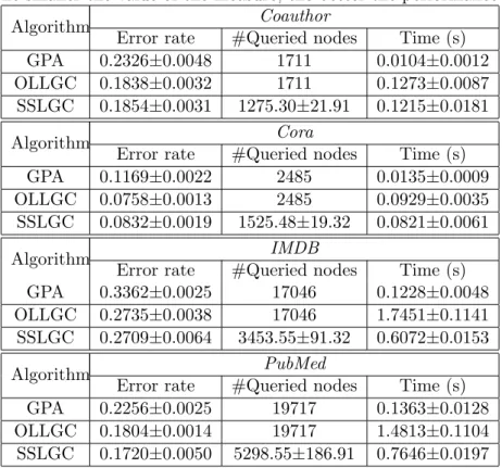
The experimental results evaluated on the unlabeled data are shown in Figures 2.1 and 2.2. In all subfigures, the horizontal axis represents the number of labeled nodes, while the vertical axis is the averaged classification accuracy over 10 runs. The experimental result of MinCut is much worse than LLGC and GFHF for all the active learning methods, because it usually results in a very unbalanced classification. Therefore, we omit its result.

(33)

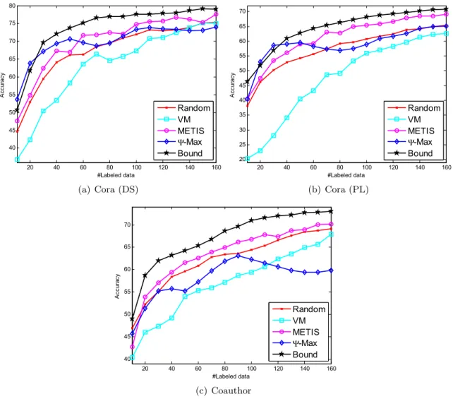
20 40 60 80 100 120 140 160 40 45 50 55 60 65 70 75 80 #Labeled data A c c u ra c y Random VM METIS Ψ-Max Bound (a) Cora (DS) 20 40 60 80 100 120 140 160 20 25 30 35 40 45 50 55 60 65 70 #Labeled data A c c u ra c y Random VM METIS Ψ-Max Bound (b) Cora (PL) 20 40 60 80 100 120 140 160 40 45 50 55 60 65 70 #Labeled data A c c u ra c y Random VM METIS Ψ-Max Bound (c) Coauthor

Figure 2.1: Comparison of active learning methods on (a) Cora (DS); (b) Cora (PL); and (c) Coauthor using LLGC evaluated on all the unlabeled data.

From Figures 2.1 and 2.2, we observe that the proposed method (Bound) consistently outper-forms other methods in most cases using either LLGC or GFHF. It is appealing because even though our method is built upon the error bound minimization of LLGC, it is also much better than other methods using GFHF. But note that our method using LLGC achieves marginally bet-ter performance than using GFHF. On the Cora datasets, when the number of labeled nodes is small, e.g., less than 30, our method and Ψ-Max usually perform the best. On the other cases, our method is much better than the second best method. The superior performance of our method is attributed to its theoretical foundation, which guarantees that the classiﬁer can achieve small generalization error on the unlabeled data.

(34)

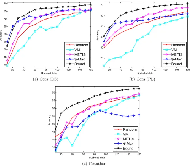
20 40 60 80 100 120 140 160 40 45 50 55 60 65 70 75 80 #Labeled data A c c u ra c y Random VM METIS Ψ-Max Bound (a) Cora (DS) 20 40 60 80 100 120 140 160 20 30 40 50 60 70 #Labeled data A c c u ra c y Random VM METIS Ψ-Max Bound (b) Cora (PL) 20 40 60 80 100 120 140 160 35 40 45 50 55 60 65 70 #Labeled data A c c u ra c y Random VM METIS Ψ-Max Bound (c) Coauthor

Figure 2.2: Comparison of active learning methods on (a) Cora (DS); (b) Cora (PL); and (c) Coauthor using GFHF evaluated on all the unlabeled data.

VM is usually worse than random sampling. The reason is that minimizing the prediction variance does not guarantee the quality of predictions on the unlabeled data.

The performance of METIS is usually comparable to or even better than that of Ψ-Max. Al-though METIS has a solid theoretical foundation, the corresponding criterion is so diﬃcult that we have to solve it by a clustering algorithm [49] followed by a heuristic sampling, which sacriﬁces its performance.

In summary, our method together with LLGC is the most promising combination, which is consistent with our theory.

(35)

2.6

Conclusions

The main contributions of this chapter are: (1) We present a transductive error bound for LLGC; (2) we present an active learning criterion for graph data via minimizing the empirical transductive Rademacher complexity of LLGC; and (3) we present a simple algorithm to optimize the active learning criterion. In the future, we plan to develop a more scalable algorithm to solve (2.2).

(36)

Chapter 3

Selective Sampling in a Network

In previous chapter, I have introduced active learning in a network (i.e., on a graph). I will introduce online learning in a network in this chapter, and combine the idea of active learning and online learning together to study selective sampling in a network.

3.1

Introduction

Selective sampling [21] [13] is an active variant of online learning [14] in which the learner is allowed to adaptively query the labels of a sequence of examples. The learner’s goal is to achieve a good trade-oﬀ between error rate and the number of queried labels. This can be viewed as an abstract protocol for interactive learning applications. Recently, several advanced selective sampling algorithms [11] [54] were proposed, demonstrating more promising results than traditional passive online learning. However, we note that existing selective sampling algorithms are speciﬁcally designed for vector-based data.

Graphs have recently received significant attention because of their increasingly important role in real life applications. Examples include the friendship network in Facebooka_{, co-author and} citation networks inDBLPb, and the World Wide Web. In these applications, the data (nodes) are not independent and identically distributed (i.i.d.) as is typically assumed in statistical learning applications, because of the impact of the linkage structure of the graph. Learning a function defined on a graph from a set of labeled nodes has been studied extensively in machine learning both in off-line and online settings. More specifically, in the offline learning scenario, a majority of the literature is often referred to as graph-based semi-supervised learning [69] [67]. On the other hand, the pioneering work towards online learning on a graph is probably [42]. Inspired by this

a_{http://www.facebook.com} b

(37)

work, the state-of-the-art Graph Perceptron Algorithm (GPA) was proposed in [41] and further analyzed in [40] [39].

Based on the above observation, a natural question arises as to whether we can design selective sampling algorithms for graphs. The results of this chapter show that the answer is in the affir-mative. In this chapter, we propose to study selective sampling on a graph. Our work is built on a well-known model on a graph, namely learning with local and global consistency. This model is a state-of-the-art model on a graph and is particularly amenable to analysis in the context of selective sampling. We first present an online version of the well-known Learning with Local and Global Consistency method (OLLGC). It is essentially a second-order online learning algorithm, and can be seen as an online ridge regression in the Hilbert space of functions defined on a graph. We prove its regret bound in terms of cut size of a graph. Based on OLLGC, we present a selec-tive sampling algorithm, namely Selecselec-tive Sampling with Local and Global Consistency (SSLGC), which queries the labels of nodes based on the confidence of the linear function on a graph. We also derive a bound on the label complexity of our proposed algorithm. Lastly, in order to scale the proposed algorithms as well as existing online learning algorithms to large graphs, we dis-cuss the low-rank approximation technique for graph kernels. Experiments on benchmark graph datasets show that OLLGC outperforms GPA [41] substantially. Furthermore, the selective sam-pling algorithm (SSLGC) achieves comparable or even better results than OLLGC, while querying substantially fewer nodes. Moreover, SSLGC provides superior results to random sampling.

The main contributions of this chapter are three-fold: (1) we present an online learning with local and global consistency (OLLGC), and prove its regret bound; (2) we present a selective sampling algorithm on a graph based on OLLGC, and derive its bound on label complexity; and (3) we analyze the low-rank approximation of graph kernels, which enables greater scalability of our algorithms as well as existing algorithms, when the graphs are large.

The remainder of this chapter is organized as follows. In Section 3.2, we brieﬂy review the related literature. In Section 3.3, we present an online version of learning with local and global consistency, followed by its regret bound. In Section 3.4, we devise a selective sampling algorithm on a graph based on the online algorithm derived in previous section, and analyze its bound on the label complexity. We discuss and analyze the low-rank approximation of graph kernels for

(38)

online algorithms in Section 3.5. The experiments on benchmark graph datasets are demonstrated in Section 3.6. We present the conclusions in Section 3.7. The detailed proofs are included in Section 3.8

3.2

Related Work

For ease in exposition, we brieﬂy discuss online learning, active learning and selective sampling, in the context of both vector-based data and graph data.

3.2.1 Online Learning

Online learning has been studied extensively in the machine learning community. In the past several decades, a variety of online learning algorithms have been proposed. Due to the sequential nature of online learning, it is very suitable to be applied to big data from many real-world applications. Roughly speaking, online learning algorithms can be categorized into ﬁrst-order algorithms [56] [50] and second-order algorithms [10] [19]. In general, second-order online algorithms are better than ﬁrst-order online algorithms [43].

The extension of online learning to graph data was originally studied in [42]. After that work, the well-known Graph Perceptron Algorithm (GPA) was proposed in [41] and further analyzed in [40] [39]. It is worth noting that the setting of online learning on a graph is essentially transduc-tive, where the whole graph is already provided, but the learner is presented with the nodes in a sequential manner. This is different from theinductive paradigm for vector-based online learning. In addition, all the online learning algorithms on a graph mentioned before are first-order algo-rithms. Note that the first contribution of our paper, i.e., online learning with local and global consistency is a second-order algorithm on a graph, which is better than first-order algorithms.

3.2.2 Active Learning

Active learning [17] [61] aims to minimize the required level of acquisition of labeled data by actively selecting a few carefully chosen examples to query the oracle for their labels. There are several papers on active learning on a graph. For instance, [5] proposed an eﬀective label acquisition for collective classiﬁcation. [6] proposed an active learning algorithm for networked data based on

(39)

ensemble and relational learning. Yet, there is no theoretical guarantee that these methods are better than random sampling. [12] studied active learning on a graph and trees. [44] proposed a nonadaptive active learning method by minimizing the variance of Gaussian Field and Harmonic Function (GFHF) [69]. In our previous work [35], we proposed a nonadaptive active learning approach on a graph, by minimizing the data-dependent error bound of LLGC [67], which was shown to be better than [44].

3.2.3 Selective Sampling

Selective sampling [13] [11] combines the idea of online learning and active learning. Similar to online learning, a selective sampling algorithm observes examples in a sequential manner. After each observation, the algorithm predicts its label. However, rather than receiving the correct label passively, the algorithm can choose whether to receive feedback indicating whether the label is correct or not. It is obvious that by using selective sampling, we need much less labeling eﬀort, since the labels of many examples can be predicted with very high conﬁdence. In other words, selective sampling is online active learning.

Linear models lend themselves well to selective sampling settings, because the variance of a classifier on an example can be viewed as a measure of confidence for the classification. If this confidence is too low, then the selective sampler will query the label and use it, along with the example, to update the linear model. For graph data, the key question is how to define anexample

as well as a linear model. We will show that learning with local and global consistency can be equivalently formulated as alinear model on a graph.

3.3

Online Learning with Local and Global Consistency

In this section, we present an online version of learning with local and global consistency (LLGC) [67]. To make our paper self-contained, we brieﬂy review LLGC.

3.3.1 Learning with Local and Global Consistency

Given a graphG= (V, E), wherevi ∈V is the i-th node of a graph, andeij ∈E is the link (edge)

(40)

the strength of the link. S∈Rn×n is called adjacency matrix of the graph. For undirected graph, S is a symmetric matrix, while for directed graph,S is asymmetric. In the setting of transductive classiﬁcation, some of the nodes in the graph are labeled, i.e., yi ∈ {±1}, while the remainder

are unlabeled, i.e., yi = 0. Our goal is to obtain a prediction about the labels of those unlabeled

nodes. Through our paper, we assume that the graph G is connected, though our results can be generalized to disconnected graphs with more involved arguments.

The basic assumption of graph regularization is based on the concept of homophily in a network. If two nodesvi and vj are linked together, then their labels are likely to be similar. Let f :V →R

be a nonparametric function deﬁned on the nodes of a graph. For an undirected graph, graph regularization [59] is mathematically written as follows:

1 2 n ∑ i,j=1 (fi−fj)2Sij =f⊤Lf, (3.1)

wherefi is the function value on thei-th node, i.e., f(vi),f = [f1, . . . , fn]⊤,Dis a diagonal matrix,

which is also referred to as the degree matrix. Theith diagonal entryDii=

∑n

j=1Sij,L=D−S

is the combinatorial graph Laplacian [16]. (3.1) is called Graph Regularization. Intuitively, the objective function incurs a heavy penalty, if neighboring nodes vi and vj are mapped far apart.

Suppose the eigen decomposition ofLisL=VΣV⊤=∑n_i₌₁σiviv⊤_i , whereΣ= diag(σ1, . . . , σn),