Florida International University
FIU Digital Commons
FIU Electronic Theses and Dissertations University Graduate School
11-7-2016
A Biologically Plausible Supervised Learning
Method for Spiking Neurons with Real-world
Applications
Lilin Guo
Florida International University, [email protected]
DOI:10.25148/etd.FIDC001243
Follow this and additional works at:https://digitalcommons.fiu.edu/etd
Part of theBioelectrical and Neuroengineering Commons,Biomedical Commons, and theSignal Processing Commons
This work is brought to you for free and open access by the University Graduate School at FIU Digital Commons. It has been accepted for inclusion in FIU Electronic Theses and Dissertations by an authorized administrator of FIU Digital Commons. For more information, please [email protected]. Recommended Citation
Guo, Lilin, "A Biologically Plausible Supervised Learning Method for Spiking Neurons with Real-world Applications" (2016).FIU Electronic Theses and Dissertations. 2982.
FLORIDA INTERNATIONAL UNIVERSITY
Miami, Florida
A BIOLOGICALLY PLAUSIBLE SUPERVISED LEARNING METHOD FOR
SPIKING NEURONS WITH REAL-WORLD APPLICATIONS
A dissertation submitted in partial fulfillment of the
requirements for the degree of
DOCTOR OF PHILOSOPHY in ELECTRICAL ENGINEERING by Lilin Guo 2016
ii To: Interim Dean Ranu Jung
College of Engineering and Computing
This dissertation, written by Lilin Guo, and entitled A Biologically Plausible Supervised Learning Method for Spiking Neurons with Real-world Applications, having been approved in respect to style and intellectual content, is referred to you for judgment.
We have read this dissertation and recommend that it be approved.
_______________________________________ Armando Barreto _______________________________________ Nezih Pala _______________________________________ Mercedes Cabrerizo _______________________________________ Wei-Chiang Lin _______________________________________ Malek Adjouadi, Major Professor
Date of Defense: November 7, 2016
The dissertation of Lilin Guo is approved.
_______________________________________ Interim Dean Ranu Jung College of Engineering and Computing
_______________________________________ Andrés G. Gil Vice President for Research and Economic Development and Dean of the University Graduate School
iii
© Copyright 2016 by Lilin Guo
iv DEDICATION
I dedicate this dissertation to my supportive husband, Tan Ma, to my lovely daughter,
Esther Ma, for making this work meaningful. I also dedicate this work to my beloved
parents. Without their patience, understanding, support, and love, the completion of this
v
ACKNOWLEDGMENTS
First and foremost, I would like to express my deepest gratitude to my advisor, Dr. Malek
Adjouadi, for his excellent guidance, caring, patience, and invaluable insights throughout
all the stages of researching and writing this dissertation, as well as for the financial support
provided to me for the completion of this dissertation. He provided unserved support during
my PhD, patiently corrected my writing and generously paved the way for my development
as a researcher. His passion and dedication are incomparable and always inspire me.
Next, I wish to express my great appreciation to my committee members, Dr. Armando
Barreto, Dr. Nezih Pala, Dr. Mercedes Cabrerizo and Dr. Wei-Chiang Lin, for their
valuable discussions improving the quality of this dissertation.
Furthermore, I would like to acknowledge the research support provided from the
Department of Electrical and Computer Engineering at Florida International University,
the support of National Science Foundation under grant Numbers: 1532061,
CNS-1642193, CNS-0959985, CNS-1042341, HRD-0833093, IIP 1338922, IIP-1230661, and
CNS-1429345, and the generous support of the Ware Foundation, which facilitated the
research essential to the completion of this dissertation.
I would also like to extent my gratitude to all the lab mates and members at the Center for
Advanced Technology and Education for creating an amazing working environment,
especially, Zhenzhong Wang, whose encouragement greatly helped me in achieving my
research goals; to the FIU community and department staffs, especially Pat Brammer and
vi
ABSTRACT OF THE DISSERTATION
A BIOLOGICALLY PLAUSIBLE SUPERVISED LEARNING METHOD FOR
SPIKING NEURONS WITH REAL-WORLD APPLICATIONS
by
Lilin Guo
Florida International University, 2016
Miami, Florida
Professor Malek Adjouadi, Major Professor
Learning is central to infusing intelligence to any biologically inspired system. This study
introduces a novel Cross-Correlated Delay Shift (CCDS) learning method for spiking
neurons with the ability to learn and reproduce arbitrary spike patterns in a supervised
fashion with applicability to spatiotemporal information encoded at the precise timing of
spikes. By integrating the cross-correlated term, axonal and synapse delays, the CCDS rule
is proven to be both biologically plausible and computationally efficient. The proposed
learning algorithm is evaluated in terms of reliability, adaptive learning performance,
generality to different neuron models, learning in the presence of noise, effects of its
learning parameters and classification performance. The results indicate that the proposed
CCDS learning rule greatly improves classification accuracy when compared to the
standards reached with the Spike Pattern Association Neuron (SPAN) learning rule and the
Tempotron learning rule.
Network structure is the crucial part for any application domain of Artificial Spiking Neural
Network (ASNN). Thus, temporal learning rules in multilayer spiking neural networks are
vii
is also developed. Correlated neurons are connected through fine-tuned weights and delays.
In contrast to the multilayer Remote Supervised Method (MutReSuMe) and multilayer
tempotron rule (MutTmptr), the newly developed MutCCDS shows better generalization
ability and faster convergence. The proposed multilayer rules provide an efficient and
biologically plausible mechanism, describing how delays and synapses in the multilayer
networks are adjusted to facilitate learning.
Interictal spikes (IS) are morphologically defined brief events observed in
electroencephalography (EEG) records from patients with epilepsy. The detection of IS
remains an essential task for 3D source localization as well as in developing algorithms for
seizure prediction and guided therapy. In this work, we present a new IS detection method
using the Wavelet Encoding Device (WED) method together with CCDS learning rule and
a specially designed Spiking Neural Network (SNN) structure. The results confirm the
ability of such SNN to achieve good performance for automatically detecting such events
viii TABLE OF CONTENTS CHAPTER PAGE 1. INTRODUCTION ... 1 1.1 Background ...1 1.2 Research Purpose ...3 1.3 Methodology ...4
1.4 Original Contribution of This Dissertation ...6
1.5 Dissertation Organization ...8
2. SPIKING NEURAL NETWORKS ... 10
2.1 Models of Neurons ...10 2.2 Models of Synapse ...16 2.3 Network Architectures ...17 2.4 Encoding Scheme ...20 2.4.1 Rate Code ... 21 2.4.2 Temporal Code... 22 2.5 Temporal Learning in SNN ...25 2.5.1 Synaptic Plasticity ... 26 2.5.2 Supervised Learning ... 27
3. CROSS-CORRELATED DELAY SHIFT SUPERVISED LEARNING METHOD 32 3.1 Introduction ...32
3.2 Methods...37
3.2.1 Spiking Neuron Model ... 37
3.2.2 ReSuMe... 40
3.2.3 CCDS ... 41
3.2.4 Error Measurement ... 48
3.3 Results ...48
3.3.1 Learning Process ... 49
3.3.2 Adaptive Learning Performance ... 55
3.3.3 Generalization to Different Neuron Models ... 57
3.3.4 Learning in the Presence of Noise ... 60
3.3.5 Classification of Spatiotemporal Patterns ... 62
3.3.6 Effects of Learning Parameters ... 66
3.4 Discussion and Summary ...68
4. TEMPORAL LEARNING IN MULTILAYER SPIKING NERUAL NETWORKS 70 4.1 Introduction ...70
4.2 Multilayer Learning Rules ...74
4.2.1 Spiking Neuron Model ... 75
4.2.2 Multilayer Tempotron ... 76
4.2.3 Multilayer ReSuMe ... 78
4.2.4 Multilayer CCDS ... 80
ix
4.3.1 Fisher’s Iris Benchmark ... 85
4.3.2 Wisconsin Breast Cancer Benchmark ... 88
4.4 Discussion and Summary ...89
5. APPLICATION TO INTERICTAL SPIKE DETECTION ... 91
5.1 Introduction ...91
5.2 Wavelet Encoding Device ...93
5.3 Interictal Spike Detection ...98
5.4 Discussion and Summary ...105
6. CONCLUSIONS AND FUTURE WORK ... 107
6.1 Summary ...107
6.2 Future Work ...109
LIST OF REFERENCES ... 112
APPENDICES ... 126
x
LIST OF TABLES
FIGURE PAGE
Table 3.1 Comparison of average learning performance C of CCDS and ReSuMe with different noise levels over 100 runs ...62
Table 3.2 Comparison of classification performance. ... 64
Table 4.1 Comparison of the classification performance of different training algorithm: result for Iris dataset ... 88
Table 4.2 Comparison of the classification performance of different training algorithm: result for Wisconsin Breast Cancer dataset ... 89
Table 5.1 Comparison of interictal spike detection methods on accuracy, sensitivity and specificity (%) ... 105
xi
LIST OF FIGURES
FIGURE PAGE
Figure 2.1 Architecture of ESN ... 18
Figure 2.2 Architecture of LSM... 19
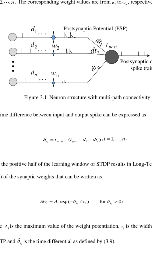
Figure 3.1 Neuron structure with multi-path connectivity ... 42
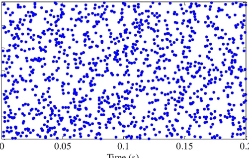
Figure 3.2 Spike raster of input spike trains when N=600. ... 50
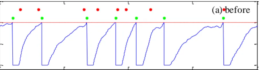
Figure 3.3 Training results without noise (a)Vm: membrane potential after learning; red dots: target spike train; green dots: actual output spike train; (b)correlated-based metric C of target and output spike trains. ... 50
Figure 3.4 Temporal sequence learning of a typical run without noise (a)membrane potential before learning; (b)membrane potential after learning; (c)learning process. ... 51
Figure 3.5 Synaptic weights during CCDS supervised learning ... 53
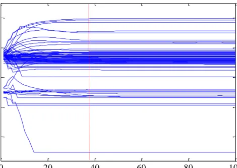
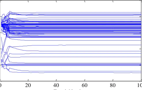
Figure 3.6 Comparison between CCDS and ReSuMe (a)evolution of the weights during CCDS learning; (b)evolution of the weights during ReSuMe learning. ... 54
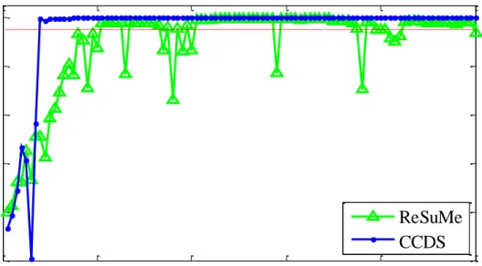
Figure 3.7 Evolution of correlated-based metric C for both ReSuMe and CCDS ... 55
Figure 3.8 Adaptive learning of different target trains (a) sequence learning with the changed target train; (b)Correlated-based metric C of target and output spike trains. ... 56
Figure 3.9 LIF neuron, SRM neuron and Izhikevich neuron are driven by the common set of presynaptic stimuli, and trained on the common target signal. ... 57
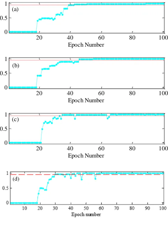
Figure 3.10 Correlated-based metric C of target and output spike trains with (a) LIF neuron; (b) Izhikevich neuron with single spike pattern RS; (c) Izhikevich neuron with two spike patterns RS and IB; (d) SRM neuron. ... 59
Figure 3.11 Temporal sequence learning of a typical run with noise ... 60
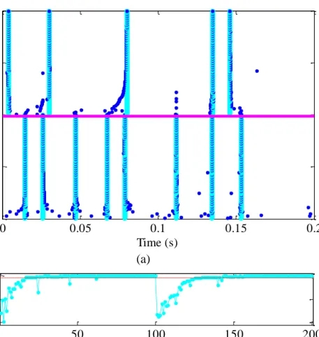
Figure 3.12 Training results with noise Ins=0.2nA. (a) Vm: membrane potential after learning; red dots: target spike train Sd; green dots: actual output spike train So; (b) correlated-based metric C of target and output spike trains. ... 61
xii
Figure 3.14 Spike pattern examples generated for training/testing ... 63
Figure 3.15 Average accuracies for the classification of spatiotemporal patterns using CCDS. ... 63
Figure 3.16 Comparison between CCDS and ReSuMe for (a)different simulation times between 0.25s and 2.5s when Fin= 10 Hz, averaged over 100 runs; (b)
different input frequencies: Fin=10 Hz and Fin=20 Hz withFout=40 Hz and
simulation time T=400ms. ... 67
Figure 4.1 Multilayer structure of feed-forward spiking neural networks with n delayed axonal and synaptic connections, I input layer neurons, H hidden layer
neurons and O output layer neurons. ... 80
Figure 4.2 Encoding of a real-valued feature of 5.4 using Gaussian Receptive Fields neurons ... 87
Figure 5.1 Wavelet Decomposition and Spike Phase Encoding with Two-Stage
Modulate-and-Integrate Module ... 95
Figure 5.2 A schematic representation of procedures for interictal spike detection
problem ... 101
Figure 5.3 Illustration of wavelet encoding for EEG on patient 3 ... 102
Figure 5.4 Interictal spike detection on patient 3 in the first 3 segment (a)raster plot of processed EEG signal with spikes; and (b) detected spikes ... 103
xiii
ABBREVIATIONS AND ACRONYMS
AER Address-Event Representation
ANN Artificial Neural Network
ASNN Artificial Spiking Neural Network
BCM Bienenstock-Cooper-Munro
BSA Bens Spiker Algorithm
BP Back Propagation
CCDS Cross-Correlated Delay Shift
EEG Electroencephalography
ESN Echo State Network
FPGA Field-Programmable Gate Array
GPGPU General Purpose Graphic Process Unit
GRF Gaussian Receptive Field
HH Hodgkin and Huxley
HSA Hough Spiker Algorithm
IB Intrinsically Bursting
ICA Independent Component Analysis
IF Integrate-and-Fire
LIF Leaky Integrate-and-Fire
LOOCV Leave-One-Out-Cross-Validation
LSM Liquid State Machine
xiv LTP Long-Term Potentiation
MAT Multiple-timescale Adaptive Threshold
MuSpiNN Multi-Spiking Neural Network
MutCCDS Multilayer Cross-Correlated Delay Shift
MutReSuMe Multilayer Remote Supervised Method
MutTmptr Multilayer Tempotron
NEST NEural Simulation Tool
ODE Ordinary Differential Equation
PE Phase Encoding
PBSNLR Perceptron-Based Spiking Neuron Learning Rule
PSC Post-Synaptic Current
PSD Precision-Spike-Driven
PSP Postsynaptic Potential
RBF Radial Basis Function
ReSuMe Remote Supervised Method
ROC Rank-Order Coding
RS Regular Spiking
SNN Spiking Neural Network
SPAN Spike Pattern Association Neuron
SRM Spike Response Model
STD Short-Term Depression
STDP Spike Timing Dependent Plasticity
xv
SWAT Synaptic Weight Association Training
VLSI Very-Large-Scale Integration
WBC Wisconsin Breast Cancer
1
1. INTRODUCTION
1.1 Background
Many artificial/ biological systems begin with a small set of abilities, and develop new
abilities through learning and other types of adaptation as time goes on. Artificial Neural
Networks (ANNs) is an important class of machining learning methods inspired by the
features of biological neurons and nervous systems. The research on ANNs has achieved a
great deal in both theories and engineering applications.
Dubbed as the third generation of ANN, Spiking Neural Networks (SNNs) [1], [2] are
considered to be more biologically realistic as compared to the typical rate-coded networks
since they can model more closely different types of neurons and their related temporal
dynamics. Neurons will send out short pulses of energy (spikes) as signals if they have
received enough input from other neurons. Based on this mechanism, spiking neurons are
developed with the same capability of processing spikes as would be expected from
biological neurons. Such biologically plausible construction ensures SNNs a greater
processing power in manipulating temporal signals, and better robustness in complex
patterns learning. Most of the attention of SNNs has been focus on: 1) the design of spiking
neuron model [3], [4]; 2) information encoding method [5]–[7]; 3) training algorithm [8]–
[10]; 4) applications [11]–[13] and 5) hardware implementation [14]–[16].
The learning of ANNs indicates the rules to change the synapse weights, and consequently
2
learning and recall procedure could naturally satisfy the requirements of the temporal
biological data processing and could also provide greater computing power than would be
expected from conventional ANNs learning using smaller networks sizes. SNNs have been
extensively studied in recent years, but questions of how information is represented by
spikes and how the neurons process these spikes remain unclear.
SNNs exhibit interesting properties that make them particularly suitable for applications
that require fast and efficient computation and where the timing of input/output signals
carries important information. Firstly, SNNs are not only adaptive, but also
computationally powerful. Second, the representation of signals transmitted through and
produced by SNNs resembles those required to stimulate the nerves. Moreover, SNNs
possess the ability to learn from examples and are expected to inherit generalization
properties, common to most classes of ANN. SNNs have three main functional components:
encoding, learning and decoding. The choices in terms of encoding method and learning
method depend on the application. Strong evidence suggests that supervised learning
occurs in the cerebellum and the cerebellar cortex [17]. In order to take advantage of the
properties of SNNs, an efficient learning algorithm is desired.
Applications of ANNs have gained increasing interest over the past two decades. Various
tasks has been done successfully, such as pattern and sequence recognition [18]; data
processing [19]; decision making [20]; system identification and control [21]; medical
diagnoses [13]; image/object recognition [22]; autonomous robotics [23]; optical
3
SNN get closer to biological examples, it become possible to emulate part of function of
the biological nervous system to process the information which normally happen in the
brain, but still not clear understood. For instance, utilize SNN into the study of processes
such as: the study of mental illnesses by emulating brain disorders and testing how drugs
affect the brain. When the SNNs is used to analyze brain signals, supervised learning is
required for the SNNs to work as a classifier or a pattern recognizer. The final goal of
studying involving SNN is to understand how the human brain works. However, the
limitations in the existing encoding method and learning rules have thus far restricted the
applications of SNNs. Therefore, improvements on these aspects as proposed here could
broaden the practical implications of SNNs-based systems and their consequential
application in signal processing.
1.2 Research Purpose
This dissertation focuses on developing a biologically plausible information processing
system using SNNs, and its applications on biomedical signals. The specific goal of this
research is fivefold:
1. Developing an integrated consistent system of spiking neurons to perform various
recognition tasks, where the encoding, the learning, and the readout are considered
from a systematic level.
2. Developing a new temporal learning algorithm that is both computational efficient and
4
3. Investigating various properties of the proposed learning algorithm, such as learning in
the presence of noise, generality to different neuron model, adaptive learning
performance, effects of parameters, etc.
4. Investigating the temporal learning in multilayer spiking neural networks.
5. Investigating the ability of the proposed learning rule and neural network structure for
different cognitive tasks, such as interictal spike detection, Iris classification and
Wisconsin Breast Cancer classification problem, etc.
1.3 Methodology
In this work, we applied analytical and computational methods for the following tasks:
1. Our approach is to present a systemic understanding of how pattern encodings might
happen in the nervous system and a learning displays technical capacity. An analytical
method was used to develop what is termed here as a Cross-Correlated Delay Shift
(CCDS) learning rule based on the design principles of the ReSuMe rule. Axonal delays
and synapse delays were integrated to the CCDS rule as an extension of the ReSuMe
learning rule. The delay shift method adapts the actual delay values of the connections
between neurons during training. Input spike patterns close to the synaptic vector will
make the neuron emit an output spike. The proposed learning method is a heuristic
method, which helps the neuron generate output spikes at desired instances and also
tries to remove undesired output spikes. During learning, the output neuron
5
level and produce the desired output. In addition, the total PSP is reduced below the
firing threshold at the instances of undesired output spikes to remove the undesired
spikes. Meanwhile, the cross-correlated term is introduced to speed up the learning
process. The CCDS learning rule was tested with random input temporal spike patterns,
and the output accuracy and computation efficiency is compared to those of the
ReSuMe learning rule as stimulated by the same input.
2. We expanded the structure of weight matrix, axonal delays and synapse delays with the
idea that combining those variables and mapping them into a single higher dimensional
matrix. The proof of concept was done by performing the gradient descent on such
special structured spiking neural network and minimizing network error function
similar to back-propagation of ANN. It combines the quality of SpikeProp with the
flexibility and efficiency of CCDS, i.e., it can be used with multi spikes and different
neuron model in multiple layers in the efficient training process. It improves the
capability of CCDS on classification of nonlinear problems when networks without
hidden layers cannot perform nonlinear operations.
3. We extracted features from EEG records which could help seizure detection by
simulating a specially designed SNN structure with customized neuron models. The
SNNs with several input neurons and one output neuron was implemented to analyze
EEG data with interictal spikes. Each channel of the EEG signals was encoded into
spike trains using recently proposed Wavelet Encoding Device (WED) [7] encoding
6
be generated at the output neuron when epileptic seizures occur. An assessment was
also be conducted on the interictal spikes detection by the template matching algorithm
[25], the feature extraction method using Walsh transform [26], the ReSuMe rule [27]
and the proposed learning method for validation purposes. The entire simulation was
done in the Python interface of the SNN simulation platform together with Matlab
environment.
1.4 Original Contribution of This Dissertation
Neurons in the nervous systems transmit information through spikes (action potential). It
is still unknown that how neurons with spiking features give rise to cognitive functions of
the brain. This dissertation presents detailed investigation on information processing and
cognitive computing in SNNs, trying to reveal how the biological systems might operate
under a temporal framework. The main contribution of this study is threefold:
1. Developed a novel biologically plausible learning rule which has improved learning
accuracy and learning speed in processing and memorizing spatiotemporal patterns. It
reliable in its deployment in the supervised training phase. The learning rule has the
following features:
(i) It enables efficient and effect training of SNN to store and precisely reproduce
spatiotemporal patterns of spikes. Competitive efficiency compared to other
7
(ii) It exhibits generalization properties, i.e., the proposed rule is independent on the
spiking neural models and can be effectively applied to different class of spiking
neurons.
(iii) Robustness against noisy conditions. The functions of delay and noise in neuron
connection is well tested.
(iv) Adaptive to variant spatiotemporal patterns of spikes.
2. Applied the single layer temporal learning rule to the multi-layer network. Comparing
with the multilayer Remote Supervised Method (MutReSuMe) [28] and multilayer
tempotron rule (MutTmptr) [29], Multilayer CCDS (MutCCDS) shows better
generalization ability and faster convergence. The proposed multilayer rules provide
an efficient and biologically plausible mechanism, describing how delays and synapses
in the multilayer networks are adjusted to facilitate the learning.
3. Developed an integrated consistent system of spiking neurons, and applied SNN to
biomedical signal processing. Specifically in this work, we used the spike time
encoding method to extract important features from electroencephalogram (EEG)
records, then utilized the proposed supervised learning rule to analysis and detect the
interictal spikes for patients with epilepsy. By integrating with encoding and learning
function parts, it achieved a reasonably high detection accuracy, i.e., it identified 69
spikes out of 82 spikes, or 84% detection rate. Simulation results show that the applied
8
1.5 Dissertation Organization
This dissertation introduces a novel learning algorithm for implementing ASNN and
applying it to biomedical signal processing. The dissertation is structured into seven
chapters, starting from the current chapter that outlines the research background and
purpose.
Chapter 2 introduces multiple existing models of spiking neurons and synapses, and the
selection criterion for a good neuron model is discussed. The SNN architecture are
overviewed. Existing rate encoding and temporal encoding approaches are also reviewed
in this chapter to provide a retrospective on SNN encoding schemes. Various methods of
unsupervised and supervised learning in SNN are presented at the end of this chapter.
In Chapter 3, a novel temporal learning rule, named Cross-Correlated Delay Shift (CCDS)
learning rule, is developed for learning association of spatiotemporal spike patterns. The
formal definitions of the CCDS learning rule and network architecture for CCDS is
described. Various properties and learning performance are investigated through extensive
experiments. The CCDS rule is able to perform the classification task, but also can
memorize patterns by firing desired spikes at precise time in a faster way than existing
supervised learning methods. It is simple, efficient, yet biologically plausible.
In Chapter 4, the learning in multilayer spiking neural networks is investigated. The
9
multilayer ReSuMe is given. Several tasks are used to analyze the learning performance of
the multilayer network.
Chapter 5 elaborates on the learning rule and network structure, the application of the
CCDS rule to the interictal spike detection in epilepsy patients from EEG records are
presented. A preprocessing unit for the Leaky Integrate-and-Fire (LIF) spiking neurons is
utilized to decompose the input EEG signal into the wavelet spectrum, then further encode
the spectrum amplitude into the delay amount between output spikes and the clock signals.
Empirical results of Phase Encoding (PE) of EEG signals are provided first. The system
architecture and parameters for detection task are described in this chapter, followed by the
detection results and discussions.
Chapter 6 summarizes and discusses the main results of this dissertation, and provides
10
2. SPIKING NEURAL NETWORKS
Spiking neural network (SNNs), termed as the third generation of ANNs, transfer
information in the form of precisely time events called spikes. Spiking neural networks are
biologically-inspired networks that model the behavior of neurons in the brain. Such
networks have a number of advanced properties compared to the traditional rate-based
artificial neural network, the main difference coming from the information transmitted by
time. The basic idea is biologically well found: the more intensive the input, the earlier the
spike transmission, as in visual systems [27]. Discrete spikes and propagation delays are
used to identify temporal patterns. Since the basic principle underlying SNNs is different,
much of the work on traditional neural networks, such as learning rules and theoretical
results of neuron models, has to be adapted, or even has to be rethought. Most popular
neuron models and how to select the appropriate neuron model for a specific application
are described first, then models of synapse and network architecture are summarized. This
chapter also reviews the literature of spiking neurons on existing encoding methods in
determining input signals for SNNs, and temporal learning method for spiking neural
networks.
2.1 Models of Neurons
Neuron models are the elementary units which determine the performance of a SNN. It is
11
potential dynamics of a neuron cell. A lot of spiking neuron models have been emergent in
literature. We only summarize the most popular ones in this section.
Hodgkin-Huxley (HH) model [30]: In 1952, Hodgkin and Huxley modeled the
electro-chemical information transmission of natural neurons with electrical circuits: um is the
membrane potential, Cm is the capacitance of the membrane, gi stand for the conductance
parameter for a specific ion channel (sodium (Na), potassium (K), etc.) and Eiis the
corresponding equilibrium potential. The variable m,hand n describe the opening and
closing of the voltage dependent channels. The dynamic of membrane potential is governed
by the following ODE:
) ( ) )( ( ) )( , ( ) ( Na m Na k m k L m Na all m m I t g m n u E g h u E g u E dt du C . (2.1)
Hodgkin and Huxley model was based on the well-known voltage clamp experiment on
the giant axon neuron found in squid. By analyzing the dynamics of these gating parameters,
the functions gNa and gk are fitted to polynomial functions:
m m m m m m 3 Na Na 4 K K ( )(1 ) ( ) ( )(1 ) ( ) ( )(1 ) ( ) ( ) m m n n h h dm u m u m dt dn u n u n dt dh u h u h dt g g m h g n g n (2.2)
where gNa and gK are the constants of maximum conductance for sodium and potassium
12
from open state to close state, while βm, βn, and βh are the changing speed in the opposite
direction. All these changing speeds are unitless univariate functions that depend solely on
um, with outcome ranges between zero and one. The functions fitted by Hodgkin and
Huxley are: ) 1 ) 10 / ) 30 /(exp(( 1 /20) exp( 07 . 0 ) 80 / exp( 125 . 0 1 ) 10 / ) 10 exp(( ) 10 ( 01 . 0 ) 18 / exp( 4 1 ) 10 / ) 25 exp(( ) 25 ( 1 . 0 m h m h m n m m n m m m m m u u u u u u u u (2.3)
Equations (2.1), (2.2), and (2.3) constitute the original HH model. It is by far the most
detailed and complex neuron model. However, the HH model is less suitable for
simulations of large networks and its applications in ASNN are still rare, due to its large
computational cost.
Integrate-and-Fire (IF) model [31]: and its variants, such as Leaky integrate-and-fire
(LIF) [32], quadratic integrate-and-fire (QIF) [32], exponential integrate-and-fire (EIF) [33]
and generalized integrate-and-fire (gLIF) [34] are simpler than the Hodgkin-Huxley neuron
model and much more computationally tractable. The most important simplification in the
LIF neuron implies that the shape of the action potentials is neglected and every spike is
considered as a uniform event defined only by the time of its appearance. The electrical
circuit equivalent for a LIF neuron consists of a capacitor C in parallel with a resistor R driven by an input currentI(t). The dynamics of the membrane potential in the LIF are
13 ) ( ) ) ( ( 1 t I V t V R dt dV C rest , (2.4)
where V is the membrane potential, spike firing time (f)
t is defined by V(t(f)) with 0 ) ( ( ) ' f t
V . When V is not differentiable, V'corresponds to the left derivative.
The LIF model has been further improved by introducing other biologically plausible
features, such as nonlinear leakage term [35] and moving thresholds [33], [36]. The
variability of thresholds in the moving threshold models equipped the LIF model with a
refractory period, which is argued to be very important in the cognition process of spiking
neural network (SNN) [31], [37]. The multi timescale adaptive threshold (MAT) model
proposed in [4] is preeminent in its accuracy of reproducing the neuron behaviors, which
won the competition of neuronal activity challenge launched by the International
Neuroinformatics Coordinating Facility in 2009 [38].
Izhikevich neuron model: By applying bifurcation methodologies to the HH model,
Izhikevich proposed a two dimensional model [3], [39] recently. It able to reproduce many
realistic neural behaviors, like bursting or single spiking, with different parameter values
in simple equations: m m 2 ( ) 0.04 5 140 all du a bv u dt dv v v u I dt (2.5)
14 if v 30 mV, then v c u u d . (2.6)
The Izhikevich model successfully reproduces different types of neuronal dynamics,
although the conductance and current changes of the ion-channels are not fully described.
It was widely acknowledged by researchers working on large-scale neural network
simulation [40], [41].
Spike Response Model (SRM): as defined by Gerstner et al. [32] in a different way,
expresses the membrane potential Vi of neuron Ni as a time integral over the past,
including a model of refractoriness. The SRM is a phenomenological model of neuron,
based on the occurrence of spike firings.
Let {( ):1 }{ | ( ) '( )0} t u t u t n f t F i i f i
i denote the set of all firing times of
neuron Ni, and i = {
j
|
N
j is presynaptic toN
i} define its set of presynaptic neurons. The state Vi(t) of neuron Ni at timet
is given by
j i f i i f i j t F i f j ij ij F t f i i i t t t w t t r I t r dr V ) ( ) ( current input external if 0 ) ( ) ( ) ( ) ( ) ( ) ( ) (
, (2.7)where the kernel functions i,ij andi respectively describe the potential reset, the response to a presynaptic spike and the response to an external current.
15
E. Izhikevich provided a nice table [39] in 2004 that compares different neuron models in
terms of biophysical meaning, the types of biological neuron behavior that the model is
able to replicate and the number of floating-point operations required for each step of
simulation during a 1ms time span. These neuron models vary from the most complicated
ones fitted to mimic real biological neurons, to the simplest ones, which only abstract the
most important electrophysiology features. However, the challenge remains in selecting a
proper model for the SNN because of the difficulty in balancing accuracy and complexity
of the mathematical model while attempting to reproduce the dynamic behavior of a neuron
model.The HH model and the Izhikevich model have been successfully used in simulating
functional blocks of a biological nervous systems [42], [43] due to their ability to simulate
complicated single neuron activities. The model of a single neuron for building large-scale
brain must be: 1) capable of producing rich firing patterns exhibited by real biological
neurons, yet, 2) computational simple, that is, simple neuron models with few parameters.
However, most applications require large-scale SNN implementation, making phenomenal
models the preferred ones for their simplicity in structure and efficiency in the simulation
process [1]. The LIF model with its plausible biological features has been proven to work
well in biological SNN behavior analysis and computer-aided recognition and
classification tasks [13], [33], [44], [45]. When the computational requirements are
substantial, as in the case of large-scale SNN implementation, the LIF models or even
16
2.2 Models of Synapse
In the nervous system, synapse is a structure or interaction between two neurons with
electrical or chemical signal transmitted from one to the other. Synaptic interaction is a
more complex phenomenon than the neuron dynamics themselves. Thus, few detailed
biophysical synaptic model exist. The most widely used synapse model in computational
neuroscience are the phenomenon model, in which synaptic interactions are modeled by
interaction kernels which sum up linearly over different synapse and time. The total impact
of all synapses can be expressed in the following equation:
k s ) ( ) ( synapses spikes s k k syn t w ε t t f , (2.8)where wk is the weight of the kth synapse and kdenotes its synaptic interaction kernel. The interaction kernel can be an arbitrary shape, but it is constrained by the biophysics of
synaptic interaction in most models. A widely used phenomenological model is as the
following function: ( ) 1 exp( ) exp( ) ) ( fall rise fall rise t t t H A t
, (2.9)where the two exponential functions model the arrival and leaving of neurotransmitters at
the postsynaptic site, governed by time instance rise and fa ll, respectively. H(t) is the Heaviside step function.
17
2.3 Network Architectures
Within the class of computationally oriented spiking neural networks, two main directions
are distinguished. First, use the network structure equivalent to traditional neural networks.
Feed-forward network is the simplest and mostly used network structure for spiking
neurons[28], [52], [53]. Due to the complex dynamic of the spiking neurons, recurrent
structure of spiking neural network is rare investigate[54]. Second, there are uniquely
network structure for networks of spiking neurons. Most famous two network structures
are the Echo State Network (ESN) and Liquid State Machine (LSM), which also called
reservoir computing. Typically an input signal is fed into a fixed dynamical system called
reservoir and the dynamics of the reservoir map the input to a higher dimension. Then a
simple readout mechanism is performed to read the state of the reservoir and map it to the
desired output. For reservoir computing, the training is only performed at the readout stage
and the reservoir is invariant.
Echo State Network [55]: proposed by Jaeger in 2001, was intend to learning time series
) ( ), ( , ), 1 ( ), 1 ( d uT dT
u with recurrent networks. The internal states of the reservoir are
supposed to reflect the concurrent effect of a new teacher input u(t1) and the desired output d(t), related to the previous time. Therefore, there are the backward connections
from the output layer toward the reservoir (Fig. 2.1) and dynamics of the network is
governed by the following equation:
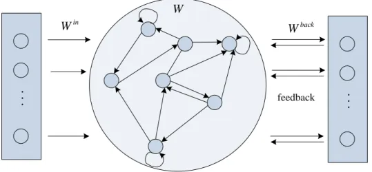
)) ( ) ( ) 1 ( ( ) 1 (t f Winu t Wx t Wbackd t x (2.10)
18 N reservoir units K in p u t u n it s L o u tp u t u n its (r ea d o u t f u n ct io n ) . . . feedback ... in W W back W
Figure 2.1 Architecture of ESN
where x(t1) is the new state of the reservoir, in back
W W
W , ,and are the input weight
matrix, the matrix of weights in the reservoir and the matrix of feedback weights from the
output of the reservoir, respectively.
ESNs have been successfully applied in many experiments, with 20-400 internal units in
the network. Jaeger introduced spiking neurons model, LIF model, in the ESNs, mastered
the benchmark task of learning the Mackey-Glass chaotic attractor [55]. Results improve
substantially over the ESNs using sigmoid units. Verstraeten et al. [56] compared several
measures for the reservoir dynamics with different neuron models.
Liquid State Machine [32]: proposed by Maass, was to explain how a continuous stream
of input u() from the changing environment can be processed in real time by recurrent connections of IF neurons, as shown in Fig. 2.2. The reservoir here works as a liquid filter
19 M
L , operates similarly to water undertaking the transformation from the low-dimensional
space of a set of stimulating surface into a higher dimensional space of waves in parallel.
The liquid states xM(t) are transformed by a readout map M
f to generate an outputy(t).
LSM can be written as the following equations:
) ))( ( ( ) (t L u t xM M (2.11) )) ( ( ) (t f x t y M M (2.12) where M
L is an operator that maps input functions u() onto functions xM(t). The LM
operator can be implemented by a randomly connected recurrent neural network. M
f is
the memoryless readout map that transforms the current liquid state into the machine output.
The readout is usually implemented by one or several IF neurons that trained to perform a
specific task using supervised learning rule.
Figure 2.2 Architecture of LSM M L M
t
)
(
t
x
M ) (t y)
(
u
Liquid Readout20
LSM has been widely applied to nonlinear classification problems, such as XOR[57] etc.
It is convenient for capturing most temporal features of spiking neuron processing,
especially for time series prediction and for temporal pattern recognition.
2.4 Encoding Scheme
In biological nervous systems, a neuron transmits information to others via spike trains
with specific frequency and amplitude. The inputs and output of traditional artificial neuron
models such as threshold perceptions and sigmoidal neurons consider only rate encoding
(coded by frequency) and will result in a loss of information expressed in the form of
precise firing times of spikes. The data from the real-world is extremely dynamic, that
everything changes continuously over time. Understanding the representation of external
stimuli in the brain directly determines what kind of information mechanism should be
utilized in the neural network. The most significant difference between SNN and traditional
neural networks is that information in SNN is represented by spike trains which are a series
of pulses with timings of interests. There are mainly two kinds of interpretations developed
about how information is related to spike trains: 1) the rate encoding, which assumes that
the information is encoded by the counts of spikes in a short time window; and 2) the spike
time encoding which considers information carried at the precise time of each action
potential in the spike train. Although the mechanisms for data representation and analysis
using biologically-inspired neural networks is still under development, there are evidences
show that spike time encoding might be more reliable in explaining experiments on the
21
essential in SNN applications. The followings further present a detailed overview of the
rate code and the temporal code.
2.4.1 Rate Code
Rate code is a traditional coding scheme, which assuming that information about the
stimulus is contained in the firing rate of the neuron. Before encoding external information,
precise calculation of the firing rate is required. Thus neuronal responses are treated
statistically or probabilistically. Mostly, rate encoding consider the spike count within an
encoding window. Any information possibly encoded in the temporal structure of the spike
train is ignored.
The simplest rate encoding is feed an analog signal to a Poisson neuron, which fires output
spikes at probability proportional to its membrane potential. Such an encoding method has
been adopted by Sprekeler et al. [60]. and Keer et al. [61] to analyze the recurrent ASNN
behaviors. Although Poisson neuron model is easy for theoretical analysis, it was rarely
implemented in real-world applications due to its inaccuracy in mapping analog signals to
spike trains. Another rate encoding method, termed Hough Spiker Algorithm (HSA), was
introduced by De Garis et al. [62] in 2000. It de-convolves the input signal into its
individual spike responses, so that the post synaptic potential of the encoded spike train
could be quite similar compared to the original signal. Schrauwen et al. [6] improved this
encoding method by optimizing the de-convolution threshold, introduced a new encoding
method called Bens Spiker Algorithm (BSA). BSA has been used widely as a rate encoding
22
Address-Event Representation (AER) is an asynchronous protocol designed for analog
neural system simulation platforms [66]. It is also referred to as an encoding method by
some researchers [67]–[69]. It encounters of “ON” and “OFF” events in the input signals
are registered by AER to generate corresponding output spikes. The “ON” and “OFF” events in AER indicate the time when a change in the input signal either exceeds a positive
threshold or fall behind a negative threshold. Under such definition, AER could be treated
as a rate encoding method with regards to the derivatives of the input signal. The major
problem of rate encoding methods is that an averaging time window is required for each
sampling of the input signal, which as a consequence limits the temporal resolution of the
encoded signals.
2.4.2 Temporal Code
Temporal coding is a straightforward method for translating a vector of real numbers into
a spike train, for instance, for simulating traditional connectionist models using SNNs.
Precise spike timing as a means to encode information in neural networks is biologically
supported. The temporal encoding is outperform rate-based encoding when patterns within
the encoding window provide the information about the input stimulus that cannot obtained
from spike count. For example, there are evidences show that the populations of neurons
in the primary auditory cortex coordinate the relative timing of their action potentials by
grouping the neighboring spikes in short bursts, without changing the number of firings
per second [70]. Another evidence for precise spike timing coding paradigm is required in
artificial systems is: neuroprostheses for movement control where the precise timing of
23
movement trajectories [71]. Thus, the temporal patterns in spatiotemporal spikes can carry
more information than rate encoding especially in the system where the processing speed
is required to be high. For these reasons, much more attention has been focused on the
development of learning rules for spiking neural networks that utilize a temporal coding
scheme. Potential temporal coding strategies based on the precise timing of spikes are
summarized in the following list:
Time to first spike: under this coding scheme, information is assumed to be encoded in
the latency between the beginning of stimulus and the time of the first spike in the response
neuron.
Rank-Order Coding (ROC): the information is encoded by the order of spikes in the
activities of a neural population according to this coding method.
Latency code: the information is encoded by the relative latency between the neighboring
spikes.
Resonant burst coding: downstream neurons affected by resonance are determined by the
frequency of a burst.
Coding by synchrony: this scheme is assumed the neurons that encode different bit of
24
Phase encoding: Neuronal spike trains could encode information in the phase of a pulse
with respect to the background oscillation. A simple implementation of phase encoding
could be realized by linearly mapping the input signal to the delay of spikes within each
synchronizing period [37].
Population encoding: Temporal receptive fields (Fig. 2.3) and the Cosine squared
function method are the most famous population encoding schemes could also be utilized
for phase encoding to improve the encoding resolution [72], [73]. To be more biologically
plausible, Rumbell et al. [74] introduced a synchronizing method which considered spiking
neurons as phase encoding units instead of performing linear mapping between analog
values and spike delays. As shown in Fig. 2.3, input data a is encoded into temporal
spike-time patterns for the input-neurons encoding this input-variable, using multiple local
receptive fields like Radial Basis Functions. The translation of inputs into relative firing
times is straightforward: the highest stimulated neuron, neuron 2, fires at a time close to
0
t , whereas less-stimulated neurons, as for instance neuron 3, fire at increasingly later times. For a data range [ min, , max]
n n
I
I of a variable n,m neurons were used with Gaussian
receptive files. For a neuron i its center was set to Iminn (2i3)/2{Imaxn Iminn }/(m2)
and width 1/ {Imax Imin}/(m2)
n n
. The learning parameter is chosen by trial and error. With such encoding, spiking neural networks ware shown to be effective for
25
Figure 2.3 Population encoding with 8 overlapping Gaussian receptive fields
2.5 Temporal Learning in SNN
Traditional neural networks have been applied to pattern recognition in various guises. The
best-known learning rules for such networks are of course the class of
error-back-propagation rules for supervised learning and unsupervised learning rues such as Hebbian
learning, or Kohonen self-organizing maps. By substituting traditional neurons with
spiking neuron models, two main directions of learning rules for computationally oriented
spiking neural networks have been developed. One is the development of learning methods
equivalent to or similar to those developed for traditional neural networks. The other one
is development of computational learning algorithms unique for networks of spiking
neurons. Both supervised learning and unsupervised learning rules in the temporal
framework are described in this section. T3 T4 T2 1 2 3 4 5 6 7 8 t =9 t =0 a = *,9,3,6,*,*,*,*
26
2.5.1 Synaptic Plasticity
Synaptic plasticity, also called unsupervised learning, refers to the adjustments of synapses
between neurons in the brain. From the biological aspect of neurons, the changes of
synaptic weights with effects lasting seconds or minutes, are called Short-Term
Potentiation (STP) if the weights are strengthened, while Short-Term Depression (STD) if
the weight values are decreased. On the scale of several hours or even more, the weight
changes are referred to Long-Term Potentiation (LTP) and Long-Term Depression (LTD).
A good review of the main synaptic plasticity mechanisms for regulating levels of activity
in conjunction with Hebbian synaptic modification is given in [76]. There are
neurobiological evidences increasingly demonstrate that synaptic plasticity in networks of
spiking neurons is sensitive to the presence and precise timing of spikes [77]. The
best-known learning paradigm for spiking neural network is Spike Timing Dependent Plasticity
(STDP) induced by tight correlations between the spikes of pre- and postsynaptic neurons,
which is often referred to a temporal Hebbian rule. It relies on local information driven by
back-propagation of action potential through the dendrites of the postsynaptic neuron. For
the computational purposes, STDP is normally modeled in SNNs using temporal window
for adjusting the weight LTP and LTD which are derived from neurobiological experiments.
Different shapes of STDP have been studied in [39].
A winner-take-all learning rule [78] modifies the synaptic weights using a time-variant of
Hebbian learning: the weight of the synapse is increased when the start of the postsynaptic
potential at a synapse slightly precedes a spike in the target neuron; earlier and later
27
time. After learning, the firing time of an output neuron reflects the distance of the
evaluated pattern to its learning input pattern thus realizing a kind of RBF neuron.
2.5.2 Supervised Learning
Supervised learning contributes to the development and maintenance of lots of brain
function. There is strong biological evidence that supervised learning exists in the
cerebellum and the cerebellar cortex [17], [79]. However, the mechanism of supervised
learning in the biological neurons remain unclear [57]. In view of this, research on
supervised learning for spiking neurons and spiking neural networks is still at the early
stage, and many existing learning methods have some weakness [8]. Here, we list some
popular supervised learning rules base on temporal encoding, that it, during a certain
running time, neurons can precisely emit spikes at appointed times through learning.
There are two types of supervised learning methods for SNNs based on temporal encoding,
which are classified according to the number of spikes that need to be controller precisely.
The first type is the single-spike learning, which can control only the firing time of a single
spike. The most straightforward approach to implement supervised learning in spiking
neural networks is as the same method used by Rumelhart et al. [80]: using the gradient
descent on the error of the time difference between the desired output spike train and the
actual output spike train. Different from the traditional artificial neural network, the spiking
neuron’s activation function is not differentiable. Thus, backpropagation-like approach was derived for spiking networks with some additional assumptions. To overcome the
28
linearizing the model at a neuron’s output spike times. The SpikeProp [81] rule has been shown to be capable of learning complex nonlinear tasks in spiking neural networks with
similar accuracy as traditional sigmoidal neural networks, including the archetypal XOR
classification task. SpikeProp and its variants such as QProp [82], RProp [82] have two
major limitations [37], [82], [83] : (1) they do not allow multiple spikes in the output spike
train, and (2) they are sensitive to spike loss, in that no error gradient is defined when the
neuron does not fire for any pattern, and hence will never recover. Although single spike
learning rules have good application capability, networks with only single spike output will
limit the capacity and the diversity of information that they transmit. The Tempotron rule
[84], another gradient descent based approach which is efficient for binary temporal
classification task, encounters these two problems as well. As demonstrated in study [85],
non-gradient-based methods like evolutionary strategies do not suffer from these tuning
issues. However, evolution method is very time consuming which is not suitable for
complex tasks.
Relative to the single spike learning, multi-spike learning methods are more consistent with
the running and information transmitting model of the biological neurons. Due to the
complexity of the learning targets increases significantly, most existing multi-spike
learning methods focus on single spiking neurons or single-layer spiking neural networks.
Temporal learning rules, such as SPAN [86], PSD [22], Chronotron [87], have been
developed to train neurons to generate multiple output spikes in response to a
spatiotemporal stimulus. In Chronotron, both analytically-derived (E-learning) and
29
SPAN rule are based on error function that takes into account the difference between the
actual output spike train and the desired spike train. Their application is therefore limited
to tractable error evaluations, which are unavailable in biological neural networks and are
computationally inefficient as well. The I-learning rule of Chronotron is based on a
particular case of the Spike Response Model, which might have limitations for other
spiking neuron models. In addition, it depends on weight initialization. Those synapses
with zero initial value will not be updated according to the I-learning rule, which will lead
to information loss from afferent neurons. For multilayer perceptron networks based on
various spiking neuron models, performance comparable to SpikeProp is shown. An
evolutionary strategy is, however, time consuming for large-scale networks. Carnell and
Richardson [88] first applied the linear algebra into the learning of time series of spikes by
using the Gram Schmidt projection process to calculate the weight change. However, this
method is not a back-propagation based rule which is only applicable to a single spiking
neuron or single layer of SNN. PBSNLR [89] first transform the supervised learning
problem into a classification problem and solves the problem by using perception learning
method. But it needs many learning epochs to achieve good learning performance when
time step is precise.
ReSuMe [27], referred to as the remote supervised method, is one of the few supervised
learning algorithms that is based on a learning window concept derived from STDP. In the
ReSuMe learning process, the desired or supervisory signal does not directly influence the
membrane potential of the corresponding learning neuron. It is described to be biologically
30
in time. Similar to SPAN and PSD, ReSuMe is derived from the Widrow-Hoff rule [90]. It
combines two processes: one is STDP for strengthening synapses based on input spike
trains and desired output spike train; the other one is anti-STDP learning window for
weakening synapses based on the input spike trains and actual output spike train. Under
remote supervision of instruction neuron, the output neuron can produce a desired output
spike train in response to a spatiotemporal input spike pattern. The results show that
ReSuMe has good learning ability and wide applications. With this method, it also can
reconstruct the target input-output transformations. In [57], the ability of ReSuMe on
sequence learning, classification and spike shifting are discussed. As another supervised
learning rule based on STDP, SWAT (Synaptic Weight Association Training) [24] merged
BCM (Bienenstock-Cooper-Munro) learning rule with STDP. Different from ReSuMe,
SWAT focuses on multilayer SNN rather single neuron or single layer SNN. The SNN uses
a feed-forward topology, in which the hidden layer works as a frequency filter while
frequencies of input and output layers are kept as fixed values.
The common disadvantage of these multi-spike learning methods for spiking neurons is
that the learning efficiency is relative low. When the desired output spike train is relatively
long, the neuron needs to run a relatively long time to make the learning converge. In [57],
it needed around 450 epochs to achieve high learning accuracy when a neuron learned to
emit a spike train of 400ms length using ReSuMe. Thus, it lowers its learning efficiency
and weakens its ability to solve real-time problems. In addition to learning efficiency, the
31
desired output spikes increase to a certain degree, and this limits their ability to solve
complicated tasks.
These disadvantages of the existing methods prompted us to search for supervised learning
32
3. CROSS-CORRELATED DELAY SHIFT SUPERVISED LEARNING
METHOD
This chapter introduces a novel learning algorithm for spiking neurons, called CCDS,
which is able to learn and reproduce arbitrary spike patterns in a supervised fashion
allowing the processing of spatiotemporal information encoded in the precise timing of
spikes. Unlike the Remote Supervised Method (ReSuMe), synapse delays and axonal
delays in CCDS are variants which are modulated together with weights during learning.
The CCDS rule is both biologically plausible and computationally efficient. The properties
of this learning rule are investigated extensively through experimental evaluations in terms
of reliability, adaptive learning performance, generality to different neuron models,
learning in the presence of noise, effects of its learning parameters and classification
performance. Results presented show that the CCDS learning method achieves learning
accuracy and learning speed comparable with ReSuMe, but improves classification
accuracy when compared to both the Spike Pattern Association Neuron (SPAN) learning
rule and the Tempotron learning rule.
3.1 Introduction
Spiking neural networks [1], [2], [91], [92] (SNNs) are considered to be more biologically
realistic compared to typical rate-coded networks as they can model more closely different
types of neurons and their temporal dynamics [93]. SNNs exhibit interesting properties that
33
efficient computation and where the timing of input/output signals carries important
information. Various interesting types of neuron models [1], [91], [97]–[100] have
emerged for building large scale artificial SNNs. SNNs rely on three main functional parts:
encoding, learning and decoding.
Recently, the learning problem in a network of spiking neurons has attracted attention from
a number of researchers. One reason for this interest is that in these networks the learning
process is considered as a realistic model in the biological neural networks. There is strong
biological evidence that supervised learning exists in the cerebellum and the cerebellar
cortex [17], [79]. It is shown that supervised signals are provided to the learning modules
or neural structures in the brain. Several supervised learning algorithms have been
successfully developed for nonlinear benchmark problems. Some of the existing
supervised learning rules, such as SpikeProp [101], QProp [82], RProp [82] use error back
propagation similar to the traditional Neural Networks (NNs). The two major limitations
of these methods and their extensions [37], [82], [83] are that (1) they do not allow multiple
spikes in the output spike train, and (2) they are sensitive to spike loss, in that no error
gradient is defined when the neuron does not fire for any pattern, and hence will never
recover. The Tempotron rule [84], another gradient descent based approach which is
efficient for binary temporal classification task, encounters these two problems as well. As
demonstrated in study [85], non-gradient-based methods like evolutionary strategies do not
suffer from these tuning issues. For multilayer perceptron networks based on various
spiking neuron models, performance comparable to SpikeProp is shown. An evolutionary
34
rules, such as SPAN [86], PSD [22], Chronotron [87], have been developed to train neurons
to generate multiple output spikes in response to a spatiotemporal stimulus. In Chronotron,
both analytically-derived (E-learning) and heuristically-defined (I-learning) rules are
introduced. Both the E-learning rule and the SPAN rule are based on error function that
takes into account the difference between the actual output spike train and the desired spike
train. Their application is therefore limited to tractable error evaluations, which are
unavailable in biological neural networks and are computationally inefficient as well. The
I-learning rule of Chronotron is based on a particular case of the Spike Response Model,
which might have limitations for other spiking neuron models. In addition, it depends on
weight initialization. Those synapses with zero initial value will not be updated according
to the I-learning rule, which will lead to information loss from afferent neurons.
Well known biologically-inspired Spike-timing dependent plasticity (STDP) was observed
through experiments on hippocampal neurons [102] which can induce either long- or
short-term potentiation in synapses based on local variables such as the relative timing of spikes,
voltage, and firing frequency. It shows that postsynaptic firing, which occurred within a
time window of 20ms after presynaptic firing, resulted in weight potentiation; whereas
postsynaptic firing within a time window of 20ms before presynaptic f