A Bi-Criteria Active Learning Algorithm for
Dynamic Data Streams
Saad Mohamad, Abdelhamid Bouchachia, Senior Member, IEEE, and Moamar Sayed-Mouchaweh
Abstract— Active learning (AL) is a promising way to effi-ciently build up training sets with minimal supervision. A learner deliberately queries specific instances to tune the classifier’s model using as few labels as possible. The challenge for streaming is that the data distribution may evolve over time, and therefore the model must adapt. Another challenge is the sampling bias where the sampled training set does not reflect the underlying data distribution. In the presence of concept drift, sampling bias is more likely to occur as the training set needs to represent the whole evolving data. To tackle these challenges, we propose a novel bi-criteria AL (BAL) approach that relies on two selection criteria, namely, label uncertainty criterion and density-based cri-terion. While the first criterion selects instances that are the most uncertain in terms of class membership, the latter dynamically curbs the sampling bias by weighting the samples to reflect on the true underlying distribution. To design and implement these two criteria for learning from streams, BAL adopts a Bayesian online learning approach and combines online classification and online clustering through the use of online logistic regression and online growing Gaussian mixture models, respectively. Empirical results obtained on standard synthetic and real-world benchmarks show the high performance of the proposed BAL method compared with the state-of-the-art AL methods.
Index Terms— Active learning (AL), Bayesian online learning, concept drift, data streams.
I. INTRODUCTION
C
LASSIFICATION has been the focus on large body of research due to its key relevance to numerous real-world applications. A classifier is trained by learning a mapping function between input and predefined classes. In an offline setting, the training of a classifier assumes that the training data are representative and are available prior to the training phase. Once this later is exhausted, the classifier is deployed and, therefore, cannot be trained any further even if performs poorly. This can happen if the training data used do not exhibit the true characteristics of the underlying distribution. Moreover, for many applications, data arrive over time as a Manuscript received November 21, 2015; revised May 26, 2016, September 23, 2016, and September 26, 2016; accepted September 26, 2016. The work of A. Bouchachia was supported by the European Commission under the Horizon 2020 Grant 687691 related to the Project: PROTEUS: Scalable Online Machine Learning for Predictive Analytics and Real-Time Interactive Visualization.S. Mohamad and A. Bouchachia are with the Department of Computing, Bournemouth University, BH12 5BB Poole, U.K. (e-mail: smohamad@ bournemouth.ac.uk, [email protected]).
M. Sayed-Mouchaweh is with École des Mines de Douai, 59500 Douai, France (e-mail: [email protected]).
Color versions of one or more of the figures in this paper are available online at http://ieeexplore.ieee.org.
Digital Object Identifier 10.1109/TNNLS.2016.2614393
stream, and therefore the offline assumptions cannot hold, that is, the characteristics of data streams make it impractical to use offline learning algorithms: 1) data streams are unbounded in size; 2) they arrive at high steady rate; and 3) they may evolve over time. Thus, to deal with data streams efficiently, the classifier must (self-)adapt online over time [1], [2]. To do that, the classifier needs to be fed with labeled data continuously, which is not feasible in most real-world streaming situations where the data are usually unlabeled. It is therefore very important to seek well-informed ways to obtain labels. Active learning (AL) methods provide a systematic approach to select data examples whose labels should be queried. The overall aim of AL is to provide, in the worst case, the same performance as that of passive learning (i.e., relying on random sampling) while using less labeled examples.
For the sake of illustration, consider the example of Internet advert popping up on screen where both online and AL are relevant. The goal is to predict if an advert item will be interesting to a given shopper at a given time. To this end, a classifier is built based on the feedback from the shoppers. However, the interest and preference of the shoppers may change over time leading to what is known as concept drift. Therefore, building a static model for such a scenario will not be effective; hence, the importance of an online adaptive model is manifested. In the streaming setting, obtaining unlabeled data is often cheap but labeling it is expensive. For instance, in the previous example, asking frequently for feedback whether an advert is interesting would annoy the shoppers; hence, AL should be deployed in applications with caution.
AL allows to label, by an expert, some selected data samples according to some selection criteria. Three main approaches of AL have been considered in the literature [3]: membership query synthesis (MQS), pool-based selective sampling (PSS), and stream-based selective sampling (SSS). According to MQS, the learner generates new data samples from the feature space that will be queried. However, labeling such arbitrary instances may be impractical, especially if the oracle is a human annotator as we may end up querying instances [4] that are hard to explain. PSS is the most popular AL method, according to which the selection of instances is made by exhaustively searching in a large collection of unlabeled data gathered at once in a pool. Here, PSS evaluates and ranks the entire collection before selecting the best query. On the other hand, SSS scans through the data sequentially and makes query decisions individually. In the case of data streams, PSS is not appropriate, especially when memory or processing power is limited. It also assumes that the pool of data is stationary and 2162-237X © 2016 IEEE. Personal use is permitted, but republication/redistribution requires IEEE permission.
uses the whole data set. This will delay the adaptation and waste the resources. SSS, instead, adapts the classifier in real-time leading to fast adaptation. Therefore, in this paper, the SSS approach is adopted.
To select the data examples to query, different criteria may be used. Among the most known criteria are label uncer-tainty and density-based labeling [3]. The label unceruncer-tainty (or uncertainty sampling) is a simple and popular criterion and, more important, it is very suitable for online AL. It has been extensively used in both PSS [5], [6] and SSS [7], [8]. Label uncertainty aims at selecting the most uncertain instances that typically lie close to the decision boundary. The training of the classifier on those instances is expected to adjust the boundary, achieving better classification accuracy. That means that the sampling is biased toward the decision boundary of the classifier. However, given the nonstationary aspect of data coming over time in a stream, concept drift can happen any time and everywhere in the feature space. If the drift is close to the current classification boundary, the bias created by AL is not only acceptable, but also desirable. On the other hand, when concept drift occurs far from the boundary, it may go unnoticed. In such a case, the bias is undesirable and it is known as sampling bias problem [9].
On the other hand, density-based labeling selects instances for labeling from highly dense regions in the space, thus representing better the data distribution. It allows covering the whole input space with only few data samples [10] and reducing the sampling bias. Density-based labeling has been applied on offline stationary data in the PSS approach where it is usually combined with label uncertainty [11]–[13]. To the extent of our knowledge, this combination has not been implemented in the SSS approach.
In this paper, we introduce a bi-criteria AL (BAL) algorithm for evolving data streams. In particular, we combine label uncertainty and density-based labeling in an SSS-like setting. The uncertainty of data samples is evaluated using a classifica-tion model, while density of regions is evaluated using a clus-tering model. In general, density criterion performs efficiently with few labeled data, since it samples from maximum-density unlabeled regions. On the other hand, uncertainty criterion tunes the decision boundary after selective sampling from the uncertain regions [11], [13]–[15]. Thus, the density criterion is useful when there is regularity in the data, which is the case of many applications. However, the density criterion alone would not provide an accurate classifier. In other words, the density criterion helps establishing the initial decision boundary, while uncertainty sampling "fine-tunes" that boundary by sampling the regions where the classifier is least certain. By combining both criteria, we can take advantage of the density criterion to reduce the data examples required by the uncertainty criterion to build an accurate classifier.
To ensure enough flexibility of BAL, we explicitly distin-guish between the learning engine and the selection engine. The learning engine uses a supervised learning algorithm to train a classifier on the existing labeled data, while the selection engine selects influential samples from the data stream for labeling. Here, the selection engine includes a classifier, which is different from the classifier used by the
learning engine and the clustering model that serves to design and deploy the two criteria.
AL presents an interesting opportunity to handle concept drift by querying the data samples representative of this drift (i.e., its characteristics). In contrast to standard concept drift handling techniques, where only automatic detection mecha-nisms are applied, AL assumes that an oracle provides the truth labels of data. To this end, we use the importance weighting principle to weight labeled data samples that drives a drift in order to increase the importance of their regions in the feature space. The importance weighting principle has also been theoretically proved to correct sampling bias [16]. The BAL algorithm proposed in this paper is the first AL algorithm that is concept drift aware.
To illustrate how BAL behaves, consider the example that pertains to Internet advertisement. Using uncertainty criterion only would result in querying adverts for which the classifier is uncertain, and therefore, by interactively labeling such adverts, the classifier can improve its performance toward a better pre-diction of what to propose to the shopper. On the other hand, the density criterion considers the similarity of the adverts. Thus, from a dense group of similar adverts, only one that represents the whole group will be queried. Clearly combining the two criteria allows querying representative adverts for which the algorithm is not sure. Furthermore, in the streaming case, the interest and preference of the shoppers may change over time; hence, when the change (drift) occurs in relation to those adverts for which the classifier is certain, the sampling bias caused by the AL will be harmful. By implementing the weighting mechanism, we aim at reducing the sampling bias by labeling more of data samples that drive the drift and that make the uncertainty criterion less important for these data.
In a nutshell, our contributions are as follows.
1) We propose a novel online AL algorithm for data streams using a probabilistic model that combines two querying criteria: uncertainty and density-based criteria. To the best of our knowledge, this is the first approach based on density-uncertainty to the online setting. 2) The proposed combination applies classification through
logistic regression and clustering through growing Gaussian mixture models (GGMMs) to implement the two querying criteria in a uniform probabilistic way. The choice of these algorithms is, therefore, genuine. 3) We propose mechanisms to make the BAL algorithm
aware of concept drift. It is the first study that shows the effectiveness of AL in dealing with concept drift. The rest of this paper is organized as follows. Section II presents the related work. Section III describes the proposed selection criteria along with the classification and clustering algorithms used. Section IV provides the details of the online sampling method proposed before the BAL algorithm is pre-sented in Section V. Section VI discusses the experimental results for a number of well-known synthetic and real-world data sets. Finally, Section VII concludes this paper.
II. RELATEDWORK
AL for online stationary data with no concept drift has been the subject of a number of studies [17], [18]. However,
the approaches proposed in these studies do not meet the requirements of evolving data streams. They are not equipped with mechanisms that enable them to perceive changes of the data distribution and, therefore, ignore the samples of great value that help improve the learner accuracy. In the case of concept drift, they tend to react to changes occurring far from the decision boundary only slowly, hence the problem of sampling bias. However, they may well handle drift that happens gradually and close to the boundary.
Online AL methods for data streams in the presence of drift have been dealt with using batch-based learning, where data are split into batches [19], [20], which are used to adapt the classifier. These methods often assume that the data are stationary within each batch, where pool-based AL strategies are applied. Lindstrom et al. [21] use a sliding window approach, which discards the oldest instances instead of explicitly detecting the changes. Label uncertainty is then used to label the most representative instances within each new batch. In contrast, our online AL handles concept drift directly online by evaluating data instances on-the-fly, allow-ing faster adaptation as soon as drift is detected. In [22], an online approach was compared against a batch-based approach using a fixed and a variable size batch and was found that both have similar accuracy, but the batch-based one required more resources. Another issue is that, in general, batch-based approaches cannot learn from the most recent examples until a new batch is complete. That leads to more delay when responding to concept drift. In online AL, this delay has a negative effect leading to late recovery from drift. For all these reasons, online learning is suitable for dealing with drift compared with batch-based learning.
The closest method to ours is proposed in [7], where online AL is investigated. Authors use randomization to avoid bias estimation of the class conditional distribution that may result from querying. This randomization is combined with the stationary online label uncertainty criterion to deal with drift. They use the notion of budget (i.e., the maximum proportion of instances to be queried over time) to control the resources for labeling. This AL method differs from our BAL approach in at least two aspects. First, the former wastes the resources by randomly picking data in order to cover the whole input space. We, instead, use a density-based criterion, which reduces the sampling bias by sampling from influential (dense) regions. Second, randomization does not have any interaction when drift occurs, and it naively keeps querying randomly as if nothing had happened. In contrast, BAL increases the impor-tance of the drifting regions, thus speeding up the recovery and saving the resources. In Section VI, the superiority of the proposed BAL approach is empirically shown.
III. ONLINEBI-CRITERIAAL
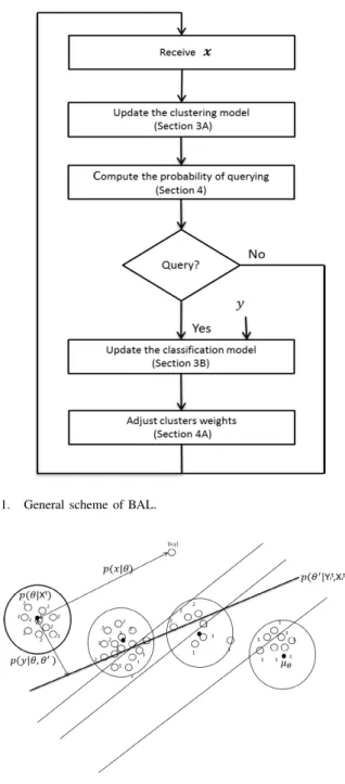
To facilitate the description of BAL, Table I presents the list of symbols used in the rest of this paper. Vectors are bold. The steps of the BAL algorithm proposed in this paper are portrayed in Fig. 1 and the corresponding details are discussed in Section V. In a nutshell, BAL consists of four steps. In the first step, given an instance x, GGMM, used to implement the density-based criterion, is updated (see Section III-A). In
TABLE I TABLE OFNOTATIONS
the second step, using BAL’s sampling model, the probability of querying is computed and the decision whether to query or discard the instance and receive a new one is made (see Section IV). In the third step, the label of the queried instance
x is received and the classification model that is used to
implement the label uncertainty criterion will be updated (see Section III-B). In the fourth step, a weighting technique is used to curb the sampling bias (see Section IV-A).
In order to identify the data examples to query, we seek to minimize the current expected error, which conse-quently leads to the minimization of the future expected error. The current expected error for an instance x can be computed using density-based and label uncertainty criteria, which are estimated by dynamic classification and clustering models.
In [23], it is suggested to select samples that minimize the expected future classification error given as follows:
R=
x
Fig. 1. General scheme of BAL.
Fig. 2. Combining clustering and classification for AL.
where y is the true label of data instance x and y is theˆ predicted output. E[.|x]denotes the expectation over p(y|x). This integral cannot be computed due to its complexity. Nguyen and Smeulders [12], who proposed an AL method that relies on an offline PSS setting, noted that instead of selecting data that produces the smallest future error, we can select the data that have the largest contribution to the current error in order to achieve a good approximation. Another issue pointed out is that the data distribution p(x)affects the expected error. In this paper, we are concerned with online learning. There-fore, in order to have online approximation of (1), an online learning model that involves the online sampling technique is needed. This model should be able to handle real drift and virtual drift [24]. The former refers to changes in the conditional distribution p(y|x), whereas the latter refers to the changes in the distribution of the incoming data p(x).
Our approach deals with the problems mentioned above and works independently of the classifier by adopting an online selection engine that uses the Bayesian inference. The random vector z is typically estimated from a training set of vectors Z [25], [26]. The Bayesian inference estimation process is given as follows:
p(z|Z)=
p(z, |Z)d=
p(z|,Z)p(|Z)d. (2)
Assume that the selection engine has processed until time t, Xt data, among which Xlt are labeled. Ylt is the set of labels associated with Xlt. Replace z with (x,y), Z with (Xt,Ylt), and with(θ,θ), where θ and θ represent the parameters that govern, respectively, the clustering and the classification models. Equation (2) can be written as follows:
px,y|Ylt,Xt = θ θ p(x,y|θ,θ )pθ,θ|Yt l,X t dθdθ (3) pθ,θ|Ylt,Xt = pθ|Ylt,Xt,θ pθ|Ylt,Xtl . (4)
Assuming thatθ andθ are independent, (4) can be rewritten as follows:
pθ,θ|Ylt,Xt= p(θ|Xt)pθ|Ylt,Xlt. (5) Assuming also that all the information about the class label y is encoded in the cluster parameter vector θ, y and x are conditionally independent givenθ. Therefore
p(x,y|θ,θ)= p(y|x,θ,θ)p(x|θ,θ)
= p(y|θ,θ)p(x|θ). (6) Equation (3) can then be rewritten as
px,y|Ylt,Xt = θ θ p(y|θ,θ )pθ|Yt l,Xtl px|θp(θ|Xt)dθdθ. (7) This clearly explains how the selection engine consists of two models: a supervised learning classifier, which is used to estimate the uncertain data examples, and an unsupervised clustering model, which is used to estimate the dense regions. These two models are used to approximate the future error. Equation (1) can be written as follows:
x
y
(yˆ−y)2p(x,y)d yd x (8) p(x,y)can be estimated using (7). This later shows how label uncertainty and density-based criteria are combined. The data examples that minimize the current expected error are those located close to the center of clusters near the class boundaries. Fig. 2 shows an example in two dimensions space, illustrat-ing the relationship between the clusterillustrat-ing and classification models expressed in (7). The distribution of θ and θ are represented by lines and clusters. p(y|θ,θ) depends on the distance between clusterθ and lineθ. p(x|θ)depends on the distance between x andθ. As data are drawn from potentially changing distribution,θ andθ may change.
In the following, the models exploited to implement the two selection criteria are introduced. These criteria are label uncer-tainty defined through logistic regression [27] and density-based criterion defined through GGMM [1].
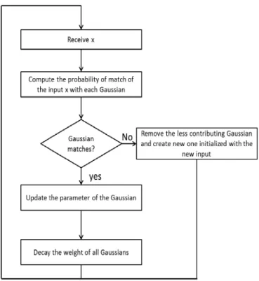
Fig. 3. Main steps of GGMM.
A. Growing Gaussian Mixture Model
To detect the dense regions, an online learning algorithm to estimate the density of data examples xt is needed. According
to Bayesian inference p(xt|Xt−1)=
θt−1
p(xt|θt−1)p(θt−1|Xt−1)dθt−1 (9)
where t represents the time. Traditionally, computing the integral in (9) is not always straightforward and the Bayesian inference is often approximated through maximum-a posteri-ori (MAP) or maximum likelihood estimation (MLE). In order to obtain an online approximation for (9), an online GMM algorithm is used. The GMM perceives the data as a popula-tion with K different components where each component is generated by an underlying probability distribution [28]
p(xt|Xt−1)= K i=1 pxt|θˆti−1 τi t−1 (10)
whereτti−1is the weight of the i th Gaussian,θˆt =(θˆ1t, ...,θˆtK),
whereθˆti is the parameter vector of cluster i .
In this case of incomplete data, MLE and MAP estimates are not directly computable. Therefore, it is standard to use iterative algorithms such as expectation maximization. To accommodate online learning, the GGMM proposed in [1] is adopted. It estimates θˆt from data by maximizing the
likelihood of the joint distribution p(Xt,θˆt) [29]. GGMM
learns from labelled and unlabeled data and handles the complexity of the mixture model efficiently. By using the GGMM, we wish to implement the density-based AL criterion in an efficient way.
The parameters of GGMM are the clusters variance, the learning rate, which determines the update step of the clusters’ parameters, the maximum admissible number of clusters, and the closeness threshold, which controls the creation of new clusters. GGMM creates a new cluster when the Mahalanobis distance between a new input and the nearest cluster is more than the closeness threshold. To make the experiments easier, the closeness threshold is set equal to the variance. GGMM uses a constant fading factor (learning rate) to tune the contribution of clusters by updatingθˆi. The least contributing
clusters are discarded systematically and new ones are added dynamically over time. Fig. 3 shows the main steps of GGMM. Due to its incremental nature, GGMM can cope with concept drift [1] and its combination with the online classifier, logistic regression, (see Section III-B) to devise BAL ensures real-time adaptation.
B. Logistic Regression
To sample the uncertain data examples, the logistic classi-fier, which is offline, probabilistic, and linear in the parameters, is applied. To meet the online requirement of our approach, this classifier will be adapted as will be shown below.
Logistic regression corresponds to the following binary classification model:
y|x∼Bern(μ) (11)
y|x has the Bernoulli distribution with parameterμ given as
μ= p(y=1|x,θ)=sigm(θTx) (12) where sigm(a) refers to the sigmoid function, sigm(a)=(1/(1+exp(−a))).
While in this paper, binary classification is considered, it is easy to extend the logistic regression to multi-class classification. In the following, we discuss the adaptation of logistic regression to online classification and show how it is used in our method for handling concept drift.
1) Bayesian View of Online Logistic Regression: Logistic regression can be trained in an online mode either by using stochastic optimization or by adopting a Bayesian view, which has the obvious advantage of returning posterior instead of just point estimate. In this paper, we use the Bayesian view because we want to capture the nondeterministic nature (uncertainty) of the querying process that itself exploits the label uncertainty criterion. The Bayesian approach of the logistic regression is expressed through
pθtDt∝ pxt,ytθt
pθtDt−1 (13) where Dt is the labeled data seen up to time t. Suppose that at time t −1, our knowledge about the parameters θt−1 is summarized by the posterior distribution p(θt−1|Dt−1). After receiving an observation xt, we consider the probability
pytxt,Dt−1 = θ t pytxt,θt pθtDt−1dθ t (14)
where p(θt|Dt−1) is the predicted posterior, which can be expressed as pθtDt−1= θ t−1 pθtθt−1pθt−1Dt−1dθ t−1. (15)
In order to calculate the expression p(θt|θt−1), we must
spec-ify how the parameters change over time. Following [27], we assume no knowledge of the drifting distribution p(θt|θt−1). Thus, (15) can be eliminated by estimating p(yt|xt,Dt−1),
which is done as follows: p(yt|xt,Dt−1)= θ t−1 pytxt,θt−1 pθt−1Dt−1dθ t−1. (16) Here, two challenges need to be dealt with.
1) Predicting the class of the new data example xtby
com-puting the posterior predictive distribution [see (16)]. 2) Updating the posterior distribution p(θt|Dt)as soon as
the label of xt is obtained by computing [see (13)].
Both challenges require to approximate the prior distribution over the weightθtas a Gaussian distributionN(μt,t). Two
methods have been proposed in the literature to approximate the integral of (16): Monte Carlo approximation and probit approximation [30]. We use probit approximation as it does not require sampling; thus, it takes less computational time. However, it has been found that probit approximation gives very similar results to the Monte Carlo approximation [30]. The result of the approximation is as follows:
p(yˆt =1|xt,Dt−1)≈ ˆ∇t =sigm(K(st)a¯t) (17) st2= xtTt−1xt (18) ¯ at =μt−1Txt (19) K(st)= 1+πs 2 t 8 −1 2 . (20) For more details about the approximation steps, the interested reader is referred to [30].
In the following, we show how the parameters of the pro-posed online logistic regression classifier are updated. We use Newton’s method as formulated in [31] to sequentially update
θ
t =(t,μt)of (13) using (17). Therefore, the meanμt and
covariancet can be updated as follows:
t =t−1−
ˆ∇t(1− ˆ∇t)
1+ ˆ∇t(1− ˆ∇t)st2
(t−1xt)((t−1xt))T
μt =μt−1+txt(yt− ˆ∇t). (21)
These recursive equations reflect on the current and the past data. Nevertheless, the effect of data is implicitly decreasing as more data are processed due to the variance shrinkage.
2) Handling of Concept Drift: In nonstationary setting, a variant version of (21) proposed in [27] is used. The situation is exactly the same as for the stationary case, except that the prior distribution is now N(μt−1,t−1+vtf). Here,
f = c I with c is a constant and I is the identity matrix.
vtf assumes that the weight vectorθt changes are of similar
magnitude. Alternatively, one could use a separate forgetting matrix parameter for every weight coordinate as discussed
in [32]. In this paper, we consider the first assumption
t =(t−1+vt f)− ˆ∇
t(1− ˆ∇t)
1+ ˆ∇t(1− ˆ∇t)st2
×[(t−1+vt f)xt][(t−1+vtf)xt]T
μt =μt−1+txt(yt− ˆ∇t) (22)
where st2 = xTt (t−1+vt f)xt. Here, vt can be thought of
as the Bayesian version of the window size in batch learning for data stream. In order to adjust the model as soon as it becomes unable to estimate the true changingθ distribution, we compute the discrepancy between the predictive class uncertainty after and before observing the true class label
Gt = ˜U(xt)− ˆU(xt) (23)
whereUˆ(xt)is the uncertainty of the label predicted from xt
andU˜(xt)is the uncertainty remaining after incorporating the
true class label ˆ
U(xt)= E[(yˆt−yt)2|xt]
˜
U(xt)= E[(y˜t−yt)2|xt] (24)
ˆ
yt is the predicted label and yˆt = ½(ˆ∇t > 0.5). y˜t is the
predicted label after updating the classification model with the true label. y˜t =½(˜∇t >0.5), where ˜∇ can be computed
as follows: p(y˜t =1|xt,Dt)≈ ˜∇t =sigm(K(s˜t)a˜t) (25) ˜ st2 =xtTtxt (26) ˜ at =μtTxt (27) K(s˜t)= 1+πs˜ 2 t 8 −1 2 . (28) The discrepancy Gt of the model uncertainty is monitored
using a forgetting technique [33]
vt = αvt−1+max(Gt,0)
N Lt
(29) N Lt =αN Lt−1+l(xt) (30)
NLt is the prequential number of labeled data. l(xt)is 1 if xt
is labeled and 0 otherwise.αis a fading factor empirically set to 0.9. Equation (29) will be used to update (22).
Finally, the logistic regression classifier is incrementally updated using (22) that addresses concept drift.
IV. ONLINESAMPLING
In the following, the sampling method used by BAL that avoids the problem of sampling bias is illustrated. Next, a technique to restrict the available resources in terms of labeling budget is described.
We noted earlier that the computation of the future error in (1) is difficult. So instead, we select the sample that has the largest contribution to the current error. Although this does not guarantee the smallest future error, there is a good chance for a large decrease in error. In the offline setting, the selection
criterion based on the set of unlabelled data Du is x =arg max xj∈Du E[(yˆj−yj)2|xj]p(xj) (31) E[(yˆj−yj)2|xj] = p(yj =1|xj)(yˆj−1)2+p(yj =0|xj)yˆ2j (32) where p(y|x) is unknown and needs to be approximated. Nguyen and Smeulders [12] use the current estimation p(y|x,θˆ) assuming that θˆ is good enough. Unfortunately, in the online learning setting, the task is more challenging for three issues.
1) No access to the already seen unlabeled data.
2) The probability p(y|x,θˆ)dynamically changes as more labeled data are seen. That means the approximation assumed above needs adjustment.
3) Need to address the problem of sampling bias (which is detailed in Section IV).
To address these issues, we formulate the querying (sam-pling) probability in a recursive manner as follows. Let q be the binary random variable that determines whether x should be queried. The querying probability is defined by the following model:
q|x ∼Bern(μ). (33) Using (8), the querying probability can be reformulated as follows:
p(q =1|x)=
y
(yˆ−y)2p(x,y)d y. (34) That is to say, a sample that has a large contribution to the current error is likely to be queried.
Now, let us see how this probability is formulated for the online setting, so that we avoid the requirement to have access to the whole data. Let Bt =(Ylt,Xt)be the set of labeled data seen so far. Using (7), we express the probability of querying
xt as follows: p(qt =1|xt,Bt−1)= yt θt ((yˆt−yt)2p(yt|θt,Dt−1)p(xt|θt) p(θt|Xt)dθtdyt) = θt E[(yˆt−yt)2|θt]p(xt|θt)p(θt|Xt)dθt. (35) E[.|θt] denotes the expectation over p(yt|θt,Dt−1).
Using (10), p(qt = 1|xt,Bt−1) can be estimated as
follows: p(qt =1|xt,Bt−1)= K i=1 E (yˆt−yt)2θˆti pxtθˆti τi t (36)
where E[(yˆt−yt)2|θˆti] = ˆU(θˆti)can be computed as
ˆ Uθˆti= p(yt=1|μθˆi t,D t−1)(ˆ yt−1)2 +p(yt =0|μθˆi t,D t−1)ˆ yt2 (37) where μθˆi
t is the mean of cluster i at time t. p(yt =
1|μθˆi t,D
t−1) can be computed using (17) after replacing x
t
by μθˆi
t. The resulting p(yt = 1|μθˆti,D
t−1) is the recursive approximation of the querying probability.
A. Tackling the Problem of Sampling Bias
In general, the AL model starts by exploring the environ-ment. As training proceeds, the model becomes more certain. Then, data samples are queried based on their informativeness. As a result, the training set quickly will no more represent the underlying data distribution, hence the problem sampling bias. Given a classification model with a parameter vector θ, MAP estimate is yˆ = argmaxyp(y|x,θ) and the risk
associated is expressed as R(θ)= x y L(yˆ,y)p(x,y)d yd x (38) where L(.) is the loss function measuring the disagree-ment between prediction and the true label. Since p(x,y) is unknown, the expected loss can be approximated by an empirical risk ˆ Rn(θ)= 1 n n j=1 L(yˆj,yj) (39)
where(xj,yj) are drawn from p(x,y)and n is the number
of samples. In AL, instances are drawn according to an instrumental distribution g(x). Thus, (xj,yj) are sampled
from g(x)p(y|x). In the presence of drift, g(x) may have low probability for data located far from the class bound-ary, because it is considered as an uninformative region. If a drift occurs in that region, many instances with high loss L(yˆj,yj) will not be queried. This leads to a negative
effect of AL; sometimes, worse than learning from random sampling. In order to develop an unbiased estimator of the expected loss, we weight each drawn instance following the concept of weighted sampling. Thus, the empirical risk can be written as follows: ˆ Rg,n(θ)= 1 S n j=1 SjL(yˆj,yj) (40)
where Sj = ((p(xj))/(g(xj))) is the importance weighting
compensating for the discrepancy between the original and instrumental distributions, and S=nj=1Sj is the normalizer.
Thanks to the importance weighting, (40) defines a consistent estimator [34], that is, the expected value of the estimator
ˆ
Rg,n(θ) converges to the true risk R(θ) for n → ∞.
The importance weighting was used in [16] to correct the sampling bias showing that by weighting the queried sample according to the reciprocals of the labeling probability, a statistical consistency is guaranteed. For any distribution and any hypothesis class, AL eventually converges to the optimal hypothesis in the class. In the case of online learning, the importance weighting can be defined as follows:
St = p(xt) p(xt)p(qt =1|xt,Bt−1) = 1 p(qt =1|xt,Bt−1). (41) In order to apply the importance weighting, we interpolate the effect of weighting into the selection engine through the density estimation. Thus, the clustering model is updated with
the importance sampling St. The effect of St on each cluster is represented by Hti as follows: Hti = ⎧ ⎪ ⎨ ⎪ ⎩ St−1p ˆ θi txt , if xt is classified correctly 0, if xt is not queried 1−S−t 1 pθˆtixt , otherwise. (42) Therefore, the new cluster weight can be written as follows:
τi t,St = 1−Hti τi t(1−It)+ 1−Hti τi t +Hti It (43)
where It = | ˆy−y|, that is, It is 0 if xt is correctly classified
and 1 otherwise. The first term of (43) is used to decrease the effect of oversampling by reducing the weight of clusters representing the instances correctly labeled. The second term is used to decrease the effect of undersampling by increasing the weight of clusters representing the instances wrongly labeled.
B. Budget
Under limited labeling resources, a rationale querying strat-egy to optimally use those resources needs to be applied. To this end, the notion of budget was introduced in [7] in order to estimate the label spending. Two counters were maintained: the number of labeled instances ut and the budget spent so
far: bt =((ut)/(|data seen so far|))=((ut)/(|Xt|)). As data
arrives, we do not query unless the budget is less than a constant Bd and querying is granted by the sampling model. However, over infinite time horizon, this approach will not be effective. The contribution of every label to the budget will diminish over the infinite time and a single labeling action will become less and less sensitive. Zliobaite et al. in [7] propose to compute the budget over fixed memory windowsw. To avoid storing the query decisions within the windows, an estimation of ut and bt was proposed. It is computed as follows:
ˆ bt = ˆ
ut
w (44)
whereuˆt is an estimate of how many instances were queried
within the lastw incoming data examples ˆ
ut =(1−1/w)uˆt−1+labelingt−1 (45) where labelingt−1 = 1 if instance xt−1 is labeled, and 0 otherwise. Using the forgetting factor(1−1/w), we showed thatbˆt is unbiased estimate of bt.
In this paper, this notion of budget will be adopted in BAL, so that we can assess it against the AL proposed in [7]. Note that in our experiments in relation to the budget, we set
w=100 as in [7].
V. ALGORITHM
Having introduced the AL criteria and the sampling tech-nique based on Fig. 2, the full details of the algorithm are provided in Algorithm 1. The lines 7, 15, and 16 are included in BAL only when the budget is considered. Otherwise, BAL is not constrained by the budget.
Algorithm 1 Steps of BAL
1: Input: data stream, parameters of GGMM: {maximum
number of clusters, variance, learning rate }, BAL forget-ting matrix f Eq. (22), budget Bd.
2: initialize: t = 0, μ0 = 0, 0 = 5 I Eq. (22), vt = 0 Eq. (29),uˆ1=0 Eq. (45) 3: while (true) do 4: t ←t+1, 5: Receive xt
6: Update the clustering model{θˆt1−1, ...θˆtk−1}by xt.
7: if bˆt <Bd
Eq. (44) then
8: compute μ = p(qt = 1|xt,Bt−1) that refers to the
combination of uncertainty and density criteria using Eq. (36) 9: qt ∼Ber n(μ) Eq. (33) 10: if qt =1 then 11: yt ←quer y(xt)
12: Update the classifier model{μt−1,t−1}by(xt,yt)
using Eq. (22)
13: Remove the effect of sampling bias using Eq. (43)
14: end if 15: end if 16: Computeuˆt+1 Eq. (45) 17: end while
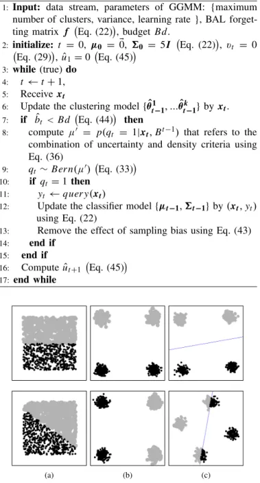
Fig. 4. Synthetic data. (a) Gradual drift (moving plane). (b) Abrupt drift. (c) Mixture drift (moving Gaussian).
VI. EXPERIMENTS
First, BAL is evaluated by analyzing its behavior under different data distributions and different types of concept drift. In order to have controlled settings with known distribution and drift type, 2-D synthetic data sets proposed in [35] are considered. Second, BAL is compared against the state-of-the-art AL methods designed for data streams on real-world data sets. Two real-world benchmark data sets are used: Electricity [36] and Airline [37].
The forgetting constant “c,” which determines that the forgetting matrix f in (22) is empirically set to 5. The parameters of GGMM are empirically specified in Table II. To capture the real performance of BAL, all experiments are repeated 30 times and the results are averaged.
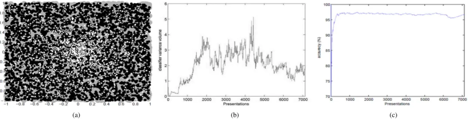
Fig. 5. UAL gradual drift. (a) Data. (b) Classifier variance. (c) Accuracy.
TABLE II
CLUSTERINGPARAMETERS(EMPIRICALLYOBTAINED)
A. Simulation on Synthetic Data
The main goal of this section is to analyze BAL in terms of effect of concept drift and data distribution. Also the impact of the budget and the number of clusters on the performance of BAL are studied. Then, its strengths and weaknesses are discussed. Note that the online logistic regression algorithm serves as learning engine. Three synthetic data sets involving two different distributions, Gaussian and uniform, and three types of data drift, gradual, abrupt, and mixture involving both gradual and abrupt drifts are used. These types of drift occur in real-world applications as shown in the following.
a) Gradual Drift: It considers two sources with grad-ual changes from one source to the other. The so-called moving plane data are used. A gradual changing environment is simulated by rotating the linear class boundary about the origin in a 2-D space. All data points come from a uniform distribution in the unit square [see Fig. 4(a)]. The class definition (concept) changes with each new data point by rotating the boundary at a further angle of 1. The distribution p(x) does not change over time, while p(y|x) does. A real example is when a device begins to malfunction; the quality of its service starts to decrease. After a certain period of time, the device starts to work under failure operation conditions [38].
b) Abrupt Drift: It considers many data sources, each related to one of the target concepts. In the case of abrupt drift, usually one data source is instantly replaced by another. We use four Gaussian sources with half related to one concept and half to another to illustrate abrupt drift. In the substitution process, one data source is instantly replaced by another, yielding a change in p(y|x) with the same p(x) [see Fig. 4(c)]. A real example is the stuck-on or stuck-off faults in a valve or the failed-on or failed-off of a pump [38]. We also
introduce remote abrupt drift for uniformly distrib-uted data by instantly moving the boundary far away (see Fig. 12).
c) Mixture Drift: It is another version of Gaussian drift called moving Gaussian, where both p(x) and p(y|x) change. If p(x)gradually changes, then p(y|x)abruptly drifts and continues gradually drifting [see Fig. 4(c)]. Consider, for example, textual news arriving as a data stream. The goal is to predict if a news item is interesting to a given reader at a given time. The preferences of the reader (P(y|x)) and the news popularity ( p(x)) may change gradually or abruptly over time.
1) Results: The notion of budget is not used here; thus, there is no restriction on the use of resources. In order to study the behavior of BAL on different types of drift and distributions, each data set is experimented using only the uncertainty criterion (UAL). Then, another three experiments on the same data sets are carried out using BAL. Compar-ing the results allows us to study the impact (interest) of incorporating density-based criterion on different scenarios (different distributions and types of drift). The behavior of BAL is analyzed in terms of sequential querying probability and accuracy. In the following, the results of the experiment on these three data sets are shown.
Figs. 5 and 6 show the results after applying UAL and BAL on the moving plane data to test the gradual drift. Figs. 5(a) and 6(a) show the queried data in white. BAL and UAL algorithms adaptively pick the uncertain data around the center of the whole data as the rotation hyperplane crosses the data in the center. However, it is clear that the number of queried data examples using BAL is larger. Figs. 5(b) and 6(b) show the determinant of the variance t computed by (22).
The variance is proportional to the classifier uncertainty. In particular, Figs. 5(b) and 6(b) show that the predictive model uncertainty is fluctuating over time. This fluctuation reflects the continuous data drift, which proves the capability of the classifier to adapt to the gradual drift. Higher uncertainty of the predictive model in Fig. 6(b) implies slow adaptation to drift. It is mainly caused by the uniform distribution of the data leading to inaccurate clustering, that is, the uncertainty criterion alone could be more valuable than its combination with the density criterion. Figs. 5(c) and 6(c) show the accuracy over time. BAL uses more resources to approach
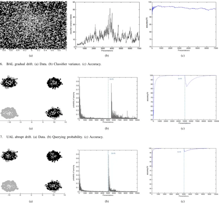
Fig. 6. BAL gradual drift. (a) Data. (b) Classifier variance. (c) Accuracy.
Fig. 7. UAL abrupt drift. (a) Data. (b) Querying probability. (c) Accuracy.
Fig. 8. BAL abrupt drift. (a) Data. (b) Querying probability. (c) Accuracy. UAL accuracy. In Section VI-B, this issue is investigated in detail.
After applying BAL and UAL on the Gaussian data with abrupt drifts, we obtain the results shown in Figs. 7 and 8. Figs. 7(b) and 8(b) show the querying probability over time highlighting the reaction of the model to change. In particular, Fig. 7(b) shows that the querying probability has a peak between the instance numbers 5000 and 6000, while the drift happens at sample 5000, which means that the model adapts to abrupt drift with some delay. Fig. 8(b) shows that BAL reduces the querying probability and handles drift with less delay. Moreover, it is clear that BAL has better accuracy [compare Fig. 6(c) against Fig. 5(c)].
The results of UAL and BAL on mixture drift data are shown in Figs. 9 and 10. For both the algorithms, it is clear that the majority of queried data are around the drifting regions [see Figs. 9(a) and 10(a)]. Fig. 10(a) shows slightly more
concentrated queried data around the drifting regions using BAL. In contrast to abrupt drift, the probability of querying remains high, because the gradual drift occurs after the abrupt drift. Fig. 10(b) shows that BAL reduces the probability of querying when there is no drift and produces slightly better accuracy [compare Figs. 9(c) and 10(c)].
To sum up, BAL shows the ability to adapt to different types of drift but its performance may be affected by the data distribution. However, in the case of more complicated drift, BAL shows much more improvement as we will see also in the experiments related to real-world data in Section VI-C. B. Performance Analysis
In the following, the effect of data distribution is studied in detail and the performance of both BAL and UAL with respect to the number of clusters is investigated. The notion of budget is also considered and its effect is analyzed.
Fig. 9. UAL mixture drift. (a) Data. (b) Querying probability. (c) Accuracy.
Fig. 10. BAL mixture drift. (a) Data. (b) Querying probability. (c) Accuracy.
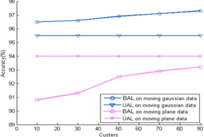
Fig. 11. Effect of the number of clusters on the performance.
1) Effect of the Data Distribution: In order to capture the data distribution’s effect, we evaluate BAL’s performance on Gaussian (mixture drift) and uniformly (gradual drift) distributed data with respect to the number of clusters. Here, the budget is fixed to 0.05. Fig. 11 shows the performance on both data sets. Incorporating density-based criterion clearly improves the performance on the Gaussian data.
For the case of uniformly distributed data, density-based criterion yields lower performance than UAL. However, for both data sets, the accuracy improves as the number of clusters increases (see Table III). The uniform distribution is the most extreme break for the Gaussian assumption. However, BAL has good performance compared with UAL when remote drift occurs. Fig. 12 shows that BAL can adapt faster to abrupt remote drift. Based on these experiments, BAL shows great potential in maintaining higher classification over time.
TABLE III
EFFECT OF THENUMBER OFCLUSTERS ONBAL ACCURACY: CASE OFPLANE ANDGAUSSIANDATA
TABLE IV
ACCURACY OFBAL COMPAREDWITHRANDOMSAMPLING USINGDIFFERENTBUDGETVALUES(SYNTHETICDATA)
2) Effect of the Budget: Table IV illustrates the average accuracy of BAL compared with random sampling (baseline) on the three types of drift (gradual, abrupt, and mixture) using different budgets. The values with star indicate that the additional budget is not used. To cope with abrupt drift, BAL does not need big budget to show high accuracy. However, budget has more impact on the accuracy in the case of gradual drift. Mixture drift requires less budgets than the gradual drift and more budget than abrupt drift.
C. Simulation on Real-World Data
Two real-world benchmark data sets: Electricity and Air-lines are used to evaluate BAL in more challenging set-tings. Their characteristics are shown in Table V. Electricity
Fig. 12. Sensitivity to remote drift. TABLE V
CHARACTERISTICS OF THEREAL-WORLDDATASETS
data [36] is a popular benchmark used in evaluating classifi-cation in the context of data streams. The task is to predict the rise or fall of electricity prices (demand) in New South Wales (Australia), given recent consumption and prices in the same and neighboring regions. The Airlines data set was collected by the USA flight control [37]. The task is to predict whether a flight will be delayed given the scheduled departure time.
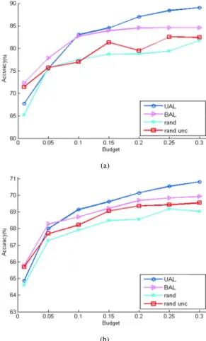
To illustrate the performance of BAL compared with the state-of-the-art AL algorithms over data streams, two meth-ods are considered: Random (baseline method) and Variable Randomized Uncertainty proposed in [7]. Unlike BAL, the method described in [7] depends on the internal classification algorithm (learning engine). Here, we use the Naive Bayes classifier as a learning engine as in [7]. Only the first 10% of the data sequence for both data sets are used. The parameters of GGMM are empirically set to the values shown in Table II. In this experiment, the algorithms are evaluated using dif-ferent budgets in [0.01;0.3]. The final accuracy results are reported in Fig. 13, which show that UAL outperforms the rest of the competitors for high budget, while BAL works better for low budget (10 % for Electricity and 7% for Airlines).˜ D. Discussion
While the performance of UAL and BAL is far better than the competitors, the application of the uncertainty criterion solely becomes more valuable as more data are queried (high
Fig. 13. Results related to the real-world data sets. (a) Electricity data. (b) Airlines data.
budget). This finding was already shown in previous studies in the context of batch-based learning [13]. In the case of drifting data where the boundary between classes is very dynamic like with Electricity and Airlines data, the samples close to the boundary are more interesting, since they drive the change in the distribution. Increasing the number of queries (i.e., high budget) will definitely enhance the accuracy irrespective of the data density; hence, UAL performs better than BAL when the budget is high. This is in contrast to the case of drifting synthetic data where BAL performs better and has a recovery speed faster than UAL.
Zliobaite et al. [7] claimed that the Electricity data have more aggressive drift than the Airlines data, which may explain the difference between the accuracy improvement associated with density-based criterion over the two data sets. BAL accuracy is better than UAL over the Airlines data only for budget less than 0.07, while it is up to 0.1 in the case of Electricity data. However, clearly the proposed UAL and BAL could be dynamically combined yielding one model that gives better results under any kind of drift over the whole budget line where BAL selects data for low budget, while UAL takes control for high budget.
VII. CONCLUSION ANDFUTUREWORK
We proposed an AL algorithm for data streams to deal with changes of the data distribution. BAL labels the samples with high uncertainty and representativeness in a completely
online scenario. It also tackles the sampling bias of AL with potentially adversarial concept drift. Experimental results on real-world data showed the limitation of the proposed approach when the budget is high or the drift occurrence is rare and smooth. However, the main goal of reducing the labeling cost in the presence of concept drift, while maintaining good accu-racy, has been achieved. Experimental results on synthetic data showed that as the data distribution becomes more uniform, more clusters are needed, and the time complexity increases. However, the maximum number of clusters is fixed, and we can have a lower bound on the time complexity. Therefore, based on the data stream velocity, we can decide the maximum number of clusters allowed. Finally, many experiments have been carried out in order to come up with an approximation of local optimal values for GGMM’s parameters. This is the main drawback of the proposed method and an improvement will be done in the next step of this research by reducing the effect of parameter settings.
In the future, we will improve BAL to accommodate data with any distribution by using nonparametric models that require less number of parameters and possibly unknown number of classes. We will also provide dynamic combination between BAL and UAL as stated Section VI-D. We also aim at addressing a number of outstanding questions associated with online AL such as follows.
1) Are the labels provided by the oracle always accurate? How long does it take the oracle to provide the label? 2) What are the variables that might affect the budget? 3) How can prior knowledge about drift be exploited? These are all interesting open issues worth exploring in the context of data stream classification.
REFERENCES
[1] A. Bouchachia and C. Vanaret, “GT2FC: An online growing interval type-2 self-learning fuzzy classifier,” IEEE Trans. Fuzzy Syst., vol. 22, no. 4, pp. 999–1018, Aug. 2014.
[2] A. Bouchachia, “Incremental learning with multi-level adaptation,”
Neurocomputing, vol. 74, no. 11, pp. 1785–1799, May 2011.
[3] B. Settles, “Active learning literature survey,” Univ. Wisconsin, Madison, vol. 52, pp. 55–66, Jan. 2010.
[4] K. Lang and E. Baum, “Query learning can work poorly when a human oracle is used,” in Proc. IEEE Int. Joint Conf. Neural Netw., 1992, pp. 335–340.
[5] S. Tong and E. Chang, “Support vector machine active learning for image retrieval,” in Proc. ACM MULTIMEDIA, 2001, pp. 107–118. [6] B. Settles and M. Craven, “An analysis of active learning strategies
for sequence labeling tasks,” in Proc. Conf. Empirical Methods Natural
Lang. Process., 2008, pp. 1070–1079.
[7] I. Zliobaite, A. Bifet, B. Pfahringer, and G. Holmes, “Active learning with drifting streaming data,” IEEE Trans. Neural Netw. Learn. Syst., vol. 25, no. 1, pp. 27–39, Jan. 2014.
[8] D. Cohn, L. Atlas, and R. Ladner, “Improving generalization with active learning,” Mach. Learn., vol. 15, no. 2, pp. 201–221, May 1994. [9] S. Dasgupta, “Two faces of active learning,” Theoretical Comput. Sci.,
vol. 412, no. 19, pp. 1767–1781, Apr. 2011.
[10] A. Bouchachia, “On the scarcity of labeled data,” in Proc. Int. Conf.
Comput. Intell. Modelling, Control Autom. Int. Conf. Intell. Agents, Web Technol. Int. Commerce, Nov. 2005, pp. 402–407.
[11] Z. Xu, K. Yu, V. Tresp, X. Xu, and J. Wang, Representative
Sampling for Text Classification Using Support Vector Machines.
New York, NY, USA: Springer, 2003.
[12] H. T. Nguyen and A. Smeulders, “Active learning using pre-clustering,” in Proc. Twenty-First Int. Conf. Mach. Learn., 2004, p. 79.
[13] P. Donmez, J. G. Carbonell, and P. N. Bennett, “Dual strategy active learning,” in Proc. Europ. Conf. Mach. Learn., 2007, pp. 116–127.
[14] S. Tong and D. Koller, “Support vector machine active learning with applications to text classification,” J. Mach. Learn. Res., vol. 2, pp. 45–66, Mar. 2001.
[15] D. D. Lewis and W. A. Gale, “A sequential algorithm for training text classifiers,” in Proc. 17th Annu. Int. ACM SIGIR Conf. Res. Develop.
Inf. Retr., 1994, pp. 3–12.
[16] A. Beygelzimer, S. Dasgupta, and J. Langford, “Importance weighted active learning,” in Proc. 26th Annu. Int. Conf. Mach. Learn., New York, NY, USA, 2009, pp. 49–56. [Online]. Available: http://doi.acm.org/10.1145/1553374.1553381
[17] J. Attenberg and F. Provost, “Online active inference and learning,” in
Proc. 17th ACM SIGKDD Int. Conf. Knowl. Discovery Data Mining,
2011, pp. 186–194.
[18] D. Sculley, “Online active learning methods for fast label-efficient spam filtering,” in Proc. 4th Conf Email Anti-Spam, Mountain View, CA, USA, 2007, pp. 1–4.
[19] D. H. Widyantoro and J. Yen, “Relevant data expansion for learning concept drift from sparsely labeled data,” IEEE Trans. Knowl. Data
Eng., vol. 17, no. 3, pp. 401–412, Mar. 2005.
[20] M. M. Masud et al., “Facing the reality of data stream classification: Coping with scarcity of labeled data,” Knowl. Inf. Syst., vol. 33, no. 1, pp. 213–244, Oct. 2012.
[21] P. Lindstrom, S. J. Delany, and B. M. Namee, “Handling concept drift in text data stream constrained by high labelling cost,” in Proc. 23rd
Int. Florida Artif. Intell. Res. Soc. Conf., 2010pp. 19–21.
[22] J. Read, A. Bifet, B. Pfahringer, and G. Holmes, “Batch-incremental versus instance-incremental learning in dynamic and evolving data,” in
Proc. 11th Adv. Intell. Data Anal., 2012, pp. 313–323.
[23] D. A. Cohn, Z. Ghahramani, and M. I. Jordan. (Mar. 1996). “Active learning with statistical models.” [Online]. Avaliable: https://arxiv.org/abs/cs/9603104
[24] J. Gama, I. Žliobait˙e, A. Bifet, M. Pechenizkiy, and A. Bouchachia, “A survey on concept drift adaptation,” in Proc. ACM Comput. Surv., vol. 46, no. 4, 2014, Art. no. 44.
[25] C. M. Bishop, Neural networks for pattern recognition. Oxford, U.K.: Clarendon Press, 1995.
[26] G. E. Box and G. C. Tiao, Bayesian Inference in Statistical Analysis, vol. 40. Hoboken, NJ, USA: Wiley, 2011,
[27] W. D. Penny and S. J. Roberts, “Dynamic logistic regression,” in Proc.
Int. Joint Conf. Neural Netw., vol. 3. Jul. 1999, pp. 1562–1567.
[28] J. D. Banfield and A. E. Raftery, “Model-based Gaussian and non-Gaussian clustering,” Biometrics, vol. 49, no. 3, pp. 803–821, Sep. 1993. [29] C. Stauffer and W. E. L. Grimson, “Learning patterns of activity using real-time tracking,” IEEE Trans. Pattern Anal. Mach. Intell., vol. 22, no. 8, pp. 747–757, Aug. 2000.
[30] K. P. Murphy, Machine learning: A Probabilistic Perspective.
Cambridge, MA, USA: MIT press, 2012.
[31] D. J. Spiegelhalter and S. L. Lauritzen, “Sequential updating of condi-tional probabilities on directed graphical structures,” Networks, vol. 20, no. 5, pp. 579–605, Aug. 1990.
[32] J. Freitas, M. Niranjan, and A. Gee, “Hierarchical Bayesian models for regularization in sequential learning,” Neural Comput., vol. 12, no. 4, pp. 933–953, Apr. 2000.
[33] J. Gama, R. Sebastião, and P. P. Rodrigues, “On evaluating stream learn-ing algorithms,” Mach. Learn., vol. 90, no. 3, pp. 317–346, Mar. 2013. [34] J. S. Liu, Monte Carlo Strategies in Scientific Computing.
New York, NY, USA: Springer, 2001.
[35] A. M. Narasimhamurthy and L. I. Kuncheva, “A framework for gener-ating data to simulate changing environments,” Artif. Intell. Appl. 2007, pp. 415–420.
[36] M. B. Harries, C. Sammut, and K. Horn, “Extracting hidden context,”
Mach. Learn., vol. 32, no. 2, pp. 101–126, Aug. 1998.
[37] E. Ikonomovska, J. Gama, and S. Džeroski, “Learning model trees from evolving data streams,” Data Mining Knowl. Discovery, vol. 23, no. 1, pp. 128–168, Jul. 2011.
[38] H. Toubakh and M. Sayed-Mouchaweh, “Hybrid dynamic classifier for drift-like fault diagnosis in a class of hybrid dynamic systems: Application to wind turbine converters,” Neurocomputing, vol. 171, pp. 1496–1516, Jan. 2015.