Multitarget Tracking with
Interacting Population-based MCMC-PF
Mélanie Bocquel, Hans Driessen
Thales Nederland B.V. - Sens TBU Radar Engineering, Hengelo, Nederland
Email: {Melanie.Bocquel, Hans.Driessen} @nl.thalesgroup.com
Arun Bagchi
University of Twente - Department of Applied Mathematics Enschede, Nederland
Email: [email protected]
Abstract—In this paper we address the problem of tracking multiple targets based on raw measurements by means of Particle filtering. This strategy leads to a high computational complexity as the number of targets increases, so that an efficient implementation of the tracker is necessary.
We propose a new multitarget Particle Filter (PF) that solves such challenging problem. We call our filter Interact-ing Population-based MCMC-PF (IP-MCMC-PF) since our ap-proach is based on parallel usage of multiple population-based Metropolis-Hastings (M-H) samplers. Furthermore, to improve the chains mixing properties, we exploit genetic alike moves performing interaction between the Markov Chain Monte Carlo (MCMC) chains.
Simulation analyses verify a dramatic reduction in terms of computational time for a given track accuracy, and an increased robustness w.r.t. conventional MCMC based PF.
I. INTRODUCTION
Multitarget tracking is a well-known problem which consists of sequentially estimating the states of several targets from noisy data. It arises in many applications, e.g. radar based tracking of aircraft. Bayesian methods provide a rigorous general framework for dynamic state estimation problems. The Bayesian recursions update the posterior probability density function (pdf) of the state based on all available information, including the set of received measurements. The application of the Bayesian sequential estimation framework to multitarget tracking problems is plagued by two difficulties. First, the state and observation models are often non-linear and non-Gaussian, so that no closed-form analytic expression can be obtained for the tracking recursions. The second difficulty is due to the fact that in most practical tracking applications the sensors yield unlabeled measurements of the targets. This leads to a challenging data association problem.
The multitarget tracking problem has been traditionally addressed with techniques such as multiple hypothesis tracking (MHT) and joint probabilistic data association (JPDA), which require plot measurements (detection) and a measurement-to-track association procedure [1]. Solutions using a Particle Filter (PF) have been proposed in the past ten years [2]–[4]. These so-called Track-Before-Detect (TBD) approaches define a model for the raw measurements in terms of a multi-target state hypothesis, thus avoiding an explicit data association step. Furthermore, as opposed to the conventional thresholded measurement procedure, these strategies allow the tracker to perform well in the low Signal-to-Noise Ratio (SNR) regime.
Particle filtering is a Sequential Monte Carlo (SMC) simulation-based method of approximately solving the Bayes prediction and update equations recursively using a stochastic samples (particles) cloud [5]. The Sampling Importance Re-sampling (SIR) Multitarget PF, that recursively estimates the joint multitarget probability density (JMPD), has demonstrated its ability to successfully perform nonlinear and non-Gaussian tracking and to enable more accurate modeling of the target correlations. While the SIR PF is fairly easy to implement and tune, its main drawbacks are the computational complexity which increases rapidly with the state dimensions and the loss of diversity among the particles due to resampling. To mitigate the former problem an adaptive sampling strategy, called the Adaptive Proposal (AP) method [3], has been suggested. This strategy proposes to construct particle proposals at the partition level, incorporating the measurements so as to bias the pro-posal towards the optimal importance density. The AP method automatically factors the JMPD when targets are behaving independently [6], while attempt to handle the permutation symmetry and correlations that arise when targets are coupled [3]. The latter problem can effectively be addressed by using Particle MCMC (PMCMC) methods [7], [8], e.g. the Particle Marginal Metropolis-Hastings (PMMH) algorithm.
In recent years there has been an increasing interest towards Markov Chain Monte Carlo (MCMC) methods to simulate complex, nonstandard multivariate distributions. There are two basic MCMC techniques: the Gibbs sampler [9], [10], and the Metropolis-Hastings (M-H) [11], [12] algorithm. The former method is based on sampling from the collection of full conditional distributions, while the latter approach is a generalization that can be used when the full conditionals cannot be written in a closed form.
Recently, the research done on Markov chains and Hidden Markov Models has led the definition of the M-H algorithm through the notion of reversibility [13], and allowed for the derivation of convergence results for Sequential MCMC methods, e.g. the PMCMC. Although these methods are very reliable, the computational expense of PMCMC algorithms for complex models remains a limiting factor. Furthermore, the mixing of the resulting MCMC kernels can be quite sensitive, both to the number of particles and the measurement space dimension.
In this paper we focus on issues arising in the imple-mentation of multitarget Bayesian filtering. Thus, we pro-pose an alternative algorithm, which fully exploits the speed and the parallelism of modern computing architectures and resources. We introduce a new M-H based PF in which several MCMC chains will be running in parallel, this way generatingpopulation-basedsamples to approximate the target distribution. Furthermore, to improve themixing propertiesof the resulting MCMC kernel, the diversity of each population is increased by means of an interaction procedure[14]. Note that we will assume throughout this paper that the number of targetsM is known and constant over time.
The paper is organized as follows: in section II we review the Bayesian Filtering problem; section III briefly reviews the basics of particle filtering and MCMC methods for sampling. Section IV reports the main part of our work. Here we introduce our new algorithm, which we called Interacting Population-based MCMC-PF (IP-MCMC-PF), discuss the im-provements attainable by using a fully parallelizable PF, and give theoretical justifications for our approach. In section V the system dynamics and measurement model are introduced for the specific TBD surveillance application. Section VI collects our simulations results. Finally, we report our conclusions and direction for future research in section VII.
II. BAYESIANFILTERINGPROBLEM
In this section, we briefly describe the Bayesian Filtering problem. Let us consider the following dynamical system:
xk+1 =fk(xk,vk), (1) zk =hk(xk) +wk, (2) where xk ∈ Rnx denotes the state vector, zk ∈
Rnz the
system measurement, vk ∼ pvk(v) the process noise, and
wk∼pwk(w)the measurement noise.
Furthermore, let Zk , {z1, . . . ,zk} be the sequence of
measurements collected up to time k. The measurement zk is assumed to be independent from the past states, i.e.,
p(zk|zk−1, . . . ,z1,xk,xk−1, . . . ,x0) =p(zk|xk), (3)
wherep(zk|xk)denotes thelikelihood function.
Given a realization of Zk, Bayesian filtering boils down to finding an approximation of the posterior pdf p(xk|Zk). In particular, the marginal filtering distribution p(xk|Zk) is obtained at time kby means of a two-step recursion: (1) the Prediction Step, which is solved using the Chapman-Kolmogorov equation, i.e.,
p(xk|Zk−1) =
Z
p(xk|xk−1)p(xk−1|Zk−1)dxk−1 (4)
where, p(xk|Zk−1)is the predictive density at timek;
(2) the Update Step, which is solved usingBayes theorem, i.e.,
p(xk|Zk) =p(zk|xk)p(xk|Zk−1) p(zk|Zk−1)
(5)
where p(zk|Zk−1) is the Bayes normalization constant
(evi-dence). Thus, the filtering pdf is completely specified given
some prior p(x0), a transition kernelp(xk|xk−1)and a
like-lihoodp(zk|xk).
Given the a posteriori pdfp(xk|Zk), some averaged statis-tics of interest can be calculated, e.g. the mean-squared error (MSE), i.e.,
E[kxk−xˆkk2|Zk] = Z
kxk−xˆkk2p(xk|Zk)dxk, which can be used to derive the minimum variance estimator,
ˆ
xM Vk , Z
xk p(xk|Zk)dxk. (6)
III. FUNDAMENTALS
In this section we recall the basics of Markov Chain Monte Carlo, Particle Filtering and Particle MCMC methods, necessary for clarifying the strengths of our method. In fact, in section IV we propose an approach for state estimation that combines the differing pros of both MCMC and PF based signal processing. Specifically, subsection III-A is dedicated to MCMC methods; subsection III-B reviews Particle Filtering techniques; while subsection III-C is used to discuss related work on Particle MCMC methods.
A. Basic of Markov Chain Monte Carlo process
Let X ⊆ RM be a compact set and suppose that π(x) is
a probability distribution on such a high-dimensional space X. Denote by B(X) the Borel σ-field and by (X,B(X))
the associated measure space. Then, thanks to Markov chains theory and Monte Carlo sampling, the following holds:
A Markov Chain Monte Carlo method for the simulation of the distribution π is any method which generates an ergodic Markov chain{x(ki)}i≥1 onX, according to a kernelK(., .)
defined on (X × B(X)), withπas stationary distribution. Let us recall two basic concepts:
1) πis thestationary distributionof the Markov chain, i.e., for allA∈ B(X),
π(A) =
Z
X
K(x, A)π(x)dx. (7)
2) The Markov chain is ergodic, i.e. for any integrable functionq:X →R lim N→∞ 1 N N X i=1 q(x(ki))→Eπ(q) = Z X q(x)π(x)dx (8)
with probability1,∀x(0)k ∈ X, whereN is the number of iterations of the MCMC algorithm.
The Metropolis-Hastings (M-H) algorithm [15] is a well known procedure based on a Markovian process which ful-fills the requirement of ergodicity [16]. The M-H algorithm employs a conditional density q, also known as proposal distribution, to generate a Markov chain with an invariant distribution π. At each MCMC iteration i, a move x0 ∼
q(x0|x(i−1)) is proposed and accepted with a probability
Notice that the initial burn-in samples are strongly influ-enced by the initial configuration, so discarding them increases the speed of convergence towards the stationary distribution.
Let us now consider a multitarget setting where xk = [xk,1, ...,xk,M]is the multitarget base state vector, with xk,j
being the state vector of the jth target at timek. Within the Bayesian estimation framework, the target distribution π is chosen as the approximate posterior distribution,
π(x(ki−1)) =p(xk(i−1)|Zk)∝p(x
(i−1)
k )p(Zk|x
(i−1)
k ). (9) The acceptance ratio is then given by:
α= p(x 0)p(Zk|x0)q(x(i−1) k |X0) p(x(ki−1))p(Zk|xk(i−1))q(x0|x(i−1) k ) . (10)
A suitably designed proposal distribution is fundamental to guarantee a well mixing Markov chain. The efficiency of the M-H algorithm is strongly influenced by such choice. In particular, this problem becomes central when dealing with high dimensional and interdependent state vectors.
Such distributions should both be easy to sample from and allow the Markov chain to explore all the high density regions of X under π freely. However, the design of such efficient proposal distributions might be problematic. Instead, local strategies, focusing on some of the subcomponents ofπ, e.g. propose to move one target at each time, x0j∼q(x0j|x(k,ji−1)) are often used, to break up the original sampling problem into simpler ones. Nevertheless, these can be prone to poor performance, as local strategies inevitably ignore some of the global features ofπ.
In summary, Markov Chain Monte Carlo (MCMC) methods are convenient and flexible, but they require to meet the following conditions :
• A sufficiently long burn-in time to allow convergence.
• Enough simulation draws for a suitably accurate inference for estimating the distribution π.
Note however that the convergence of MCMC algorithms strongly depends on whether the model actually fits the data and, in particular, the quality of the proposal distribution. Therefore convergence problems are often related to modeling issues.
B. Basic of Particle Filtering
A Particle Filter is known for its ability to tackle nonlinear and non-Gaussian problems. The detailed PF algorithm, as introduced in [17], is described below. At time step k−1, the posterior pdf p(xk−1|Zk−1) is approximated by a set of
particles{x(ki−1) }Np
i=1with associated weights{w (i)
k−1}
Np
i=1. Each
particlex(ki−1) is passed through the system dynamics eq.(1)to obtain {ˆx(ki)}Np
i=1, the predicted particles at time stepk. Once
the observation data zk is received, the importance weight of each predicted particle can be evaluated according to the weight equation reduces to:
˜
w(ki)=p(zk|ˆx(ki))
Then, after normalization of the weights, the a posteriori density p(xk|Zk) at time stepk can be approximated by the empirical distribution as : ˆ p(xk|Zk) := Np X i=1 w(ki) δˆx(i) k (xk), (11) where δˆx(i) k
(.) denotes the delta-Dirac mass located at xˆ(ki). See [18] for a proof and [19] for more detail and an overview of convergence results.
Finally, a resampling step is used to prevent the variance of the particle weights to increase over time. Although the resampling step reduces the effects of the degeneracy problem, it introduces other practical problems. First, it limitsparallel processing since all particles have to be combined. Second, by resampling the posterior distribution, the heavily weighted particles are statistically selected several times. This leads to a loss of diversity among the particles, thesample impoverish-mentproblem. In the extreme case, all the particles collapse to the same location. The sample impoverishment leads to failure in tracking since less diverse particles are used to represent the uncertain dynamics of the moving object. Both problems can effectively be handled by using a MCMC method implemented by e.g. the M-H algorithm.
C. Particle Markov chain Monte Carlo (PMCMC)
Several algorithms combining MCMC and SMC approaches have already been proposed in the literature [7], [20], [21]. Recently, Andrieu, Doucet and Holenstein [8] introduced a general framework, known as Particle MCMC (PMCMC), which uses a PF to construct proposal kernels for an MCMC sampler. PMCMC algorithms can be thought of as natural approximations to standard and idealized MCMC algorithms which cannot be implemented in practice. This framework provides three powerful methods for joint Bayesian state and parameter inference for nonlinear, non-Gaussian state-space models. These methods are referred to as Particle Independent Hastings (PIMH), Particle Marginal Metropolis-Hastings (PMMH) and Particle Gibbs (PG). In particular, the PMMH algorithm aims an exact approximation of aMarginal Metropolis-Hastings (MMH) update. The implementation of the PMMH scheme requires an SMC approximation targeting
p(x0:k|Zk, θ)and the filter estimate of the marginal likelihood
p(Zk|θ)withθ∈Θsome static parameter. Full details of the PMMH scheme including a proof establishing that the method leaves the full joint posterior density p(θ,x0:k|Zk) invariant can be found in [8].
However, note that to obtain reasonable mixing of the resulting MCMC kernels, it was reported in [8] that a fairly high number of particles was required in the SMC scheme. Since every iteration of the PMMH scheme requires a run of a PF, a lot of computational resources are needed. In fact, if a PF algorithm usingNpparticles is applied at each iteration, then the computational complexity of the PMCMC algorithm isO(Np M N), whereN is the number of MCMC iterations andM =dim(xk). In the following section we will propose
an alternative algorithm, which is much more robust to a low number of particles, and well suited to deal with tracking problems.
IV. INTERACTINGPOPULATION-BASEDMCMC-PF In this section, we will present the Interacting Population-based MCMC-PF (IP-MCMC-PF) algorithm. We will give theoretical justifications for our approach and discuss the improvements attainable by using a fully parallelizable PF.
A. Justifications behind the IP-MCMC-PF algorithm There are two basic ideas behind the proposed algorithm : (1) Reliable statistical inferences for the target distribution are required. For this purpose we run multiple MCMC sam-pling chains each starting from different seeds, in parallel. A single possibly time varying transition kernel is used for all parallel chains. The only difference is the region of the space explored by each chain. The simulations from the chains are spread across various high probability regions of the target distribution. After a sufficiently long burn-in period, each chain reaches the stationary distribution. This means that, once enough stationary simulations have been drawn, mixing all sets of draws provides a good estimate of the target distribution.
(2) Rapid mixingwithin each MCMC chain is required. We want to speed upthe MCMC convergence ratefor minimizing the burn-inperiod. For that the history from all the chains is used to adapt the kernel and therefore to guide any particular population member in the exploration of the state space toward regions of higher probability. Thus more global moves (than independent MCMC chains) can be constructed. This ensures the least correlation among a single particle’s history states resulting in faster mixing within each MCMC chain.
Furthermore the proposed implementation resorts to within-chain analysis to monitor stationarity and between/within chains comparisons to monitor mixing. Combined, stationarity and mixing lead to the convergence of the set of MCMC chains.
B. IP-MCMC-PF algorithm and challenges of implementation In the proposed IP-MCMC-PF algorithm, the posterior distribution over target states at timek−1is represented by a set ofNpparticles{x
(i)
k−1}
Np
i=1. Each particle contains the joint
state ofM partitions corresponding to the different targets. We refer to x(ki−1) ,j as the states of thejthpartition of the particle
i at time stepk−1. The particle state vector is given by :
xk(i−1) =hxk(i−1) ,1, . . . ,x(ki−1) ,Mi.
Let us denote NMCMC the optimal number of MCMC chains
that can operate in parallel. The parameter NMCMC depends on
firstly, the experiment setup (targets in track and modelling complexity) and secondly, the system specification (parallel processing potential, memory resources). At each time step
k, NMCMC particles are randomly selected from {x (i)
k−1}
Np
i=1.
These particles are then propagated based on the dynamic model eq.(1)to obtain the predicted random subset of particles
{ˆy(0)s }Ns=1MCMC. The predicted particles are then chosen as the starting points in the MCMC sampling procedure.
The MCMC sampling procedure consists to run NMCMC
M-H samplers in parallel. Each sampler s is initiated with the configuration {ˆy(0)s ;`
(0)
s } and is used to generate a set of
N samples from p(xk|Zk). At each MCMC iteration nM-H,
a partitionj of a random particleipicked out of {x(ki−1) }Np
i=1
is randomly selected. Given this partition x(ki−1) ,j, a partition move y0 is proposed. This move seeks to update the
sin-gle partition x(ki−1) ,j via a Markov kernel that describes the state dynamic eq.(1). This move, also known as Mutation (Genetic Algorithm see [22]), allows for local exploration of the state space, as well as ensuring the required irreducibility of the Markov chain. Then, given {ˆys(nM-H−1);`
(nM-H−1)
s } the previous configuration, a new configuration {˜ys(nM-H);`˜(snM-H)} is obtained by replacing the partition j by y0 and updating the joint log-likelihood. This new configuration is proposed and accepted as the next realization from the chain s with a probability
0<min1, α(ˆys(nM-H−1),˜y(snM-H))<1.
The acceptance ratio only depends on the likelihoods and is given by : α(ˆy(snM-H−1),˜y(nM-H) s ) = ˜ `(snM-H) `(snM-H−1) . (12)
Note that such M-H move can be seen as an Exchange move (Genetic Algorithm see [22]). It can be proven that information exchange between MCMC chains targeting close distributions does not effect convergence properties [16]. Furthermore, in the proposed procedure, the MCMC sampling chains swap information within the M-H samplers without effecting the parallel processing. At the end of the procedure, the ini-tial burn-in simulations, which are strongly influenced by starting values, are discarded, while the remaining samples {ˆy(nM-H)
s }BnM-H+N=B+1 are stored as new particles to summarize
the target distribution at time stepk.
In the proposed algorithm, a validation test is performed to check the convergence on the basis of Gelman and Rubin [23] diagnostic. The potential scale reduction factor (PSRF)Rˆ can be used for such test. In fact,R, defined asˆ
ˆ
R=
q
¯
C/W¯ , (13)
withC¯ the empirical variance from all chains combined and
¯
W, the mean of the empirical within-chain variances, provides an ANOVA-like comparison of the within-chain and between-chain variances, i.e.
• Rˆ = 1, then the MCMC chains have converged within
the burn-in period.
• Rˆ >1, then all the MCMC chains have not fully mixed
and that further simulation might increase the precision of inferences.
If the PSRF is close to 1, we can conclude that each of the
NMCMC sets of N simulated observations is close to the target
distribution. In the proposed algorithm the parallel chains are considered well-mixed whenRˆ is less or equal than1.1 (the PSRF is estimated with uncertainty because our MCMC chain lengths are finite).
Once the set of chains have reached approximate conver-gence, the MCMC sampling chains outputs, i.e. the NMCMC
sets of simulations, mixed all together give the new set of particles{x(ki)}Np
i=1which approximates the target distribution
p(xk|Zk).
The proposed IP-MCMC-PF algorithm is summarized in Algorithm 1. Then, a pseudo-code description of the MCMC sampling procedure is given by Algorithm 2.
Algorithm 1: IP-MCMC-PF algorithm input : {x(ki−1) }Np
i=1 and a new measurement,zk.
output: {x(ki)}Np
i=1.
1 - Initialisation starting points:
Select a random subset{y(0)s }Ns=1MCMC ⊂ {x (i)
k−1}
Np
i=1
while s←1 toNMCMC do
Predict a new particle state at time k: while j←1 toM do ˆ ys,j(0)=fk(y (0) s,j) +v (i) k−1,j. end
Compute the associated joint log-likelihood:
`(0)s = logp(Zk|ˆy
(0)
s ). end
Store the new states in a cache {ˆys(0);`(0)s }Ns=1MCMC.
2 - MCMC sampling procedure:
Run NMCMC Metropolis-Hastings samplers in parallel
(Algorithm 2) to obtain {y(si)} wherei= 1, . . . , N and
s= 1, . . . , NMCMC.
3 - Checking convergence: ComputeR: (eq. 13).ˆ if Rˆ ≥1.1 then
Run the chains out longer to improve convergence to the stationary distribution.
else
Mix all theNMCMC set of simulations together to
obtain {x(ki)}Np
i=1.
end
V. SYSTEMSETUP ANDTBD PROBLEMFORMULATION
In this section, we will describe the system dynamic model and the measurement model.
Let us denote by xk,j the vector describing the state of the
jth target(j∈ {1, M})at time stepk written as:
xk,j = [sk,j, ρk,j]T (14) where, sk,j represents the position and velocity of the jth target in Cartesian coordinates and ρk,j is the unknown
Algorithm 2: MCMC sampling procedure
input : {ˆys(0);`s(0)}Ns=1MCMC initial configurations,Np required number of samples,B number of burn-in samples.
output: {y(si)}wheres= 1, . . . , NMCMC andi= 1, . . . , N
withN :=Np/NMCMC.
whiles←1 to NMCMC do fornM-H←1 toB+N do
1 - Proposal of move:
Randomly select a partitionx(ki−1) ,j out of {x(ki−1) }Np i=1; Givenx(ki−1) ,j, drawy0=fk(x (i) k−1,j) +v (i) k−1,j; Proposey˜(nM-H) s byy0→ˆy (nM-H−1) s ;
Compute the joint log-likelihood: ˜
`(snM-H)= logp(Zk|˜y
(nM-H)
s ).
2 - M-H acceptance:
Sampleu∼ U[0,1],U[0,1] a uniform distribution in
[0,1];
Compute the M-H acceptance probability
α(yˆs(nM-H−1),y˜ (nM-H) s ): (eq. 12). ifu≤min (1, α)then Accept move: {ˆy(nM-H) s ;` (nM-H) s }={˜y (nM-H) s ;˜` (nM-H) s }, else Reject move: {ˆys(nM-H);`(snM-H)}={ˆy(snM-H−1);`(snM-H−1)}. end end
Discard B initial burn-in samples, store the remaining samplesˆy(sB+1:B+N)→ {y
(i)
s }Ni=1.
end
modulus of the target complex amplitude. The state vectors
(xk,j)j∈{1,M} can be concatenated into the multitarget state vectorxk.
A. Dynamic model
To model the dynamics of the targets we adopt a nearly con-stant velocity model to describe object position and velocity in a Cartesian frame, see e.g. [4], and a random walk model for object amplitude ρk,j. The model uncertainty is handled by the process noisevk,j, which is assumed to be standard white Gaussian noise with covariance G. Under these assumptions, the corresponding state-space model, forxk,j, the state vector associated to thejthtarget, is given by:
xk+1,j =Fxk,j+vk,j, (15) whereF represents a transition matrix with a constant sam-pling timeT such as:
F = diag(F1, F1,1), where, F1 = 1 T 0 1 . (16)
andG, the covariance process noise, is given by: G = diag(axG1, ayG1, aρT), where, G1 = " T3 3 T2 2 T2 2 T # , (17)
where ax =ay andaρ denote the level of process noise in object motion and amplitude, respectively. This model cor-rectly approximates small accelerations in the object motion and fluctuations in the object amplitude.
B. Measurement model
At discrete instants k, the radar system positioned at the Cartesian origin collects a noisy signal. Each measurement zk consists ofNr×Nd×Nb reflected power measurements zlmn
k , whereNr,Nd andNbare the number of range, doppler and bearing cells. The power measurement per range-doppler-bearing cell is defined by :
zlmnk =|zlmnρ,k |2, k∈N. (18)
where zlmnρ,k is the complex envelope data of the target de-scribed by the following nonlinear equation, see [4]:
zlmnρ,k = M X j=1 ρk,jeiϕkhlmn(sk,j) +wklmn, ϕk∈(0,2π) (19) wherehlmn(sk,j)is the reflection form of thejthtarget, that for every range-doppler-bearing cell is defined by:
hlmn(xk,j) :=e− (rl−rk,j)2 2R − (dm−dk,j)2 2D − (bn−bk,j)2 2B , (20) l= 1, . . . , Nr, m= 1, . . . , Nd, n= 1, . . . , Nb andk∈N
where the relationship between the measurement space and the target space can be established as:
r=px2+y2, d=(x vx+y vy) p x2+y2 andb= arctan y x . (21)
R,DandBare related to the resolutions in range, doppler and bearing. wlmn
k are independent samples of a complex white Gaussian noise with variance2σ2
w,(i.e.the real and imaginary components are assumed to be independent, zero-mean white Gaussian with the same variance σ2w).
C. TBD Problem Formulation
Consider the system represented by the equations (15), (18) and (19). Assume that the set of measurements collected up to the current time is denoted by Zk = {z1, . . . ,zk}. The
filtering problem can be formulated as finding the a posteriori distribution of the joint state xk for all possible numbers of targets conditioned on all past measurementsZk.
VI. SIMULATION SETUP ANDRESULTS
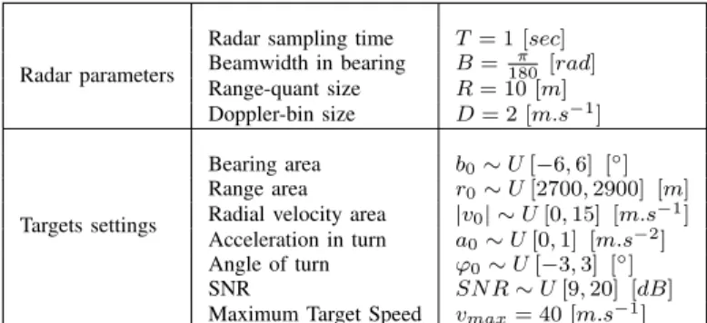
In this section the multitarget TBD filtering problem has been recursively solved by running the IP-MCMC-PF on the power measurements. We investigate through simulations the improvements provided by interacting population-based simu-lation over standard SMC and MCMC methods. Simusimu-lations are performed with a typical ground radar scenario (one or several targets move in the x-y plane at unknown constant velocity). The radar parameters and the targets settings used in simulation are reported in Table I.
TABLE I
PARAMETERS USED IN SIMULATION
Radar parameters
Radar sampling time T = 1 [sec]
Beamwidth in bearing B=180π [rad]
Range-quant size R= 10 [m]
Doppler-bin size D= 2 [m.s−1]
Targets settings
Bearing area b0∼U[−6,6] [◦] Range area r0∼U[2700,2900] [m] Radial velocity area |v0| ∼U[0,15] [m.s−1] Acceleration in turn a0∼U[0,1] [m.s−2] Angle of turn ϕ0∼U[−3,3] [◦] SNR SN R∼U[9,20] [dB]
Maximum Target Speed vmax= 40 [m.s−1] Throughout the simulation the targets move according to the initial conditions along a constant velocity trajectory. As recursive track filter we have used a filter tracking the two-dimensional position and velocity with a piecewise constant white acceleration model defined in eq.(15) for the target dynamics, where we have set the standard deviation of the random accelerations to1m.s−2. All the targets remain within the surveillance region until the last time step.
We first consider a simplified version of the Track-Before-Detect (TBD) problem, where a single-target moves within the surveillance area and never leaves the sensor Field-of-View (FoV). In particular, we focus on the scenario depicted in fig.1.
Fig. 1. True track in the x-y plane. Target move with near-constant velocity along the paths shown.
Three algorithms : the conventional (a) SIR PF (alg. see [4]), the recently developed (b) PMMH (alg. see [7]) and the proposed (c) IP-MCMC-PF (algo. 1) are considered.
In fig. 2 we report the empirical posterior PDF and the MV estimate of eq.(6)over a single trial.
Fig. 2. Empirical posterior distribution and conditional mean over a single trial. Each filter uses500particles. It is immediate to verify that the proposed method reduces the intrinsic uncertainty in the posterior PDF when compared to SIR PF.
In fig. 3 we compare the tracking accuracy, measured in terms of the Root Mean Square Error (RMSE), over 100
Monte-Carlo simulations.
Fig. 3. Position RMSE over time for the (a) SIR PF, (b) PMMH and (c) IP-MCMC-PF. The proposed algorithm matches the tracking performance of the SIR PF and the PMMH.
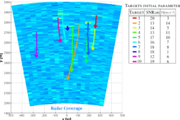
We then consider a typical scenario with10random targets depicted in fig. 4.
Fig. 4. True tracks in the x-y plane. Targets move with near-constant velocity along the paths shown.
The tracks (the means of each set of target samples) produced by the IP-MCMC-PF algorithm over 100 Monte Carlo runs are shown in fig. 5.
Fig. 5. Tracking trajectory. Np = 500 particles, NMCMC = 50MCMC
chains andB= 100burn-in samples.
We then compared the tracking accuracy, the computational cost and the robustness of the three algorithms over 100
Monte-Carlo simulations. The tracking performance is mea-sured in terms of the Root Mean Square Error (RMSE). The results are reported in fig. 6.
Fig. 6. Position RMSE over time for the (a) SIR PF, (b) PMMH and (c) IP-MCMC-PF.
The performance of the methods is also compared via the average RMSE, the tracking loss rate (TLR) and the average CPU time (avg.CPU), which are listed in Table II.
TABLE II
PERFORMANCE COMPARISON AVERAGED OVER100 MCRUNS
Algorithm Np RMSE TLR avg.CPU
(a) SIR PF 500 6.74 [m] 6% 0.5 5000 6.23 [m] 3% 3.8 (b) PMMH 500 5.42 [m] 1% 0.6 5000 4.65 [m] 0% 2.7 (c) IP-MCMC-PF 500 4.84 [m] 0% 0.4 5000 4.61 [m] 0% 0.69
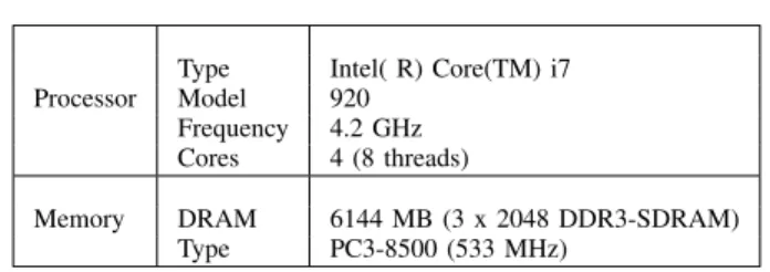
The tracking loss rate (TLR) is defined as the ratio of the number of simulations, in which the target is lost in track (Maximum Position error >20[m]) , to the total number of simulations carried out. The average CPU time (avg.CPU) is the CPU time needed to execute one time step in MATLAB R2011b (win64) on an Intel Core i7 (Nehalem microarchitec-ture) operating under Windows 7 Ultimate (Version 6.1). All the important specifications and features are reported in Table III.
TABLE III SPECIFICATIONS& FEATURES
Processor
Type Intel( R) Core(TM) i7
Model 920
Frequency 4.2 GHz Cores 4 (8 threads)
Memory DRAM 6144 MB (3 x 2048 DDR3-SDRAM) Type PC3-8500 (533 MHz)
VII. CONCLUSION
In this work, we propose an Interacting Population based Monte Carlo Markov Chain based PF (IP-MCMC-PF) that solves the multitarget tracking problem, which is fully par-allelizable. In particular, the proposed algorithm matches the tracking performance of the multitarget SIR PF, while allowing for a dramatic reduction of the computational time.
Furthermore, we demonstrate through simulations that the proposed IP-MCMC-PF provides better tracking performance than the conventional MCMC based particle filter. This holds in terms of track accuracy and robustness to a low number of particles. In fact, sampling particles from the target posterior distribution via interacting population-based simulation avoids sample impoverishment and accelerates the MCMC conver-gence rate.
In a forthcoming work, we will therefore focus on more complex scenarios where targets may enter or leave the observation area. Furthermore, as future research we will investigate the applicability of well known MCMC techniques to additionally reduce the computational burden.
ACKNOWLEDGMENT
The research leading to these results has received funding from the EU’s Seventh Framework Programme under grant agreement no238710.
The research has been carried out in the MC IMPULSE project: https://mcimpulse.isy.liu.se.
REFERENCES
[1] J. Vermaak, S. Godsill, and P. Perez, “Monte carlo filtering for multi-target tracking and data association,”IEEE Tr. Aerospace and Electronic Systems, vol. 41, no. 1, pp. 309–332, January 2005.
[2] D. J. Salmond and H. Birch, “A particle filter for track-before-detect,”
Proc. of the 2001 American Control Conference,, pp. 3755–3760, 2001. [3] C. Kreucher, K. Kastella, and A. Hero, “Tracking multiple targets using a particle filter representation of the joint multitarget probability density,”
Proceedings of the SPIE, vol. 5204, pp. 258–269, 2003.
[4] Y. Boers and J. N. Driessen, “Multitarget particle filter track-before-detect application,” IEE Proc. on Radar, Sonar and Navigation, vol. 151, pp. 351–357, 2004.
[5] A. Doucet and A. M. Johansen, “A tutorial on particle filtering and smoothing: fifteen years later,” In Handbook of Nonlinear Filtering, University Press, 2009.
[6] M. Orton and W. Fitzgerald, “Bayesian approach to tracking multiple targets using sensor arrays and particle filters,”IEEE Transactions on Signal Processing, vol. 50, no. 2, pp. 216–223, February.
[7] C. Andrieu, A. Doucet, and R. Holenstein, “Particle markov chain monte carlo for efficient numerical simulation,”Monte Carlo and Quasi-Monte Carlo Methods, pp. 45–60, Spinger-Verlag Berlin Heidelberg 2008. [8] ——, “Particle markov chain monte carlo methods,”Journal of the Royal
Statistical Society: Series B, vol. 72, no. 3, pp. 269–342, 2010. [9] A. E. Gelfand and A. F. M. Smith, “Sampling-based approaches to
calculaing marginal densities,” Journal of the American Statistical Association, vol. 85, pp. 398–409, 1990.
[10] G. Casella and E. I. George, “Explaining the gibbs sampler,” The American Statistician, vol. 46, no. 3, pp. 167–174, August 1992. [11] N. Metropolis, A. W. Rosenbluth, M. N. Rosenbluth, A. H. Teller, and
E. Teller, “Equations of state calculations by fast computing machines,”
J. Chemical Physics, vol. 21, pp. 1087–1091, 1953.
[12] W. K. Hastings, “Monte carlo sampling methods using markov chains and their applications,”Biometrika, vol. 57, pp. 97–109, 1970. [13] S. Chib and E. Greenberg, “Understanding the metropolis-hastings
algorithm,”The American Statistician, vol. 49, pp. 327–335, 1995. [14] S. Park, J. P. Hwang, E. Kim, and H. J. Kang, “A new evolutionary
particle filter for the prevention of sample impoverishment,” IEEE Transactions on Evolutionary Computation, vol. 13, no. 4, pp. 801–809, August 2009.
[15] W. R. Gilks, S. Richardson, and D. J. Spiegelhalter,Markov Chain Monte Carlo in Practice. Chapman & Hall, 1996.
[16] C. Andrieu and E. Moulines, “On the ergodicity properties of some adaptive mcmc algorithms,”Annals of Applied Probability, vol. 16, no. 3, pp. 1462–1505, 2006.
[17] N. Gordon, D. J. Salmond, and A. F. M. Smith, “Novel approach to nonlinear/non-gaussian bayesian state estimation problems,”IEE Proc. on Radar and Signal Processing, vol. 140(2), pp. 107–113, 1993. [18] A. F. M. Smith and A. E. Gelfand, “Bayesian statistics without tears:
A sampling-resampling perspective,”The American Statistician, vol. 46, pp. 84–88, 1992.
[19] X.-L. Hu, T. Schon, and L. Ljung, “A basic convergence result for particle filtering,” IEEE Transactions on Signal Processing, vol. 56, no. 4, pp. 1337–1348, April 2008.
[20] Z. Khan, T. Balch, and F. Dellaert, “Mcmc-based particle filtering for tracking a variable number of interacting targets,”IEEE Trans. on Pattern Analysis and Machine Intelligence, vol. 27, no. 11, pp. 1805– 1819, 2005.
[21] C. Andrieu and G. O. Roberts, “The pseudo-marginal approach for efficient monte carlo computations,”Annals of Statistics, vol. 37, no. 2, pp. 697–725, 2009.
[22] F. Liang and W. H. Wong, “Real parameter evolutionary monte carlo with applications to bayesian mixture models,”Journal of the American Statistical Association, vol. 96, pp. 653–666, 2001.
[23] A. Gelman and D. B. Rubin, “Inference from iterative simulation using multiple sequences (with discussion),” Statistical Science, vol. 7, pp. 457–511, 1992.