\
Forster, T., Kentikelenis, A. E., Reinsberg, B. , Stubbs, T. H. and King, L.
P. (2019) How structural adjustment programs affect inequality: a
disaggregated analysis of IMF conditionality, 1980–2014.
Social Science
Research
, 80, pp. 83-113. (doi:
10.1016/j.ssresearch.2019.01.001
)
There may be differences between this version and the published version.
You are advised to consult the publisher’s version if you wish to cite from
it.
http://eprints.gla.ac.uk/177675/
Deposited on 11 January 2019
Enlighten – Research publications by members of the University of
Glasgow
How Structural Adjustment Programs Affect Inequality:
A Disaggregated Analysis of IMF Conditionality, 1980–2014
Timon Forster1*, Alexander E. Kentikelenis2, Bernhard Reinsberg3,4, Thomas H. Stubbs3,5, Lawrence P. King6
1 – Freie Universität Berlin, Germany 2 – Bocconi University, Italy
3 – University of Cambridge, United Kingdom 4 – University of Glasgow, United Kingdom
5 – Royal Holloway, University of London, United Kingdom 6 – University of Massachusetts, Amherst, USA
*Correspondence to: [email protected]
Berlin Graduate School for Transnational Studies, Freie Universität Berlin, 14195 Berlin, Germany December 18, 2018
Abstract
This article highlights an important yet insufficiently understood international-level determinant of inequality in the developing world: structural adjustment programs by the International Monetary Fund (IMF). Studying a panel of 135 countries for the period 1980 to 2014, we examine income inequality using multivariate regression analysis corrected for non-random selection into both IMF programs and associated policy reforms (known as ‘conditionality’). We find that, overall, policy reforms mandated by the IMF increase income inequality in borrowing countries. We also test specific pathways linking IMF programs to inequality by disaggregating conditionality by issue area. Our analyses indicate adverse distributional consequences for four policy areas: fiscal policy reforms that restrain government expenditure, external sector reforms stipulating trade and capital account liberalization, financial sector reforms entailing inflation-control measures, and reforms that restrict external debt. These effects occur one year after the incidence of an IMF program, and persist in the medium term. Taken together, our findings suggest that the IMF’s recent attention to inequality neglects the multiple ways through which the organization’s own policy advice has contributed to inequality in the developing world.
Keywords: International Monetary Fund; conditionality; structural adjustment; income inequality; cross-national
JEL codes: F33, F34, F53, O15, O19
Acknowledgements: The authors thank Mark Copelovitch, Adel Daoud, Axel Dreher, Valentin Lang, and participants at both the 2017 Annual Conference on the Political Economy of International Organizations (PEIO) and the 2017 Annual Meeting of the American Sociological Association for insightful comments; the usual caveats apply. Funding by the Institute for New Economic Thinking (INET Grant INO13-00020: ‘The Political Economy of Structural Adjustment’) to support the data collection and from the Cambridge Political Economy Trust / Centre for Business Research at Judge Business School (‘IMF Conditionality and Socioeconomic Development’) is gratefully acknowledged.
1. Introduction
The International Monetary Fund (IMF)—an organization famed for promoting free-market policies around the world—has drawn attention to the perils of income inequality in recent years. Although the IMF issued guidance notes on how to address distributional issues as early as the mid-1990s (IMF 1995; IMF 1996 cited in IMF 2014), the organization has only lately focused on the negative economic consequences of excessive inequality (e.g., Dabla-Norris et al. 2015; Ostry, Berg, and Tsangarides 2014; Ostry, Loungani, and Furceri 2016; IMF 2017). Yet, critics question the Fund’s commitment to reducing income inequality in view of their scant operational changes (Bretton Woods Project 2016; Nunn and White 2016).
Recent estimates show that three out of four households in developing countries live in societies that have become more unequal since the early 1990s (United Nations Development Programme 2013, p. 7). Although income growth in selected populous countries (e.g., China and India) has narrowed the global income distribution, inequality has increased within approximately two-thirds of countries between 1988 and 2011 (Milanovic and Roemer 2016). As these increases in inequality were taking place, international financial institutions (IFIs) were altering national institutions and policies in many developing countries (Babb and Kentikelenis 2018). This occurred through so-called structural adjustment programs: policy-reform packages designed to fundamentally transform a country’s policy arrangements. Among IFIs, the IMF stands out due to its ability to mandate far-reaching policy reforms (known as ‘conditionality’) in borrowing countries (Babb 2005; Copelovitch 2010a; Woods 2006). The socio-economic consequences of these reforms are extensive—ranging from economic growth (Dreher 2006; Vreeland 2003) to reductions in the public sector wage bill (Rickard and Caraway 2018), and from environmental degradation (Shandra, Shircliff, and London 2011) to reductions in health expenditures (Stubbs et al. 2017; Stubbs and Kentikelenis 2018a). Could it be that some of the IMF’s mandated policies adversely affect the income distribution in developing economies?
While previous research shows that IMF structural adjustment programs increase income inequality (Garuda 2000; Lang 2016; Oberdabernig 2013; Pastor 1987; Vreeland 2002), these studies do not identify how these effects work. This study is—to our knowledge—the first to open the black-box of IMF programs and examine the pathways through which their policy reforms operate. Exploiting a newly constructed database on IMF conditionality (Kentikelenis, Stubbs, and King 2016), we empirically test the impact of IMF programs and conditionality on yearly changes in the Gini coefficient of disposable income using panel data for 135 low- and middle-income countries between 1980 and 2014. In so doing, we correct for selection bias into IMF programs and endogeneity of conditionality. Our analysis reveals that four types of IMF-mandated policy conditions exacerbate income inequality: fiscal policy reforms curtailing government expenditure, external sector reforms stipulating trade and capital account liberalization, financial sector reforms entailing inflation-control measures, and conditions restricting external debt. Our findings suggest that these effects occur in the year following the incidence of an IMF program, and also persist in the medium term. These results extend the literature on the socio-economic impact of IMF lending programs, detailing four issue areas of particular concern for income distribution. In doing so, the study demonstrates how international institutions may be an important international-level determinant of income inequality in developing countries.
2. Income Inequality and IMF Conditionality
A voluminous body of literature highlights the adverse social, economic, and political consequences of increased inequality (e.g., Atkinson 2015; Dabla-Norris et al. 2015; Stiglitz 2012; Wilkinson and Pickett 2010). Yet, cross-national research on the causes of income inequality remains limited (for an exception, see Jaumotte, Lall, and Papageorgiou 2013). Recent work has drawn attention to its political and institutional sources (Brady, Blome, and Kleider 2016), and IFI-mandated structural adjustment
programs are one such potential explanatory factor (e.g., Oberdabernig 2013). Enjoying almost universal membership and a global reach through its lending arrangements, the IMF is one of the most powerful IFIs (Woods 2006). As an international lender of last resort, the Fund provides financial assistance to countries in need in exchange for the implementation of policy reforms (or ‘conditionality’). The extent of conditionality—often entailing free-market policies such as stabilization, liberalization, privatization, and deregulation—implies multiple pathways through which IMF programs impact income distribution (Kentikelenis, Stubbs, and King 2016; Stubbs and Kentikelenis 2018b; Woods 2006).
Previous quantitative studies show that on aggregate IMF programs have adverse distributional consequences (Garuda 2000; Lang 2016; Oberdabernig 2013; Pastor 1987; Vreeland 2002). Comparing various economic measures before and after an IMF program, Pastor (1987) finds a reduction in the labor share of income in 18 Latin American economies. Similarly, Vreeland (2002) establishes that the income share of labor in the manufacturing sector decreases in countries with IMF programs. Garuda (2000) also shows that IMF programs are associated with higher Gini coefficients for 39 countries in the period 1975 to 1991. More recently, Oberdabernig (2013) deploys Bayesian Averaging of Classical Estimates to assess the impact of IMF programs on poverty and income inequality, finding that IMF programs increase inequality overall but lower inequality over the sub-period 2000 to 2009. Finally, Lang (2016) demonstrates that IMF programs increase the Gini coefficient of disposable income in democratic countries, but not in non-democratic countries.
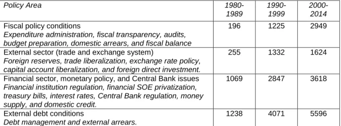
These studies identify the aggregate effect of IMF programs—that is, the impact of financial support, heightened technical assistance, and the multiple components of structural adjustment attached to its lending. Yet, recent evidence on IMF programs and public sector reforms demonstrate that policy outcomes vary based on the specific policy areas under reform (Rickard and Caraway 2018). What IMF conditions might be most likely to affect inequality? This analysis focuses on reforms that plausibly impact the income distribution in the short-run.1 We therefore propose four pathways through which IMF conditionality affects the Gini coefficient of disposable income: fiscal policy issues, external sector conditionality, financial sector reforms; and external debt issues. Box 1 describes these policy areas in detail and provides examples from IMF lending programs.
Box 1: IMF Policy Reforms
1. Fiscal issues pertain to expenditure administration, fiscal transparency, audits, budget preparation, domestic arrears, and fiscal balance. For example, an IMF program with El Salvador in 1993 encompassed quarterly limits on ‘central government total expenditure’ (IMF 1993, p. 11); and a program in 2006 required Turkey to implement a ‘[c]eiling on consolidated primary spending of central government budget and social security institutions’ (IMF 2006, p. 75). 2. External sector reforms refer to the trade and exchange system, including trade liberalization,
exchange rate policy, capital account liberalization, foreign direct investment, and foreign reserves. For example, in 1990 the government of Niger ‘discontinued the system of import and export licenses’ and committed to reducing ‘the number of prohibited imports from three to one’ by the end of the year (IMF 1990, pp. 22-23); and Sri Lanka, in 2001, had to ‘[s]hift to a flexible exchange rate regime’ in order to qualify for financial assistance (IMF 2001a, p. 67).
3. Financial sector conditions encompass reforms related to financial institution regulation, financial state-owned enterprises privatization, treasury bills, interest rates, Central Bank regulation, money supply, and domestic credit. For example, the lending agreement with Guatemala included quantitative ceilings on the growth rate in bank liabilities to the private sector, domestic credit, and credit to public sector (IMF 1983a, p. 28); and the IMF mandated
1 Structural adjustment that takes several years to translate into changes in the income distribution, such as
Uganda to ‘[p]rivatize [the] Uganda Development Bank’ (IMF 2002, p. 68) since it would ‘provide an important source of credit to private sector clients’ (ibid, p. 28).
4. External debt issues are concerned with debt management and external arrears. For example, an IMF program in 1983 instructed Uruguay that, in order ‘[t]o improve the maturity profile of the external debt, the net increase in the external debt of the public sector with original maturities of one year or less (…) is not to exceed US$50 million through end-March 1985’ (IMF 1983b, p. 37); and IMF-designed reforms for Indonesia in 1998 included criteria to limit ‘the contracting or guaranteeing by the non-financial public sector of new nonconcessional external debt with an original maturity of more than one year’ (IMF 1998, p. 14).
Note: Definition of policy areas based on Kentikelenis, Stubbs, and King 2016. See Appendix A for further information.
First, fiscal consolidation measures—entailing policy reforms that lower government expenditure—are a cornerstone of IMF structural adjustment programs. These measures have already been linked to higher inequality independent of IMF programs (Agnello and Sousa 2014; Ball et al. 2013; Mulas-Granados 2005; Schaltegger and Weder 2014; Woo et al. 2013). In particular, fiscal consolidation lowers the wage share due to cuts in public sector wages or unemployment resulting from declined economy activity (Agnello and Sousa 2014; Ball et al. 2013; Woo et al. 2013). In both cases, the poor are potentially disproportionately vulnerable because wages are their main source of income and they are most susceptible to layoffs, respectively. In addition, cuts in social spending increase the Gini coefficient of disposable income since low-income households depend on these government transfers (Mulas-Granados 2005; Schaltegger and Weder 2014). Thus, fiscal conditions may increase the Gini coefficient of disposable income where low-income households disproportionately bear the brunt of reductions in public spending.2
Second, with regard to the external sector policy reforms, the Fund has repeatedly argued for fewer restrictions on goods and capital flows as part of its structural adjustment programs. Especially for (relatively labor-abundant) developing countries, proponents of trade liberalization argue that the removal of trade barriers lowers income inequality as the volume of trade increases and living conditions of employees in exporting sectors improve. In general, these gains are conditional on the terms of trade that different strata of the population face, and so their realization is contextual (Rodrik 2011). For instance, trade liberalization in Latin America often involved removing protections from unskilled-labor intensive sectors, thereby reducing the price of that labor and increasing income inequality (Goldberg and Pavcnik 2004, p. 12). More broadly, studies find that trade exacerbates income inequality for some groups of countries (Bergh and Nilsson 2010; Dreher and Gaston 2008; Goldberg and Pavcnik 2007; Meschi and Vivarelli 2009). Economic openness may also mediate the impact of other determinants of income inequality, such as ethno-linguistic fractionalization (Sturm and De Haan 2015). In addition, policies promoting international economic openness are negatively related to worker rights, further distorting the income distribution (Blanton and Peksen 2016).
Liberalizing capital accounts—another key element of many IMF programs—facilitates foreign direct investment (FDI) and portfolio investment. FDI has been associated with higher economic growth and improved human capital formation. Yet, financial development and capital account liberalization tends to favor the top of the income distribution and increase inequality (Furceri and Loungani 2018; Goldberg and Pavcnik 2004; Roine, Vlachos, and Waldenström 2009). Portfolio investment potentially increases market volatility and amplifies financial crises (McKinnon and Pill 1996), which—when followed by economic downturns—may harm low-income individuals the most (De Haan and Sturm
2 Instead of reducing expenditure, the government may increase taxes, or raise revenue by privatisation of
state-owned enterprises. However, the analysis of their distributional effects is complex (Birdsall and Nellis 2003; Claessens and Perotti 2007). Further, since the effects may take several years to translate into changes of the income distribution, these dimensions of fiscal consolidation are beyond the scope of this article.
2017). For instance, the Asian financial crisis illustrates how foreign capital flows aggravated structural problems of these economies (Corsetti, Pesenti, and Roubini 1999; Furman and Stiglitz 1998). Thus, financial liberalization tends to be associated with higher income inequality (Jaumotte and Osuorio Buitron 2015; Ben Naceur and Zhang 2016; for an opposing view see Agnello, Mallick, and Sousa 2012). In sum, we expect trade and capital account liberalization to widen the income distribution through multiple channels, which suggests potential benefits of external sector reforms accrue predominantly to individuals located at the top of the income distribution.
Third, the Fund typically calls for reforms on monetary policy, initiates the privatization of financial institutions, and specifies targets for the inflation rate. These measures are aimed at stabilizing the financial sector; and, indeed, IMF arrangements diminish the probability of currency crises and reduce inflation (Bird 2007; Dreher and Walter 2010). Yet, combating inflation is not without distributional consequences. When central banks raise interest rates, creditors—as opposed to debtors—stand to benefit; and debtors are more likely to consist of the poor, thereby exacerbating inequalities. More generally, if access to financial services and markets is unequal—as is often the case in developing countries (Claessens and Perotti 2007)—gains of lower inflation or an improvement in investor confidence accrue disproportionately to the rich (De Haan and Sturm 2017). Recognizing the political nature of ‘independent’ monetary institutions (Grabel 2003), some argue that the central banks’ expansionary policy response to the recent financial crisis has further helped those at the top recover the value of their assets (e.g., Stiglitz 2012, p. xi). Taken together, we expect financial sector conditions to increase the income share of individuals located at the higher end of the income distribution, thereby exacerbating income inequality.
Fourth, external debt issues relate to the Fund’s core mandate. Debt management conditions are quantitative criteria limiting the issuance of new external debt. Facing borrowing restrictions, governments may fail to protect social spending, thereby lowering the income share of relatively poor populations. This effect is likely to be compounded in times of crisis, when governments in the developing world already have limited access to finance, and—as a result—cut social expenditure (Wibbels 2006). In addition, external debt conditions may increase the income share of individuals at the top of the income distribution because limits to external debt issuance lead to a higher value of outstanding bonds and a better climate for investments, thereby increasing returns for capital owners. By disaggregating IMF programs, we consider how structural adjustment impacts income inequality; that is, via fiscal policy, external sector, financial sector, and external debt conditions. These reforms tackle economic imbalances in the short-run, so we expect their effects to operate within one year of implementation. Nonetheless, they may persist in the medium term if borrowing countries find it difficult to reverse these reforms. It should also be noted that the mechanisms considered are not necessarily exhaustive. Other policy areas, such as institutional reforms, need not be inequality-neutral. Due to the limited scope of this analysis, we refrain from formulating explicit hypotheses on their impact (see also Appendix A for descriptive information on these policy areas). Nonetheless, we account for alternative policy reforms stipulated by IMF programs empirically.
3. Research Design
3.1 Variables
We investigate the effects of IMF intervention on income inequality for 135 developing countries over the period 1980 to 2014. Appendix B lists all countries included in the study.3 Data on the Gini coefficient of disposable income, which is our measure of within-country income inequality and the
3 We restrict the sample to developing countries because the determinants of income inequality in high-income
countries are different (e.g., see Dabla-Norris et al. 2015; Lang and Mendes Tavares 2018; Milanovic 2016). In robustness checks, we expand the sample to also include advanced nations.
dependent variable, are from the Standardized World Income Inequality Database (SWIID); as are the data on the Gini coefficient of market income, which we use in robustness checks (Solt 2016). Solt exploits systematic relationships among Gini coefficients and employs algorithms for missing data, taking the Luxembourg Income Study as the baseline. In doing so, the SWIID advances on previous data collections in terms of coverage (e.g., Deininger and Squire 1998; Milanovic 2014). Appendix C discusses the dataset in more detail. For additional analyses, we also draw on data on the income share held by the top and bottom quintile of the income distribution, respectively (WDI 2016).
For our key explanatory variables, we use a new dataset of IMF conditionality based on original coding of loan agreements between the Fund and its borrowers (Kentikelenis, Stubbs, and King 2016). Drawing on the Letters of Intent and attached Memoranda of Economic and Financial Policies, Kentikelenis and colleagues extracted the raw text of all conditions and the number of times these conditions were applicable per year—as detailed in Appendix A. The pathways outlined above imply heterogeneous effects of IMF-mandated policy reforms on income distribution. To allow for this, we use different explanatory variables of IMF programs. First, IMF program participation is a binary variable, taking the value of one if an IMF program has been in effect for at least five months in a specific year, and zero otherwise (Dreher 2006). Second, we approximate the intrusiveness and stringency of conditionality by the number of binding conditions (Copelovitch 2010b; Dreher and Jensen 2007; Woo 2013). The disbursement of loans requires implementation of binding conditions, whereas failure to comply with non-binding conditions does not automatically suspend lending (IMF 2001b; Stubbs et al. 2017). When countries fail to implement conditions, program reviews by Fund staff are delayed (or, ‘interrupted’). To account for this, we discount conditions during the interruption period in case of a delayed program review and use this measure as a robustness check.
Control variables are a set of economic and political determinants of inequality. Research suggests that the level of economic development matters. We therefore include GDP per capita (the natural logarithm), a measure of education (based on the average years of schooling), and life expectancy (Bergh and Nilsson 2010; Dreher and Gaston 2008; Lang 2016; Oberdabernig 2013). Moreover, we account for trade (imports and exports in terms of GDP), and foreign direct investment (net capital inflows as a percentage of GDP) as a measure of de facto financial openness (Jaumotte, Lall, and Papageorgiou 2013; Oberdabernig 2013). Inflation reflects monetary policy, while the rate of unemployment is a determinant of inequality that pertains to fiscal policy (Meschi and Vivarelli 2009; Oberdabernig 2013). Political variables include indicators for the orientation of the leading party, and a democracy index for political regime (Lang 2016); left-wing governments and democracies (for both variables indicated by higher numbers) are expected to be less tolerant to income inequality. These are the baseline controls. For robustness checks, we additionally include GDP growth, the Chinn-Ito Index of financial openness, government consumption as a share of GDP, and urban population as a share of total population (Oberdabernig 2013). Appendices D and E provide the definition and summary statistics of the variables, respectively.
3.2 Estimation Techniques
A key methodological challenge to identifying the average treatment effect of IMF-mandated reforms is non-random assignment of both IMF programs and conditionality.4 As is well documented, selection into IMF programs depends on numerous factors, such as economic growth, the level of international reserves, or political regime (Barro and Lee 2005; Moser and Sturm 2011; Przeworski and Vreeland 2000). IMF lending is also a function of the preferences of the Fund’s major shareholders (Dreher and Jensen 2007; Steinwand and Stone 2008). Controlling for economic and political variables that determine participation, as well as country and year fixed effects, in the outcome equation mitigates the
4 In the context of this study, the average treatment effect refers to the difference in average income inequality
problem of endogeneity to a certain extent. However, time-varying, unobservable variables that predict IMF programs and income inequality—e.g., political will or trust (Vreeland 2003, p. 107)—still bias regression estimates. For example, a government that participates in an IMF program in order to gain international support for liberalizing trade and capital accounts might be willing to accept higher levels of inequality.5
Likewise, conditionality itself—i.e., the number of conditions—may be endogenous and invalidate our analysis for multiple reasons. First, selection into conditionality is not random. Reforms mandated by the IMF depend on the political environment. Lending programs for borrowing countries with democratic institutions or presidential systems, as well as upcoming elections, entail less conditionality, for example, because IMF staff recognize that democratic and newly-elected governments face additional policymaking constraints (Rickard and Caraway 2014; Stone 2008). With regard to income inequality, we posit that a similar logic may apply to the allocation of conditions. That is, we expect the Fund to be more lenient towards countries with high income inequality—not necessarily because of distributional concerns per se but to maintain social and political stability, thereby enhancing the prospects of implementation of its structural adjustment reforms. Indeed, the number of conditions and the level of income inequality in low and middleincome countries are negatively correlated (r = -0.149). Such systematic differences between countries that receive more IMF conditions and those that receive fewer conditions causes endogeneity bias; in the case illustrated, the uncorrected estimates of IMF coefficients underestimate the true effect.6 Second, conditions might be endogenous due to omitted variable bias. For instance, it is possible that IMF staff design lending programs as a function of unobservable variables, such as perceived economic outlook of a borrowing country. In addition, preferences regarding income inequality are likely to differ between IMF staff and government officials, as the latter may have an interest in lowering income inequality in view of political stability or upcoming elections. Thus, borrowing countries that select into conditionality may implement policy reforms such that they maintain or even lower the levels of income inequality. In this case, the omitted variable— government preferences—is correlated with selection into conditionality and income inequality. Since the latter association is negative, estimates that suffer from omitted variable bias would underestimate the true effect of IMF programs. Finally, endogeneity may arise from measurement error in the explanatory variables of interest since any systematic measurement ‘noise’ in IMF programs and conditionality is correlated with the error term.
One approach to overcome these issues and obtain consistent estimates is to use an instrumental variable (IV). A valid instrument ought to explain variation in IMF program participation and conditionality respectively (the relevance condition), but must not be correlated with income inequality except through the IMF variable of interest (the exclusion condition). Variables commonly used as IVs in the literature for selection into IMF programs—e.g., voting in the UN General Assembly (Dreher and Jensen 2007) or temporary UN Security Council membership (Dreher, Sturm, and Vreeland 2015)—are not excludable to income inequality. First, voting in the UN General Assembly reflects political preferences and, as such, might be correlated with domestic policies regarding income distribution (Lang 2016). Second, countries tend to receive higher foreign aid following rotation onto the UN Security Council (e.g., Kuziemko and Werker 2006). In turn, this increases resources for the incumbent government to pay civil servants or fund public services (e.g., health or education), thereby potentially lowering
5 Alternatively, one could restrict the sample to include only country-years with IMF programs. However, this
identifies the average treatment effect of the treated (ATET) (Wooldridge, 2010). The ATET can be distinguished from an average treatment effect insofar as the former captures the conditioned effect of IMF intervention. In this case, the results can only be interpreted within the context of country-years with an IMF program, in turn offering a more limited set of policy implications surrounding the design of conditionality.
6 The literature on the reasons of selection into conditionality is inconclusive. Countries may select into certain
conditions to overcome domestic opposition to policy change (e.g., Vreeland 2006), or the Fund may impose these on borrowing countries (e.g., Grabel 2011; Stiglitz 2002).
income inequality. Furthermore, such ‘political’ instruments assume that the Local Average Treatment Effect (LATE) identified is representative of all IMF programs, not just the politically motivated ones (Dreher, Eichenauer, and Gehring, 2018). This invalidates inference if IMF programs are more (or less) effective when politically motivated. Instead, we draw on recent methodological innovations in political science and construct two separate compound instruments (e.g., Lang 2016; Nunn and Qian 2014; Reinsberg et al. 2018; Stubbs et al. 2018). For selection into IMF programs, we interact the mean number of country-specific IMF program participation with the Fund’s budget constraint, approximated by the number of countries with an IMF program in a given year (Vreeland 2003). For conditionality, we interact the mean number of conditions over the sample period with the number of countries under an IMF program (Lang 2016; see also Nelson and Wallace 2017; Reinsberg et al. 2018; Stubbs et al. 2018 for recent applications on the IMF). Using compound instruments is similar to a (continuous) difference-in-difference design: the impact of conditionality on income inequality is compared between country-years with high and low exposure to IMF conditions. We discuss the relevant assumptions in more detail below.
For selection into IMF programs, the relevance condition is satisfied insofar as the IMF signs fewer loan agreements in times of scarce resources (Dreher and Vaubel 2004; Lang 2016; Vreeland 2003). That is, as the number of countries with IMF programs in a given year increases, the Fund’s resources become more constrained and so it tends to sign fewer new lending arrangements. From the perspective of borrowing governments, countries previously under IMF programs are more likely to sign arrangements again (Bird, Hussain, and Joyce 2004). The country-specific mean of number of years with IMF program participation over the sample period therefore approximates the general propensity of a country to participate in an IMF program in a given year, after controlling for observable factors that usually explain such variation. Thus, the interaction of the number of countries participating in IMF programs and the country-specific probability of participation can predict selection into IMF programs. Essentially, the compound instrument combines exogenous information on the supply of the Fund’s lending programs with country-specific data pertaining to the demand for financial resources from the IMF.
For selection into conditionality, our reasoning is similar. The Fund assigns a higher number of conditions to borrowing countries as the budget constraint becomes binding (Dreher and Vaubel 2004; Lang 2016; Stubbs et al. 2018; Vreeland 2003)—as shown in Figure 1, which plots the number of countries with an IMF program in a given year against the mean number of binding conditions. In years where many countries require financial assistance by the IMF, programs entail more conditions to balance the increased demand in view of limited resources. Further, the mean number of conditions in IMF programs over the entire period captures the country-specific exposure to IMF conditionality. This exposure partly determines the bargaining position of government interlocutors in negotiations with the IMF and more broadly informs future IMF programs. As a result, the compound instrument predicts variation in IMF conditionality.
Source: Authors
Our instruments are also excludable to the extent that variables correlated with the number of countries under programs do not affect inequality differently in low- versus high-exposure recipients of IMF programs or conditionality, conditional on country and year fixed effects and other controls (Lang 2016; Stubbs et al. 2018).7 For example, global financial crises would increase demand for IMF lending and thus the number of countries under program. However, given the inclusion of year fixed effects and a battery of other control variables, it is unlikely that global financial crises alter the effect of IMF treatments in low- versus high-exposure recipients of IMF treatments. We cannot think of any other variable that would mediate the impact of the Fund’s budget constraint on income inequality.
We implement this identification strategy by using maximum likelihood estimation over a system of three equations, thereby addressing the endogeneity of IMF programs and conditionality with a two-stage least-squares IV approach:
𝐼𝑀𝐹
̂𝑖𝑡 = 𝛼0+ 𝛼1(𝐼𝑀𝐹̅̅̅̅̅̅𝑖× 𝐵𝑢𝑑𝑔𝑒𝑡𝑡)𝑡−1+ 𝛼2′𝑋𝑖𝑡−1+ 𝛾′𝑍𝑖𝑡−1+ 𝜌𝑖+ 𝜈𝑡 (1)
𝐶𝑜𝑛𝑑̂𝑖𝑡 = 𝜋0+ 𝜋1(𝐶𝑜𝑛𝑑̅̅̅̅̅̅̅𝑖× 𝐵𝑢𝑑𝑔𝑒𝑡𝑡)𝑡−1+ 𝜋2′𝑋𝑖𝑡−1+ 𝜇𝑖+ 𝜈𝑡 (2)
𝐺𝑖𝑛𝑖𝑖𝑡 = 𝛽0+ 𝛽1𝐼𝑀𝐹̂𝑖𝑡−1+ 𝛽2𝐶𝑜𝑛𝑑̂𝑖𝑡−1+ 𝛽3′𝑋𝑖𝑡−1+ 𝜇𝑖+ 𝜈𝑡+ 𝜀𝑖𝑡 (3)
where 𝑖 denotes a country and 𝑡 a year. Equation 3 is the outcome equation explaining the Gini coefficient of disposable income. 𝐼𝑀𝐹̂ and 𝐶𝑜𝑛𝑑̂ are the fitted values from the selection equations 1 and 2, respectively. The total number of conditions approximates structural adjustment, whereas the coefficient on the IMF participation dummy reflects the marginal effect on income inequality beyond the number of conditions. For instance, one could think of the Fund’s technical assistance or catalytic effects on aid (Stubbs, Kentikelenis, and King 2016), which are—to a degree—independent of program specifics. 𝑋 denotes a vector of control variables, as discussed above. Any effect of IMF arrangements
7 Bun and Harrison (2018) and Nizalova and Murtazashvili (2016) provide analytical proofs that the interaction
of an endogenous variable (i.e., the country-specific exposure to IMF programs) with an exogenous one (i.e., the Fund’s budget constraint, or the number of countries under programs) can be interpreted as being exogenous.
and the control variables on income inequality is unlikely to materialize instantaneously. To allow for a delayed effect, we lag the explanatory variables by one period (e.g., Oberdabernig 2013; Vreeland 2002). The model controls for time-invariant country-specific variables, 𝜇, and year fixed effects, 𝜐. In addition, we compute heteroscedasticity-robust standard errors and cluster them on the country-level to account for autocorrelation within countries.
Equation 1 explains IMF program participation as a function of the lagged compound instrument, 𝐼𝑀𝐹
̅̅̅̅̅̅ × 𝐵𝑢𝑑𝑔𝑒𝑡. In addition, we include the vector of controls from the outcome equation, 𝑋, and a
vector of lagged explanatory variables specific to selection into IMF programs, 𝑍 (e.g., Barro and Lee 2005, Kentikelenis, Stubbs, and King 2015). We account for economic variables—GDP per capita, GDP growth, reserves, and current account balance—as well as relevant political variables—an index for democracy, and binary variables for legislative and executive elections. Moreover, we control for past participation because countries previously under IMF programs are more likely to sign arrangements again (Bird, Hussain, and Joyce 2004). The compound instrument therefore captures only variation in IMF programs due to the Fund’s budget constraint and the country-specific probability, net of these controls.8 We further include regional fixed effects, 𝜌, and as in Equation 3, we also control for year fixed effects, 𝜐.
In Equation 2, we derive the predicted number of conditions drawing on our compound instrument, 𝐶𝑜𝑛𝑑
̅̅̅̅̅̅̅ × 𝐵𝑢𝑑𝑔𝑒𝑡. This selection equation also includes the controls of Equation 3, 𝑋, country dummies,
𝜇, and year fixed effects, 𝜐. To implement these analyses, we estimate a multi-equation econometric model with a structure of correlated errors that are assumed to be jointly normally distributed (Roodman 2011).9
For subsequent analyses of the policy reforms discussed, we use the number of conditions covering a specific policy area—as opposed to the total number of conditions—alongside the number of remaining conditions (the latter corresponds to the total number of conditions minus the number of conditions in the policy area of interest). Failure to account for all components of IMF programs causes omitted variable bias (i.e., the policy area of interest partly captures the impact of the remaining conditions due to collinearity). Following the instrumentation strategy described above, we interact the within-country mean exposure to the policy area of interest with the Fund’s budget constraint from the previous period to obtain an IV.10 Since conditionality impacts the income distribution indirectly through macroeconomic variables, the inclusion of these absorbs variation in the dependent variable and therefore corresponds to a very stringent test of the IMF’s impact on income inequality.
4. Results
4.1 Illustrative Evidence
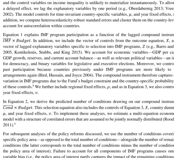
In this section, we provide some descriptive information on our main explanatory variables of interest. Table 1 summarizes the Gini coefficient of disposable income and the IMF measures of interest in our sample of 135 developing countries in years with IMF programs. External debt and financial sector
8 In Appendix G10, we report baseline results when excluding the vector of controls specific to the selection into
IMF programs. As expected, the compound instrument is stronger—as indicated by the Kleibergen-Paap statistics—but the estimate of the coefficient on IMF program participation remains insignificant. The results regarding the IMF variables of interest, i.e., the total number of conditions and policy areas under consideration, are substantively the same as in our main analysis.
9 For the technical details on estimating the system of three equations, see Roodman (2009).
10 We do not instrument for the remaining number of conditions since we are interested in measuring the effect of
the policy area of interest, controlling for the actual, rather than the predicted features of lending programs. In addition, instrumenting for the remaining number of conditions would lead to less precise estimates because of potential issues of multicollinearity and it is computationally expensive due to the higher number of parameters to be estimated.
conditions are most frequently incorporated in lending arrangements, which reflects the IMF’s core areas of capabilities and mandate. Nonetheless, even fiscal policy conditions and external sector reforms feature prominently in IMF programs.
Table 1: Descriptive statistics: Gini coefficient and IMF measures
Variable N Mean Median S.d. Min Max
Gini coefficient of disposable income 1223 40.738 39.894 6.709 22.773 57.085
Total conditions 1223 23.412 24 15.976 0 124
Fiscal policy conditions 1223 3.450 2 3.911 0 21
External sector conditions 1223 2.523 3 2.484 0 24
Financial sector conditions 1223 5.940 6 4.773 0 36
External debt conditions 1223 8.697 9 6.090 0 40
In Table 2, we present the correlation matrix of the variables discussed. It is noteworthy that all IMF measures of interest except financial sector conditions are negatively correlated with income inequality. This is consistent with our potential source of endogeneity discussed in Section 3.2—that countries with relatively high levels of inequality tend to receive fewer conditions. Thus, estimates uncorrected for endogeneity potentially underestimate the adverse distributional consequences. As the correlation matrix further illustrates, the correlation between policy reforms is highest for external debt conditions and financial sector reforms, which is expected given their frequency presented in Table 1.
Table 2: Correlation matrix: Gini coefficient and IMF measures
Gini coeff. Total cond. Fiscal policy External sector Financial sector External debt
Gini coefficient of disposable income 1
Total conditions -0.131 1
Fiscal policy conditions -0.185 0.648 1
External sector conditions -0.036 0.695 0.267 1
Financial sector conditions 0.015 0.787 0.269 0.593 1
External debt conditions -0.076 0.870 0.493 0.546 0.664 1
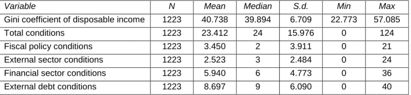
Next, we provide illustrative evidence of the distributional consequences of exposure to IMF conditionality. To approximate the latter, we calculate the total number of conditions in the four policy areas of interest by country from 1980 through 2014, and assign countries to the corresponding quintiles. Then, Figure 2 plots the mean Gini coefficient for countries in the bottom (Q1) and top (Q5) quintile of IMF conditionality in fiscal policy issues (FP), external sector conditions (EXT), financial sector reforms (FIN), and external debt issues (DEB) from locally weighted scatterplot smoothing (bandwidth is 20 percent). For fiscal policy issues (the short-dashed lines), the trends in income inequality clearly diverge: Countries with high exposure to these conditions have experienced an increase in the Gini coefficient over the time considered, while their level remains below low-exposure countries throughout. The differences in the trajectory are less pronounced for external sector conditions (the long-dashed lines), financial sector reforms (the solid lines), and external debt issues (the dot-dashed lines). In all cases, high exposure to IMF conditionality is weakly associated with a decrease in the Gini coefficient. In addition, countries in the top quintile of conditions tend to have lower levels of income inequality.
Figure 2: Gini coefficient by exposure to conditionality in selected policy areas
Source: Authors
Taken together, the illustrative evidence provides only tentative support for the mechanisms discussed in Section 2. We find that the association of fiscal issues with income inequality indicates adverse distributional consequences, whereas conditions in the other three policy areas tend to lower the Gini coefficient of disposable income—although the changes are smaller in magnitude. In addition, it is noteworthy that for all policy areas of interest, countries with relatively high levels of income inequality receive fewer conditions—as discussed in Section 3.2 regarding potential endogeneity bias. Of course, Figure 2 presents an incomplete picture of IMF programs, e.g., since the data is aggregated and only a number of countries are considered. Further, the association is merely descriptive because we do not control for any confounding variables. Thus, to better understand the causal impact of IMF programs on income inequality, we now present the results from regression analyses.
4.2 Multivariate analysis
In Table 3, we present our baseline quantitative analyses. Specification 1 only accounts for the macroeconomic determinants of income inequality. Most of these control variables are statistically insignificant—partly due to country and year fixed effects, and country-clustered standard errors. Yet, the signs of the coefficients largely conform to established theories. GDP per capita (p<0.01), inflation (p<0.001), and the rate of unemployment (p<0.05) are all positively correlated with the Gini coefficient. Life expectancy is also associated with higher income inequality; however, the coefficient is statistically insignificant and sensitive to the model specification. By contrast, countries with higher average education tend to have lower income inequality. Likewise, we find that income inequality is associated with decreases in external sector measures—trade and FDI. Finally, left-leaning governments and democratic institutions are associated with lower levels of income inequality, all else being equal. However, all these coefficients are estimated less precisely, and we fail to reject the null hypothesis of no effect at standard levels of statistical significance.
Table 3: Baseline model
Specification 1 2 3 4 L. IMF program 0.186 0.045 -0.348 [0.418] [0.407] [0.593] L. Total conditions 0.007 0.113** [0.007] [0.042] L. GDP per capita (ln) 7.100** 7.122** 7.162** 8.102*** [2.685] [2.683] [2.673] [2.370] L. Education -2.944 -2.937 -2.984 -3.679 [2.328] [2.327] [2.320] [2.466] L. Trade -0.021 -0.021 -0.021 -0.018 [0.012] [0.013] [0.013] [0.014] L. FDI -0.007 -0.007 -0.007 -0.005 [0.021] [0.021] [0.021] [0.024] L. Inflation 0.001*** 0.001*** 0.001*** 0.001** [0.000] [0.000] [0.000] [0.000] L. Unemployment 0.142* 0.137* 0.137* 0.104 [0.070] [0.070] [0.069] [0.069] L. Life expectancy 0.022 0.02 0.016 -0.053 [0.083] [0.082] [0.082] [0.087] L. Govt. orientation -0.097 -0.095 -0.1 -0.13 [0.133] [0.135] [0.135] [0.164] L. Democracy index -0.027 -0.03 -0.028 -0.023 [0.110] [0.111] [0.110] [0.105]
Country fixed effects Yes Yes Yes Yes
Year fixed effects Yes Yes Yes Yes
F-statistic IMF program - 23.77 23.70 54.55
F-statistic conditionality - - - 30.63
N 987 987 987 987
Notes: F-tests are Kleibergen-Paap Wald statistics for compound instruments. Cluster robust standard errors in brackets. * p<0.05, ** p<0.01, *** p<0.001
Specification 2 incorporates the endogeneity-corrected binary indicator for an IMF program. The control variables remain unchanged. The coefficient on the binary IMF variable is positive, indicating that IMF programs overall increase the Gini coefficient. However, unlike previous research, we find that this effect is not significantly different from zero at conventional thresholds.
To disentangle the potentially heterogeneous effects of IMF programs, Specification 3 and 4 additionally control for the count of conditions. Specification 3 does not correct for the endogeneity of conditionality. The estimated effect of the total number of conditions is positive, but close to zero, which is consistent with the sources of bias described above. In Specification 4, we use compound instrumentation for the total number of conditions such that all IMF measures lend themselves to causal interpretation. The binary IMF indicator—now reflecting aspects of programs beyond conditionality— has turned negative, but remains insignificant. By contrast, the number of total conditions is positive and significant (p<0.01). For one additional binding condition, the Gini coefficient increases by 0.113,
ceteris paribus. At the mean number of binding conditions (considering all country-years with IMF programs in our sample of developing countries), 23.4, this amounts to an increase of the Gini by 2.644 points. The impact of conditionality is therefore also substantively meaningful; Gini coefficients in our data range from a minimum value of 22.773 to a maximum of 57.085, with a standard deviation of 6.709. These inferences hinge on the assumption that our identification strategy is valid. Thus, we
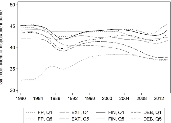
present the first-stage results from predicting IMF program participation (Specification 4a) and the total number of condition (Specification 4b) in Table 4.
The estimates for selection into IMF programs (Specification 4a) are consistent with findings of earlier studies (e.g., see Kentikelenis, Stubbs, and King 2015; Vreeland 2002). Past IMF participation predicts future IMF programs (p<0.001). All other variables are insignificant at standard thresholds, although their sign is mostly as expected: economic growth, higher reserves, and current account balance are all associated with a lower probability of obtaining an IMF program. GDP per capita is estimated with high standard errors because it is included twice, once lagged to predict IMF program participation and once contemporaneously as a control from the outcome equation. Considering political variables, the effect of past elections depends on the type of election, but are both estimated imprecisely. Importantly, our compound instrument is highly significant (p<0.001) and the sign is as expected. Given a number of countries under an IMF program, the country-specific mean participation is positively associated with selection into IMF programs. Put differently, the IMF's response to a more strained budget will be felt proportionally more in countries regularly borrowing from the Fund (i.e., those with high past participation) (Lang 2016).
For selection into conditionality (Specification 4b), we include all control variables from the outcome equation and our compound instrument. The interaction of the country-specific mean number of conditions with the budget constraint is highly significant (p<0.001) and positive, suggesting that for any number of countries under IMF programs, countries obtain more conditions the higher their average exposure to conditionality over the period under consideration. This substantiates our claim regarding the relevance condition because as the number of countries participating in IMF programs increases, the features of past arrangements become increasingly important in informing the design of future programs.
Table 4: First-stage results
Dependent Variable IMF participation Conditionality
Specification 4a 4b L. Instrument IMF 0.011*** [0.001] L. Instrument Conditionality 0.035*** [0.006] L. IMF program 0.359*** [0.030] L. GDP per capita (ln) 0.272 [0.241] L. GDP growth -0.005 [0.003] L. Reserves -0.004 [0.003]
L. Current account balance -0.002
[0.002] L. Democracy index 0.000 [0.018] L. Legislative election 0.006 [0.032] L. Executive election -0.059 [0.040]
Controls from outcome eq. Yes Yes
Region fixed effects Yes No
Country fixed effects No Yes
Year fixed effects Yes Yes
F-statistic IMF program 54.55 -
F-statistic conditionality - 30.63
N 987 987
Notes: F-tests are Kleibergen-Paap Wald statistics for compound instruments. Cluster robust standard errors in brackets. * p<0.05, ** p<0.01, *** p<0.001
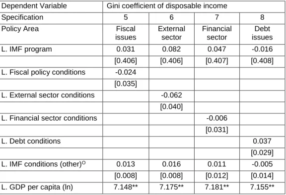
Table 5 shows our quantitative analyses of individual policy areas without instrumentation. As expected, the estimated coefficients of interest without instrumentation are all close to zero, albeit insignificant. This supports our argument regarding endogeneity bias made in Section 3.2. Specifically, when considering the politics of conditionality and looking at the terms of lending programs as the outcome of a bargaining process, government bureaucrats are likely to take into account potential changes to income inequality when selecting into conditionality. As government officials consider upcoming elections or political stability, they are more conscious of distributional consequences of structural adjustment than when conditions are imposed by IMF staff, thereby implementing reforms such that they are inequality-neutral, or inequality-reducing at best. In fact, the estimates for the coefficients on fiscal issues, external sector reforms, and financial sector conditions all indicate that when conditions are endogenous, they lead to lower income inequality—although these estimates are not significant at standard thresholds. The controls remain substantively the same throughout these specifications, and we refrain from discussing these from now on. In Table 6, we present the IV estimates, which we consider more credible since they address the endogeneity of structural adjustment reforms (see Appendix F1 and F2 for first-stage results). The findings with instrumentation support the theoretical expectations outlined earlier, namely, that conditionality pertaining to fiscal constraint (p<0.05), the external sector (p<0.05), the financial sector (p<0.06), and external debt management (p<0.001) increase the Gini coefficient of disposable income. Diagnostic statistics across all specifications indicate that our compound instruments are strong, as suggested by the respective Kleibergen-Paap Wald F-statistics (Staiger and Stock 1997).
Table 5: Policy areas not corrected for endogeneity
Dependent Variable Gini coefficient of disposable income
Specification 5 6 7 8
Policy Area Fiscal
issues External sector Financial sector Debt issues L. IMF program 0.031 0.082 0.047 -0.016 [0.406] [0.406] [0.407] [0.408]
L. Fiscal policy conditions -0.024
[0.035]
L. External sector conditions -0.062
[0.040]
L. Financial sector conditions -0.006
[0.031]
L. Debt conditions 0.037
[0.029]
L. IMF conditions (other)O 0.013 0.016 0.011 -0.005
[0.008] [0.008] [0.012] [0.014]
[2.662] [2.673] [2.677] [2.665] L. Education -2.895 -2.967 -3.047 -3.019 [2.316] [2.300] [2.334] [2.316] L. Trade -0.021 -0.021 -0.02 -0.021 [0.013] [0.013] [0.013] [0.013] L. FDI -0.007 -0.007 -0.007 -0.007 [0.021] [0.021] [0.021] [0.021] L. Inflation 0.001*** 0.001*** 0.001*** 0.001*** [0.000] [0.000] [0.000] [0.000] L. Unemployment 0.139* 0.135* 0.137* 0.137* [0.070] [0.068] [0.069] [0.068] L. Life expectancy 0.015 0.015 0.016 0.014 [0.082] [0.082] [0.082] [0.081] L. Govt. orientation -0.112 -0.105 -0.097 -0.095 [0.132] [0.136] [0.134] [0.136] L. Democracy index -0.028 -0.027 -0.031 -0.037 [0.109] [0.110] [0.109] [0.108]
Country fixed effects Yes Yes Yes Yes
Year fixed effects Yes Yes Yes Yes
F-statistic IMF program 23.72 23.74 23.75 23.67
F-statistic conditionality - - - -
N 987 987 987 987
Notes: F-tests are Kleibergen-Paap Wald statistics for compound instruments. Cluster robust standard errors in brackets. O This variable corresponds to the total number of conditions minus the number of conditions in the
policy area of interest tested in this model. * p<0.05, ** p<0.01, *** p<0.001.
Table 6: Policy areas corrected for endogeneity
Dependent Variable Gini coefficient of disposable income
Specification 9 10 11 12
Policy Area Fiscal
issues External sector Financial sector Debt issues L. IMF program 0.034 -0.137 -0.146 -0.429 [0.459] [0.485] [0.513] [0.624]
L. Fiscal policy conditions 0.495*
[0.233]
L. External sector conditions 0.836*
[0.366]
L. Financial sector conditions 0.521
[0.272]
L. Debt conditions 0.481***
[0.146]
L. IMF conditions (other)O 0.012 0.013 0.01 -0.01
[0.008] [0.007] [0.012] [0.014]
L. GDP per capita (ln) 7.968** 7.903*** 7.628** 8.387***
[2.559] [2.339] [2.333] [2.191]
L. Education -4.604 -3.736 -1.826 -4.373
L. Trade -0.011 -0.018 -0.022 -0.018 [0.015] [0.014] [0.014] [0.015] L. FDI -0.007 0.002 -0.001 -0.011 [0.024] [0.029] [0.030] [0.028] L. Inflation 0.001* 0.001* 0.001* 0.001*** [0.000] [0.000] [0.000] [0.000] L. Unemployment 0.084 0.121 0.082 0.089 [0.070] [0.076] [0.081] [0.067] L. Life expectancy -0.036 -0.049 -0.06 -0.104 [0.089] [0.086] [0.096] [0.095] L. Govt. orientation 0.036 -0.069 -0.218 -0.049 [0.215] [0.161] [0.156] [0.193] L. Democracy index -0.024 -0.041 0.051 -0.128 [0.123] [0.115] [0.111] [0.101]
Country fixed effects Yes Yes Yes Yes
Year fixed effects Yes Yes Yes Yes
F-statistic IMF program 32.73 44.47 43.79 51.20
F-statistic conditionality 11.91 16.45 10.82 18.40
p value conditions 0.0383 0.0244 0.0597 0.0012
N 987 987 987 987
Notes: F-tests are Kleibergen-Paap Wald statistics for compound instruments. ‘p value conditions’ refers to a Wald test of equivalence between the coefficient on the policy area of interest and all other conditions. Cluster robust standard errors in brackets. O This variable corresponds to the total number of conditions minus the number
of conditions in the policy area of interest tested in this model. * p<0.05, ** p<0.01, *** p<0.001.
First, one additional fiscal policy condition increases the Gini coefficient of disposable income by 0.495 points, ceteris paribus (p<0.05)—and this effect is different from the remaining number of conditions (Wald test of equivalence of coefficients, p<0.04). In our sample of IMF programs, 58.0 percent include at least one fiscal policy condition. Their mean is 3.5, implying an increase of the Gini coefficient by 1.733 points, all else being equal.
Second, we find that external sector conditions lead to a rise in the Gini coefficient (p<0.05). On average, one external sector condition increases the Gini index by 0.836, and this point estimate is statistically different from the estimated coefficient on the remaining number of conditions (Wald test of equivalence of coefficients, p<0.03). Similar to fiscal issues, 58.5 percent of IMF programs with emerging and developing countries over the period from 1980 to 2014 include at least one external sector reform. At the mean of 2.5 conditions, the predicted change in income inequality is 2.090. Third, we find statistically weak evidence that financial sector conditionality also increases the Gini coefficient (p<0.06), and we reject the null hypothesis of equivalence with the remaining number of conditions at the 6 percent level. The estimate corresponds to an increase of the Gini coefficient by 0.521 per condition. Almost four in five country-years with IMF lending (or 78.0 percent) entail financial sector reforms. Given an average of 5.9 financial sector conditions per IMF program, this type of conditionality is predicted to increase the Gini coefficient by 3.074.
Fourth, one additional external debt condition is associated with an increase in income inequality by 0.481 (p<0.001). As discussed above, conditions of this policy area have the highest mean with 8.7 conditions. This translates into an average increase of the Gini coefficient by 4.185 points. Furthermore,
its impact is statistically significantly different from all other conditions (Wald test of equivalence of coefficients, p<0.01).11
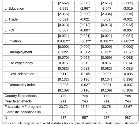
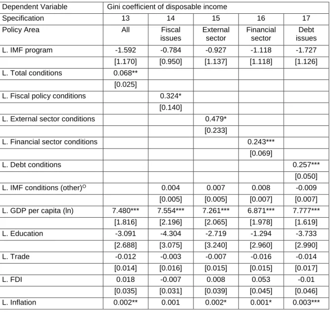
Thus far, the analyses consider year-to-year changes in the Gini coefficient of disposable income. Yet, within-country income inequality is a persistent phenomenon. Thus, we further examine the distributional consequences of IMF programs in the medium term. Towards this end, we collapse the data into non-overlapping three-year periods.12 As a result, the sample size decreases by more than 50 percent to 452 observations. Table 7 depicts that the detrimental impact of IMF conditionality persists in the medium term across all policy areas considered. The estimated coefficients are all statistically different from the remaining number of conditions. However, also note that the instrumentation is slightly weaker, particularly for financial sector conditions and external debt issues. This is potentially due to lower variation in the IMF measures—an issue one would expect to be most severe in policy areas with a relatively high number of conditions, which lose their discriminatory power when being aggregated over time.
Table 7: Medium-term effects
Dependent Variable Gini coefficient of disposable income
Specification 13 14 15 16 17
Policy Area All Fiscal
issues External sector Financial sector Debt issues L. IMF program -1.592 -0.784 -0.927 -1.118 -1.727 [1.170] [0.950] [1.137] [1.118] [1.126] L. Total conditions 0.068** [0.025]
L. Fiscal policy conditions 0.324*
[0.140]
L. External sector conditions 0.479*
[0.233]
L. Financial sector conditions 0.243***
[0.069]
L. Debt conditions 0.257***
[0.050]
L. IMF conditions (other)O 0.004 0.007 0.008 -0.009
[0.005] [0.005] [0.007] [0.007] L. GDP per capita (ln) 7.480*** 7.554*** 7.261*** 6.871*** 7.777*** [1.816] [2.196] [2.065] [1.978] [1.619] L. Education -3.091 -4.304 -2.719 -1.294 -3.733 [2.688] [3.075] [3.240] [2.960] [2.990] L. Trade -0.012 -0.003 -0.007 -0.016 -0.014 [0.014] [0.016] [0.015] [0.015] [0.017] L. FDI 0.018 -0.007 0.008 0.053 -0.01 [0.035] [0.031] [0.039] [0.045] [0.046] L. Inflation 0.002** 0.001 0.002* 0.001* 0.003***
11For analyses of policy areas not discussed in Section 2, see Appendix G4.
12We average the macroeconomic variables and sum the IMF condition counts over non-overlapping three-year
periods (see also Reinsberg et al. 2018). We recode the IMF program dummy as one if there has been an IMF program in effect for at least five months in any of the three years. Additionally, the values of the binary indicators for legislative and executive elections depend on the last year of each period.
[0.001] [0.001] [0.001] [0.001] [0.001] L. Unemployment 0.006 0 0.037 -0.017 0.003 [0.080] [0.073] [0.096] [0.093] [0.073] L. Life expectancy -0.074 -0.028 -0.069 -0.059 -0.125 [0.083] [0.089] [0.087] [0.079] [0.075] L. Govt. orientation -0.243 -0.049 -0.211 -0.292 -0.274 [0.223] [0.286] [0.221] [0.220] [0.238] L. Democracy index 0.131 0.173 0.106 0.191 -0.059 [0.159] [0.182] [0.191] [0.170] [0.151]
Country fixed effects Yes Yes Yes Yes Yes
Year fixed effects Yes Yes Yes Yes Yes
F-statistic IMF program 43.97 38.18 46.45 43.53 49.58
F-statistic conditionality 11.12 7.42 9.89 6.94 3.89
p value conditions - 0.0231 0.0431 0.0006 0.0000
N 452 452 452 452 452
Notes: tests are Kleibergen-Paap Wald statistics for compound instruments. ‘p value conditions’ refers to an F-test of equivalence between the coefficient on the policy area of interest and all other conditions. Cluster robust standard errors in brackets. O This variable corresponds to the total number of conditions minus the number of
conditions in the policy area of interest tested in this model. * p<0.05, ** p<0.01, *** p<0.001.
Taken together, these results support the pathways discussed above: fiscal issues, external sector conditionality, financial sector reforms, and external debt issues all widen income inequality. Additionally, we show that these effects are strongest in the short term, but persist over three years.
5. Further Analyses
In further analyses, we examine the impact of IMF policy reforms on different segments of the income distribution. Section 2 yields not only predictions about the impact of the policy areas of interest on the Gini coefficient, but also points towards differential consequences for the income share of individuals depending on their position in the income distribution. Thus, we regress the income share of the top and bottom income quintile, respectively, on our IMF measures of interest and the controls—see Appendix G1. Consistent with the pathways discussed, we find that IMF programs overall (p<0.05), external sector reforms (p<0.01), financial sector conditions (p<0.05), and external debt issues (p<0.01) increase the income share of the top quintile. Conversely, we find some evidence that fiscal issues (p<0.06) and external debt issues (p<0.05) widen income inequality due to declining incomes for the bottom quintile. However, due to the reduced sample of only 481 observations and less variation amongst the predictors, our identification strategy performs slightly weaker than in the baseline models, as evidenced by lower Kleibergen-Paap statistics.
As an additional robustness check, we evaluate the different mechanisms using the Gini coefficient of market income (Solt 2016) in Appendix G2. Examining changes in the Gini coefficient of market income, the estimates are very similar to the results presented in Section 4.2, both in terms of magnitude and level of statistical significance.
Next, we consider an implementation-discounted binding condition count in Appendix G3. The IMF measures of interest are available for a reduced time period, making instrumentation more difficult due to the loss of observations (the sample size decreases by almost 20 percent to 2,285 observations to predict conditionality; 985 observations remain to estimate the outcome equation). In the first-stage equation for the number of conditions, we therefore replace country fixed effects with regional fixed effects. Under the new instrumentation strategy, the exclusion criterion implies that conditional on a country’s mean exposure to IMF programs, and net of all controls, regional and year fixed effects, the
Fund’s budget constraint—determined independent of a given country—affects the income distribution of any economy only through the number of conditions. Thus, time-invariant country characteristics that impact on income inequality potentially bias our results, e.g., institutional quality beyond the regional average. Adopting this instrumentation strategy, the results remain substantively the same. In fact, the point estimates across all policy areas have increased in magnitude. This suggests that implementation of IMF-mandated policy reforms does, on average, adversely affect the income distribution.
As discussed in Section 2, we explicate theoretical mechanisms only for the policy areas that plausibly impact upon income inequality within one year of implementation. In Appendix G4, we perform the same analyses on the remaining number of conditions. We find that labor issues, privatization and reforms of state-owned enterprises, and revenue issues are all insignificant. By contrast, institutional reforms are associated with an increase in the Gini coefficient of disposable income (p<0.01). Yet, this finding is not sensitive to all robustness checks, and because of the relatively small number of binding conditions over the sample period, we leave this for the subject of further investigation.
Our baseline analyses exclude high-income countries since the determinants of income inequality differ from those in the developing world. In Appendix G5, we provide some suggestive evidence that the impact of IMF programs also differs by these country groups. Due to the high number of parameters estimated we cannot perform the analyses on high-income countries alone. Instead, we expand our sample to include all countries in our analyses together—irrespective of their level of development. As a result, the total number of observations increases to 1,990. While the standard errors decrease as consequence, the estimates of the coefficients of interest are also slightly smaller. The total number of conditions (p<0.01), external sector reforms (p<0.05), financial sector conditions (p<0.05), and debt issues (p<0.001) remain significant, while we find weakly significant evidence for the adverse distributional consequences of fiscal issues (p<0.08). Overall, the reduction of the impact on the Gini coefficient considering all countries supports the notion that the dynamics differ by country groups, suggesting that the negative impact of IMF interventions on income inequality are likely to be more pronounced in developing countries.
Another concern to the validity of our analyses may be that we include extensive control variables in the baseline specifications. Some variables potentially control for pathways we are trying to measure. For instance, fiscal issues may impact upon the income distribution in part through changes in unemployment. The inclusion of these controls may therefore give rise to post-treatment bias (Angrist and Pischke 2008). To address these concerns, we perform our analyses on a smaller set of control variables, excluding trade, FDI, unemployment, and inflation in Appendix G6. The results for the total number of conditions (p<0.05), fiscal issues (p<0.001), external sector reforms (p<0.06), and debt issues (p<0.05) remain substantively unchanged. Yet, financial sector conditions now turn insignificant at conventional levels of statistical significance (p<0.15)—possibly due to weak instrumentation.
Further, we extend our control variables with GDP growth, the Chinn-Ito Index of financial openness, government expenditure, and the urban population share. The inclusion of further explanatory variables corresponds to a more stringent test for the effect of IMF programs on income inequality and addresses concerns of omitted variable bias. For instance, the models now control for redistributive efforts of borrowing countries. In Appendix G7, we show that all our findings are robust to these additional controls.
In order to provide additional evidence for the validity of our identification strategy, we use a slightly different instrument. Instead of approximating the Fund’s budget constraint with the number of countries under an IMF program, we use the IMF’s liquidity ratio (the natural logarithm) (Lang 2016). In Appendix G8, we present analyses using this alternative compound instrument for the selection into IMF programs, while maintaining the original computation for the selection into conditionality. The
results remain substantively unchanged, although the level of statistical significance is slightly lower due to higher standard errors.
Following extensive criticism of its handling of the Asian financial crisis of the late 1990s (Babb and Carruthers 2008), the IMF has streamlined conditionality and emphasized local ownership of conditionality (IMF 2009). Thus, the year 2000 might represent a structural break. Indeed, Oberdabernig (2013) finds that IMF programs decrease income inequality in the sub-period 2000-2009. In Appendix G9, we thus include an interaction of the number