Ling Li [email protected] Learning Systems Group, California Institute of Technology, Pasadena, CA 91125, USA
Abstract
A multiclass classification problem can be re-duced to a collection of binary problems with the aid of a coding matrix. The quality of the final solution, which is an ensemble of base classifiers learned on the binary problems, is affected by both the performance of the base learner and the error-correcting ability of the coding matrix. A coding matrix with strong error-correcting ability may not be overall op-timal if the binary problems are too hard for the base learner. Thus a trade-off between error-correcting and base learning should be sought. In this paper, we propose a new mul-ticlass boosting algorithm that modifies the coding matrix according to the learning abil-ity of the base learner. We show experimen-tally that our algorithm is very efficient in op-timizing the multiclass margin cost, and out-performs existing multiclass algorithms such as AdaBoost.ECC and one-vs-one. The im-provement is especially significant when the base learner is not very powerful.
1. Introduction
Many efforts of the machine learning research have been focused on binary classification problems. For a multiclass classification problem with more than two different class labels, it is possible to reformulate it as a collection of binary problems. The most popular ap-proaches are one-vs-all where each class is compared against all others, and one-vs-one where all pairs of classes are compared (Allwein et al., 2000).
Dietterich and Bakiri (1995) and Allwein et al. (2000) unified and generalized most such approaches with correcting codes. In their framework, an error-correcting coding matrix is first given, with each row associated with a class from the multiclass problem.
Appearing in Proceedings of the 23rd International Con-ference on Machine Learning, Pittsburgh, PA, 2006. Copy-right 2006 by the author(s)/owner(s).
Binary classifiers (also called base classifiers) are then learned, one for each column of the matrix, on training examples that are relabeled according to the column. Given an unseen input, the vector formed by the out-puts of the base classifiers is compared with every row of the coding matrix, and the class associated with the “closest” row is predicted as the class of the input. The coding matrix is usually chosen for strong error-correcting ability (Dietterich & Bakiri, 1995). How-ever, strong error-correcting ability alone does not guarantee good learning performance—one important assumption for normal error-correcting codes that er-rors are uncorrelated may not hold for the base classi-fiers (Guruswami & Sahai, 1999). Thus the choice of the coding matrix has to balance the needs of strong error-correction and uncorrelated classifier errors, and is usually problem-dependent (Allwein et al., 2000).
Multiclass boosting algorithms based on
error-correcting codes (Schapire, 1997; Guruswami & Sa-hai, 1999) tackle the error correlation among the base classifiers by deliberately reweighting the training ex-amples. They usually start off with an empty cod-ing matrix and all classes indistcod-inguishable from oth-ers, and then iteratively append columns to the ma-trix and train base classifiers so that the confusion be-tween classes can be gradually reduced. The examples are reweighted in a fashion similar to the weighting scheme in the binary AdaBoost (Freund & Schapire, 1996), aiming at uncorrelated errors. In order to re-duce the confusion between classes as fast as possible, in each iteration, a max-cut problem can be solved so that the “optimal” matrix column is obtained. It is however common that researchers usually do not pursue the “optimal” coding matrix when applying the multiclass boosting algorithms. Instead, some choose the matrix columns at random (Schapire, 1997; Gu-ruswami & Sahai, 1999).1 Although the fact of max-cut being NP-complete prevents an efficient solution, this is not exactly the reason for researchers not us-ing it; after all, many multiclass classification
prob-1
We actually did not find out how Guruswami and Sahai (1999) chose the columns.
lems have less than ten classes, and even some simple heuristic methods can do better in reducing the con-fusion than a random method. It is mostly because that, combined with the boosting algorithm, a max-cut or heuristic method does not improve over a ran-dom one (Schapire, 1997).
In this paper, we discuss why max-cut does not work well with existing multiclass boosting algorithms, and propose a general remedy which leads to a new boost-ing algorithm. We first discuss in Section 2 how Ada-Boost.ECC, a typical multiclass boosting algorithm, can be explained as gradient descent on a margin cost function (Sun et al., 2005). The trade-off between the error-correcting ability and the base learning perfor-mance is then explained. We propose in Section 3 the new algorithm to achieve a better trade-off by modify-ing the codmodify-ing matrix accordmodify-ing to the learnmodify-ing ability of the base learner. In Section 4, our algorithm is tested on real-world data sets with four base learners of various degrees of complexity, and the results are quite promising. Finally we conclude in Section 5.
2. AdaBoost.ECC and Multiclass Cost
Consider a K-class classification problem where the class labels are 1, 2, . . . ,K. The training set containsN examples,{(xn, yn)}Nn=1, wherexnis the input and
yn ∈ {1,2, . . . , K}. To reduce the multiclass problem to a collection ofT binary problems, we use a coding matrix M ∈ {−1,0,+1}K×T (Allwein et al., 2000). A base classifier ft is learned on the relabeled exam-ples{(xn,M(yn, t)) :M(yn, t)6= 0} based on thet-th column of M, and classes that are relabeled as 0 are omitted. The columns of Mare also called partitions (or partial partitions if there are 0’s) since they define the way the original examples are split.
Given an input x, the ensemble output F(x) =
(f1(x), . . . , fT(x)) is computed, and the Hamming de-coding2 (Allwein et al., 2000) is used to predict the label of x. In the most general settings, there is a co-efficient αt for every base classifierft. The Hamming distance betweenF(x) and thek-th rowM(k) is
∆ (M(k),F(x)) = T X t=1 αt 1−M(k, t)ft(x) 2 .
Labelyis predicted ifM(y) has the smallest Hamming distance to F(x).
To correctly classify an example (x, y), we want
∆ (M(y),F(x)) to be smaller than ∆ (M(k),F(x)) for 2We consider base classifiers with outputs in{−1,+1}
(see experiment settings in Section 4). Thus a loss-based decoding is equivalent to the Hamming decoding.
Algorithm 1. AdaBoost.ECC (Guruswami & Sahai, 1999)
Input: A training set{(xn, yn)}Nn=1; number of epochsT
1: Initialize ˜D1(n, k) = 1;F= (0,0, . . . ,0), i.e.,ft= 0
2: fort= 1 toT do
3: Choose thet-th columnM(·, t)∈ {−1,+1}K
4: Ut=PNn=1 PK k=1D˜t(n, k)JM(k, t)6=M(yn, t)K 5: Dt(n) =Ut−1· PK k=1D˜t(n, k)JM(k, t)6=M(yn, t)K
6: Trainfton{(xn,M(yn, t))}with distributionDt
7: εt=PNn=1Dt(n)Jft(xn)6=M(yn, t)K 8: αt= 12ln(ε−1t −1) 9: D˜t+1(n, k) = ˜Dt(n, k)·e− αt 2[M(yn,t)−M(k,t)]ft(xn) 10: end for
11: return the coding matrixM, the ensembleFandαt
anyk6=y. Naturally, we may define the margin of the example (x, y) for class k as the difference between these two distances,
ρk(x, y) = ∆ (M(k),F(x))−∆ (M(y),F(x)). (1)
A learning algorithm should pick a coding matrix M,
T base classifiers ft’s, and their coefficientsαt’s, such that the margins of the training examples are as large as possible.
AdaBoost.ECC (Guruswami & Sahai, 1999) is one such algorithm with a boosting style (Algorithm 1).3 It starts from an empty coding matrix, and iteratively generates columns and base classifiers. Just as Ada-Boost (Freund & Schapire, 1996) optimizes some cost as gradient descent in the function space (Mason et al., 2000), AdaBoost.ECC optimizes an exponential cost function based on the margins (Sun et al., 2005)4
C(F) = N X n=1 X k6=yn e−ρk(xn,yn). (2)
We will briefly show how AdaBoost.ECC optimizes this cost in the t-th iteration. Using the definitions
in Algorithm 1, we notice that by induction, F =
(f1, . . . , ft,0, . . .) and ˜Dt+1(n, k) = e−ρk(xn,yn). So
C(F) =PN
n=1 PK
k=1D˜t+1(n, k)−N for ˜Dt+1(n, yn) is always 1. The negative gradient atαt= 0 is thus
− ∂C(F) ∂αt α t=0 =− N X n=1 K X k=1 ∂D˜t+1(n, k) ∂αt α t=0 = N X n=1 K X k=1 ˜ Dt(n, k) M(y n, t)−M(k, t) 2 ft(xn). (3) 3
We only discuss the symmetric AdaBoost.ECC in this paper; nevertheless, our improvement can also be against the asymmetric AdaBoost.ECC.
4Although Sun et al. (2005) used different definitions
for the ensemble output and the distance measure, their cost function is equivalent to ours.
The last equality is due to step 9 in Algorithm 1. Since M(k, t) in AdaBoost.ECC can only be−1 or +1, the negative gradient can further be reduced to
Ut N X
n=1
Dt(n)M(yn, t)ft(xn) =Ut(1−2εt). (4)
AdaBoost.ECC tries to maximize this negative gra-dient and then picks αt to exactly minimize the cost along the negative gradient.
Two steps in Algorithm 1 directly affect the maximiza-tion of the negative gradient (4). One is step 3 where thet-th column is picked. Thet-th column decides the value of Ut, which indicates the error-correcting abil-ity of the column. Roughly speaking, the larger Utis, the stronger the error-correcting ability is, the faster the cost is reduced, and the smaller the training error bound is (Guruswami & Sahai, 1999, Theorem 2). The other is step 6, where the base classifier is learned. It is also obvious that both the cost and the training error bound can be smaller if the base learner can achieve a smaller εt. It seems that in order for a better cost optimization, we should both maximizeUtand mini-mizeεt.
A max-cut method has been proposed to obtain the “optimal” partition that maximizesUt (Schapire, 1997). However, it appears that researchers prefer a somewhat random method for picking the partitions, e.g.,rand-half that randomly picks half of the classes for label−1 and the other half for +1 (Schapire, 1997; Sun et al., 2005). This is actually with a reason: in long run, using the “optimal” partitions frommax-cut is usually worse than using the random partitions, in both training and testing.
Let’s look at a toy problem where points in a rectan-gle are assorted into seven tangram pieces (Figure 1). To compare the two column-picking methods,rand-half and max-cut, we ran AdaBoost.ECC on 500 random examples. Our base classifiers are perceptrons, which separate points with a straight line. It turned out that rand-half was more efficient in reducing the cost
(Fig-1
2 3 4
5
6 7
Figure 1. The tangram with seven pieces
0 10 20 30 40 50
10−2 10−1 100
Number of iterations
Training cost (normalized)
AdaBoost.ECC (max−cut) AdaBoost.ECC (rand−half)
Figure 2.AdaBoost.ECC cost in the tangram experiment (normalized byN(K−1))
(a) 48 times, ¯αt= 0.332 (b) 40 times, ¯αt= 0.335
(c) 9 times, ¯αt= 0.813 (d) 11 times, ¯αt= 0.619
Figure 3.Dominating partitions in the tangram experi-ment: (a,b) withmax-cut; (c,d) withrand-half
ure 2). And as a matter of fact, the test error in this experiment was also smaller withrand-half.
Why did max-cut, which maximized Ut in every
it-eration, have a worse performance in optimizing the cost? One probable reason is that the binary prob-lems from max-cutare usually much “harder” for the base learner. To see this in the tangram experiment, we counted how many times a partition was picked during the AdaBoost.ECC runs, and summed up for this partition the coefficients αt, which were decided from the weighted errorεtof the base classifiers trained on the partition. The sum indicates how much the partition influences the ensemble, and the average co-efficient (denoted as ¯α) implies how hard the binary problems are to the base learner. Figure 3 gives the two dominating partitions with the largest coefficient sums out of the 200 AdaBoost.ECC iterations.
Obvi-ously AdaBoost.ECC withmax-cutfocused on harder
was happy with easier problems. Since harder prob-lems deteriorated the learning of base classifiers, the
overall cost reduction was worse for max-cut. Note
that this situation might be more prominent for later iterations since the boosting nature of AdaBoost.ECC keeps increasing the hardness of the binary problems. It is thus important to find a good trade-off between maximizingUtand minimizingεt. In next section, we will discuss a remedy based on repartitioning.
3. AdaBoost.ECC with Repartitioning
We have seen from the tangram experiment that dif-ferent partitioning methods may generate binary prob-lems of various hardness levels. How hard a problem is depends on how the relabeled examples distribute in the feature space and how well the base learner can handle such a distribution. For example, with percep-trons as the base classifiers, discriminating tangram classes 1 and 3 from 2 and 4 (Figure 3(a)) is much harder than discriminating 1 and 2 from 3 and 4 (Fig-ure 3(c)). Thus in order to achieve a good trade-off between maximizingUt and minimizingεt, we should also consider the discriminating ability of the base learner when picking the partitions.How do we know whether a partition can be well han-dled by the base learner? We usually do not know unless the base learner has been tried on the parti-tion. The learned classifier has its own preference on how the examples should be relabeled, and thus hints on what partitions better suit the base learner. We can then repartition the examples based on such in-formation so as to reduce the cost even more.
Assume in the t-th iteration, a base classifier ft has been learned. To find a new and better partition for thisft, we try to maximize the negative gradient (3),
max M(·,t) N X n=1 K X k=1 ˜ Dt(n, k) [M(yn, t)−M(k, t)]ft(xn),
which can be reorganized as
max M(·,t) K X k=1 µ(k, t)M(k, t), withµ(k, t) defined asµ(k, t) = X n:yn=k K X `=1 ˜ Dt(n, `)ft(xn)− N X n=1 ˜ Dt(n, k)ft(xn). (5)
SinceM(k, t)∈ {−1,+1}, it is clear that the negative gradient is maximized whenM(k, t) = sign [µ(k, t)].
The repartitioning can also be justified intuitively from a single example point of view. On one side, the contri-bution of example (xn, yn) toM(yn, t) = sign [µ(yn, t)] is "K X `=1 ˜ Dt(n, `)−D˜t(n, yn) # ft(xn).
Note that with F = (f1, . . . , ft−1,0, . . .), ˜Dt(i, k) is
e−ρk(xn,yn). So the summation P `6=yn
˜
Dt(n, `) actu-ally tells, without the currentft, how close the exam-ple is to classes other than its own classyn. The closer it is to other classes, the larger the summation is, and thus the more likely M(yn, t) would be to have the same sign as ft(xi), which would in consequence in-crease some of the margins of this example afterftis included. On the other side, the contribution of the example to M(k, t) where k6=yn is −D˜t(n, k)ft(xn). With similar reasoning, this implies that if the exam-ple is close to class k, M(k, t) would be requested to have the opposite sign asft(xn), which also would in-crease the marginρk.
The repartitioning ofM(·, t) and the learning offtcan be carried out alternatively. For example, we can start from a partition, train a base classifier on it, reparti-tion the classes, and then train a new base classifier on the new partition. If the base learner always mini-mizes the weighted training error, the negative gradi-ent would always increase until convergence. In prac-tice, when the base learning is expensive, we may only repeat the repartitioning and learning cycle for several fixed steps.
Algorithm 2 depicts the new multiclass boosting al-gorithm, AdaBoost.ERP, i.e., AdaBoost.ECC with repartitioning. The changes from AdaBoost.ECC are underlined for better reading. Note that we also allow
Algorithm 2. AdaBoost.ERP (ECC with repartitioning)
Input: A training set{(xn, yn)}Nn=1; number of epochsT
1: Initialize ˜D1(n, k) = 1;F= (0,0, . . . ,0), i.e.,ft= 0
2: fort= 1 toT do
3: Choose an initial columnM(·, t)∈˘
−1,0,+1¯K
4: repeat{Alternate learning and re-partitioning}
5: Ut=PNn=1 PK k=1D˜t(n, k)JM(k, t)M(yn, t)<0K 6: Dt(n) =Ut−1· P kD˜t(n, k)JM(k, t)M(yn, t)<0K
7: Trainft on{(xn,M(yn, t))}with distributionDt
8: M(k, t) = sign [µ(k, t)]{See (5) for details}
9: untilconvergence or some specified steps
10: UpdateUtandDtwith the currentM(·, t), as above
11: εt=PNn=1Dt(n)Jft(xn)6=M(yn, t)K 12: αt= 12ln(ε−1t −1) 13: D˜t+1(n, k) = ˜Dt(n, k)·e− αt 2[M(yn,t)−M(k,t)]ft(xn) 14: end for
the initial column M(·, t) to have 0’s (step 3). Since a partial partition will be adjusted in the repartition-ing step to a full one, the coefficient αt can still be decided exactly. The benefit of having a partial parti-tion is that only part of the examples are used for the initial base learning (step 7). This allows, for example, to first focus the learning on local structures of just a pair of classes and then extend to the full partition based on the knowledge learned from the local struc-tures. Besides, the base learning is also faster with less examples.
The repartitioning takes 2N K arithmetic operations, which is usually much cheaper than the base learning.
4. Experiments
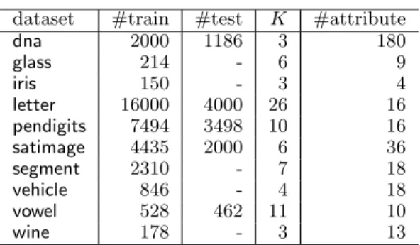
We tested AdaBoost.ERP experimentally on ten mul-ticlass benchmark problems (Table 1) from the UCI machine learning repository (Hettich et al., 1998) and the StatLog project (Michie et al., 1994). For problems with both training and test sets, experiments were run 100 times and the results were averaged. Otherwise, a 10-fold cross-validation was repeated 10 times for a total of 100 runs. When there was randomness in the learning algorithm and/or cross-validation was used, the standard error over 100 runs was also computed. For each run, the training part of the examples were linearly scaled to [−1,1], and then the test examples were adjusted accordingly.
We tried different ways to set the initial partitions and different schedules to repartition. In the results re-ported here, the initial partial partitions always con-tained two classes selected from all theKclasses, ran-domly (denoted byrand-2) or to maximize the corre-sponding Ut (denoted by max-2). We use a string of “L” and “R” to represent the schedule of base learn-ing and repartitionlearn-ing in a boostlearn-ing iteration. For ex-ample, “LRL” means that a base classifier was first learned on the two classes in the partial partition, then the partition was adjusted, and finally a new base clas-sifier was trained on the adjusted full partition.
Table 1. Multiclass problems dataset #train #test K #attribute
dna 2000 1186 3 180 glass 214 - 6 9 iris 150 - 3 4 letter 16000 4000 26 16 pendigits 7494 3498 10 16 satimage 4435 2000 6 36 segment 2310 - 7 18 vehicle 846 - 4 18 vowel 528 462 11 10 wine 178 - 3 13
We used four base learners of various degrees of com-plexity. The first one is the decision stump, also known as FindAttrTest(Schapire, 1997). The second one is the perceptron with a learning algorithm suitable
for boosting (Li, 2005). The third one is a binary
AdaBoost (Freund & Schapire, 1996) that aggregates up to 50 decision stumps. The last one is the soft-margin support vector machine with the perceptron kernel (SVM-perceptron) (Lin & Li, 2005).5
We compared our algorithm with AdaBoost.ECC with max-cut or rand-half. When the decision stump was used as the base learner, each algorithm was run for 500 iterations; for other more powerful base learners, the number of iterations was 200. However, for one ex-ception, theletterdata with 26 classes, we ran 1000 it-erations with the decision stump and 500 itit-erations
with other base learners. Note also that the exact
max-cutfor 26 classes is time-consuming so instead we used a simple greedy approximation for theletterdata
to approximately maximizeUtfor AdaBoost.ECC. We
also compared with one-vs-one and one-vs-all using the same base learners. For space consideration, we only list the lower test errors of these two algorithms. Table 2 presents the test errors with the decision stump as the base learner, the lowest errors in bold. With this simple base learner, one and one-vs-all got quite large errors since they are limited in the number of base classifiers. We can also see that most
of the time AdaBoost.ECC with max-cut was worse
than AdaBoost.ECC withrand-half. This verified our analysis that, when the base learner is not powerful enough, problems frommax-cutwould be too hard and the overall learning performance would instead be de-teriorated (see also Figure 4). With the help of reparti-tioning, AdaBoost.ERP achieved better test errors for most of the data sets, and for some cases it was sub-stantially better. For better illustration, we also show in Figure 4 the training cost and the test error curves for two large data sets, letterandpendigits. With the same number of base classifiers, AdaBoost.ERP almost always achieved a much lower training cost and a lower test error. More steps of the repartitioning and base learning further improved the learning, although the marginal improvement was small.
5
For the perceptron kernel, only the regularization pa-rameter C needs to be tuned. For problems with both training and test sets, a cross-validation with 30% of the training set kept for validation was repeated 10 times. The bestC∈˘
2−3,1,23,26,29¯
was then used in the full train-ing and testtrain-ing. The whole process was repeated 20 time. For problems with no test sets, the best results of the 10-fold cross-validation averaged over 10 times were reported. To support the weighted data, we scaleCfor each example proportional to its sample weight (Vapnik, 1999).
Table 2. Test errors (%) of multiclass algorithms with the decision stump as the base learner
one-vs-one AdaBoost.ECC AdaBoost.ERP (max-2) AdaBoost.ERP (rand-2)
dataset one-vs-all max-cut rand-half LRL LRLR LRL LRLR
dna 30.61 5.90 5.92±0.02 6.41 5.56 5.78±0.03 5.88±0.03 glass 34.10±1.11 27.43±0.95 26.67±0.92 26.05±0.85 25.57±0.89 25.29±0.85 25.62±0.85 iris 7.60±0.55 7.67±0.61 6.60±0.60 6.73±0.59 6.80±0.59 7.53±1.10 6.60±0.59 letter 39.42 32.79±0.19 22.00±0.04 21.05 17.73 18.52±0.03 17.84±0.02 pendigits 23.67 9.06 5.94±0.02 6.03 5.80 5.65±0.03 5.55±0.02 satimage 19.15 14.50 12.57±0.04 12.10 12.45 12.59±0.04 12.58±0.04 segment 12.24±0.21 3.28±0.12 1.94±0.09 2.07±0.09 1.97±0.09 1.90±0.09 1.95±0.09 vehicle 43.31±0.48 26.93±0.40 22.13±0.38 23.28±0.38 22.85±0.39 22.08±0.39 22.40±0.41 vowel 57.14 59.74 57.98±0.16 55.63 59.09 57.40±0.15 57.65±0.13 wine 15.33±0.71 2.00±0.32 3.17±0.39 2.33±0.36 2.72±0.39 2.83±0.37 2.78±0.37 0 200 400 600 800 1000 10−1 100 Number of iterations
Training cost (normalized)
AdaBoost.ECC (max−cut) AdaBoost.ECC (rand−half) AdaBoost.ERP (max−2, LRL) AdaBoost.ERP (rand−2, LRL) AdaBoost.ERP (rand−2, LRLR)
(a) cost on the letterdata
0 200 400 600 800 1000 15 20 25 30 35 40 45 50 55 60 Number of iterations Test error (%)
(b) test error on theletterdata
0 100 200 300 400 500
10−2
10−1 100
Number of iterations
Training cost (normalized)
AdaBoost.ECC (max−cut) AdaBoost.ECC (rand−half) AdaBoost.ERP (max−2, LRL) AdaBoost.ERP (rand−2, LRL) AdaBoost.ERP (rand−2, LRLR)
(c) cost on thependigitsdata
0 100 200 300 400 500 5 10 15 20 Number of iterations Test error (%)
(d) test error on thependigitsdata
Figure 4.Multiclass boosting with the decision stump (AdaBoost.ERP (max-2, LRLR) is very close to that withrand-2)
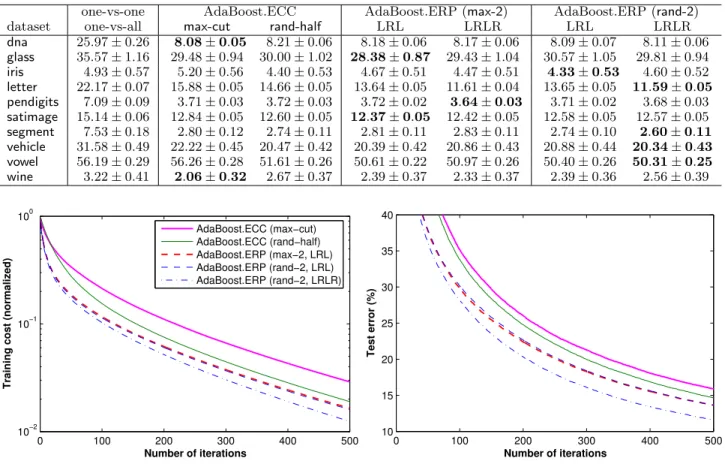
With the perceptron as a more powerful base learner, test errors on some data sets were greatly reduced (Ta-bles 3, with less number of iterations compared to that with the decision stump). Again repartitioning im-proved the learning performance on most of the data sets. Figure 5 shows the training cost and the test
error curves for the letter data set. Observations are similar to those of Figure 4, but the improvement was not as dramatic as with the decision stump.
The binary AdaBoost was the only weak learner with which one-vs-one actually had comparable or even
bet-Table 3. Test errors (%) of multiclass algorithms with the perceptron as the base learner
one-vs-one AdaBoost.ECC AdaBoost.ERP (max-2) AdaBoost.ERP (rand-2)
dataset one-vs-all max-cut rand-half LRL LRLR LRL LRLR
dna 25.97±0.26 8.08±0.05 8.21±0.06 8.18±0.06 8.17±0.06 8.09±0.07 8.11±0.06 glass 35.57±1.16 29.48±0.94 30.00±1.02 28.38±0.87 29.43±1.04 30.57±1.05 29.81±0.94 iris 4.93±0.57 5.20±0.56 4.40±0.53 4.67±0.51 4.47±0.51 4.33±0.53 4.60±0.52 letter 22.17±0.07 15.88±0.05 14.66±0.05 13.64±0.05 11.61±0.04 13.65±0.05 11.59±0.05 pendigits 7.09±0.09 3.71±0.03 3.72±0.03 3.72±0.02 3.64±0.03 3.71±0.02 3.68±0.03 satimage 15.14±0.06 12.84±0.05 12.60±0.05 12.37±0.05 12.42±0.05 12.58±0.05 12.57±0.05 segment 7.53±0.18 2.80±0.12 2.74±0.11 2.81±0.11 2.83±0.11 2.74±0.10 2.60±0.11 vehicle 31.58±0.49 22.22±0.45 20.47±0.42 20.39±0.42 20.86±0.43 20.88±0.44 20.34±0.43 vowel 56.19±0.29 56.26±0.28 51.61±0.26 50.61±0.22 50.97±0.26 50.40±0.26 50.31±0.25 wine 3.22±0.41 2.06±0.32 2.67±0.37 2.39±0.37 2.33±0.37 2.39±0.36 2.56±0.39 0 100 200 300 400 500 10−2 10−1 100 Number of iterations
Training cost (normalized)
AdaBoost.ECC (max−cut) AdaBoost.ECC (rand−half) AdaBoost.ERP (max−2, LRL) AdaBoost.ERP (rand−2, LRL) AdaBoost.ERP (rand−2, LRLR) 0 100 200 300 400 500 10 15 20 25 30 35 40 Number of iterations Test error (%)
Figure 5. Multiclass boosting with the perceptron on theletterdata
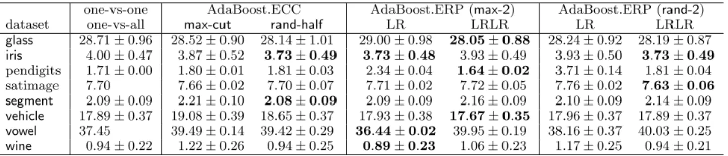
ter performance compared to the boosting algorithms. So we mark in Table 4 both the lowest errors among the boosting algorithms and the lowest errors among all the algorithms. Note that with this base learner, AdaBoost.ERP with only one base learning and one repartitioning (“LR”) was already comparable to Ada-Boost.ECC with base learning on the full training set. SVM-perceptron brought us the overall lowest test er-rors for most of the data sets (Table 5). Note that we do not have all the results for dnaandletter since parameter selection on an ensemble of SVMs is time-consuming. With this powerful base learner, all the multiclass algorithms performed comparably well, al-though AdaBoost.ERP was still better for some data sets. AdaBoost.ERP was also much faster compared to AdaBoost.ECC even though two SVMs may be learned in one iteration of AdaBoost.ERP, since the binary problems were usually easier.
5. Conclusion
We have proposed and tested AdaBoost.ERP, a new multiclass boosting algorithm with error-correcting
codes and repartitioning. The repartitioning is meant to find a better coding matrix according to the learning ability of the base learner. Our experimental results have shown that, compared with AdaBoost.ECC, one-vs-one, and one-vs-all, AdaBoost.ERP achieved the lowest training cost and test error on most of the real-world data sets we used. The improvement can be especially significant when the base learner is not very powerful. AdaBoost.ERP was also faster than Ada-Boost.ECC when working with SVM-perceptron. Simple algorithms like one-vs-one have their advan-tages. Compared to boosting algorithms, their train-ing time is usually much less, and the test error can be comparable or even lower when powerful base learners are used. The test time can also be substantially re-duced (Platt et al., 2000). Thus it is interesting to see how boosting algorithms can be further improved in these aspects.
Acknowledgments
The author thanks Yaser Abu-Mostafa, Alex Holub, and the anonymous reviewers for helpful comments.
Table 4. Test errors (%) with the AdaBoost that aggregates 50 decision stumps as the base learner
one-vs-one AdaBoost.ECC AdaBoost.ERP (max-2) AdaBoost.ERP (rand-2)
dataset one-vs-all max-cut rand-half LR LRLR LR LRLR
dna 6.32 7.93 7.30±0.03 7.50 6.75 7.48±0.05 7.17±0.04 glass 26.57±0.87 27.29±0.96 26.52±0.91 26.48±0.92 26.48±0.94 26.62±0.95 25.57±0.90 iris 6.00±0.60 6.40±0.58 7.00±0.57 5.67±0.59 6.20±0.59 79.33±0.75 9.13±1.47 letter 12.12 40.12±0.24 20.82±0.05 27.88 16.05 16.89±0.05 16.30±0.04 pendigits 4.92 8.81 5.37±0.02 4.00±0.01 5.69 5.55±0.08 5.12±0.02 satimage 12.55 14.60 13.87±0.04 14.75 13.65 12.74±0.05 13.67±0.04 segment 2.66±0.11 2.44±0.10 1.89±0.08 1.94±0.10 2.15±0.09 2.18±0.10 1.96±0.09 vehicle 24.66±0.41 24.60±0.47 22.82±0.45 26.01±0.43 23.32±0.44 22.80±0.43 23.05±0.44 vowel 46.10 56.93 56.64±0.14 50.33±0.03 57.14 51.35±0.23 56.21±0.14 wine 2.61±0.34 4.72±0.51 2.94±0.40 3.50±0.42 4.72±0.48 3.17±0.37 3.22±0.42 Table 5. Test errors (%) of multiclass algorithms with the SVM-perceptron as the base learner
one-vs-one AdaBoost.ECC AdaBoost.ERP (max-2) AdaBoost.ERP (rand-2)
dataset one-vs-all max-cut rand-half LR LRLR LR LRLR
glass 28.71±0.96 28.52±0.90 28.14±1.01 29.00±0.98 28.05±0.88 28.24±0.92 28.19±0.87 iris 4.00±0.47 3.87±0.52 3.73±0.49 3.73±0.48 3.93±0.49 3.93±0.50 3.73±0.49 pendigits 1.71±0.00 1.80±0.01 1.81±0.03 2.34±0.04 1.64±0.02 3.71±0.14 1.81±0.04 satimage 7.70 7.66±0.02 7.70±0.07 7.71±0.02 7.72±0.05 7.76±0.02 7.63±0.06 segment 2.09±0.09 2.21±0.10 2.08±0.09 2.09±0.09 2.16±0.09 2.10±0.09 2.14±0.09 vehicle 17.89±0.37 19.08±0.39 18.65±0.37 17.93±0.38 17.67±0.35 17.96±0.37 17.89±0.37 vowel 37.45 39.49±0.14 39.42±0.29 36.44±0.02 39.95±0.19 38.16±0.37 40.03±0.25 wine 0.94±0.22 1.22±0.26 0.94±0.25 0.89±0.23 1.06±0.23 1.17±0.25 0.94±0.21
This work was supported by the Caltech SISL Gradu-ate Fellowship.
References
Allwein, E. L., Schapire, R. E., & Singer, Y. (2000). Reducing multiclass to binary: A unifying approach for margin classifiers. Journal of Machine Learning Research,1, 113–141.
Dietterich, T. G., & Bakiri, G. (1995). Solving multi-class learning problems via error-correcting output codes.Journal of Artificial Intelligence Research,2, 263–286.
Freund, Y., & Schapire, R. E. (1996). Experiments
with a new boosting algorithm. Machine Learning:
Proceedings of the Thirteenth International Confer-ence (ICML ’96)(pp. 148–156). Morgan Kaufmann. Guruswami, V., & Sahai, A. (1999). Multiclass learn-ing, boostlearn-ing, and error-correcting codes. Proceed-ings of the Twelfth Annual Conference on Computa-tional Learning Theory(pp. 145–155). ACM Press. Hettich, S., Blake, C. L., & Merz, C. J. (1998). UCI
repository of machine learning databases.
Li, L. (2005). Perceptron learning with random
co-ordinate descent (Computer Science Technical Re-port CaltechCSTR:2005.006). California Institute of Technology, Pasadena, CA.
Lin, H.-T., & Li, L. (2005). Novel distance-based SVM kernels for infinite ensemble learning.Proceedings of the 12th International Conference on Neural Infor-mation Processing(pp. 761–766).
Mason, L., Baxter, J., Bartlett, P., & Frean, M. (2000). Functional gradient techniques for combining hy-potheses. In A. J. Smola, P. L. Bartlett, B. Sch¨olkopf
and D. Schuurmans (Eds.),Advances in large
mar-gin classifiers, chapter 12, 221–246. MIT Press. Michie, D., Spiegelhalter, D. J., & Taylor, C. C. (Eds.).
(1994). Machine learning, neural and statistical
classification. Ellis Horwood.
Platt, J. C., Cristianini, N., & Shawe-Taylor, J. (2000). Large margin DAGs for multiclass classification. Ad-vances in Neural Information Processing Systems 12 (pp. 547–553). MIT Press.
Schapire, R. E. (1997). Using output codes to boost
multiclass learning problems. Machine Learning:
Proceedings of the Fourteenth International Confer-ence (ICML ’97)(pp. 313–321). Morgan Kaufmann. Sun, Y., Todorovic, S., Li, J., & Wu, D. (2005). Unify-ing the error-correctUnify-ing and output-code AdaBoost
within the margin framework.ICML 2005:
Proceed-ings of the 22nd International Conference on Ma-chine Learning(pp. 872–879). Omnipress.
Vapnik, V. N. (1999).The nature of statistical learning theory. Springer-Verlag. 2nd edition.