HAL Id: tel-01551786
https://tel.archives-ouvertes.fr/tel-01551786
Submitted on 30 Jun 2017HAL is a multi-disciplinary open access archive for the deposit and dissemination of sci-entific research documents, whether they are pub-lished or not. The documents may come from
L’archive ouverte pluridisciplinaire HAL, est destinée au dépôt et à la diffusion de documents scientifiques de niveau recherche, publiés ou non, émanant des établissements d’enseignement et de
Machine Learning Strategies for Large-scale Taxonomies
Rohit Babbar
To cite this version:
Rohit Babbar. Machine Learning Strategies for Large-scale Taxonomies. Artificial Intelligence [cs.AI]. Université de Grenoble, 2014. English. �NNT : 2014GRENM064�. �tel-01551786�
TH `
ESE
Pour obtenir le grade de
DOCTEUR DE L’UNIVERSIT ´
E DE GRENOBLE
Sp ´ecialit ´e : Informatique Arr ˆet ´e minist ´erial : 7 ao ˆut, 2006
Pr ´esent ´ee par
Rohit Babbar
Th `ese dirig ´ee parEric Gaussier
et codirig ´ee parMassih-Reza Amini
pr ´epar ´ee au sein Laboratoire d’Informatique de Grenoble
et de Ecole Doctorale Math ´ematiques, Sciences et Technologies de l’Information, Informatique
Machine Learning Strategies for
Large-scale Taxonomies
Th `ese soutenue publiquement le17 Octobre, 2014, devant le jury compos ´e de :
Yann Guermeur
Professeur, Universit ´e de Lorraine, Rapporteur
Yiming Yang
Professeur, School of Computer Science of Carnegie Mellon University, Rapporteur
Thierry Arti `eres
Professeur, Universit ´e Pierre et Marie Curie, Paris, Examinateur
Bernhard Sch ¨olkopf
Director, Max Planck Institute for Intelligent Systems, T ¨ubingen, Examinateur
Denis Trystram
Professeur, Grenoble Institute of Technology, Examinateur
Eric Gaussier
Professeur, Laboratoire d’Informatique de Grenoble, Directeur de th `ese
A B S T R A C T
In the era of Big Data, we need efficient and scalable machine learning algo-rithms which can perform automatic classification of Tera-Bytes of data. In this thesis, we study the machine learning challenges for classification in large-scale taxonomies. These challenges include computational complexity of training and prediction and the performance on unseen data. In the first part of the the-sis, we study the underlying power-law distribution in large-scale taxonomies. This analysis then motivates the derivation of bounds on space complexity of hierarchical classifiers. Exploiting the study of this distribution further, we then design classification scheme which leads to better accuracy on large-scale power-law distributed categories. We also propose an efficient method for model-selection when training multi-class version of classifiers such as Support Vector Machine and Logistic Regression. Finally, we address another key model selection problem in large-scale classification concerning the choice between flat versus hierarchical classification from a learning theoretic aspect. The presented generalization error analysis provides an explanation to empirical findings in many recent studies in large-scale hierarchical classification. We further exploit the developed bounds to propose two methods for adapting the given taxonomy of categories to output taxonomies which yield better test accuracy when used in a top-down setup.
C O N T E N T S
1 introduction 1
1.1 Big Data and Large-scale Learning 1 1.2 Challenges in Large-scale Supervised
Learning 2
1.2.1 Cardinality of Training and Feature set sizes 3 1.2.2 Large number of Target Categories 3
1.2.3 Power-law behavior of Data 4
1.2.4 Exploiting Semantic Structure Among Categories 6 1.3 Contributions 7
1.4 Outline 9
2 state-of-the-art review 11 2.1 Flat Classification 12
2.1.1 Binary classification and One-vs-Rest 12 2.1.2 Crammer-Singer Multi-class SVM 14
2.1.3 Parallelizable Multinomial Logistic Regression 15 2.1.4 Trace-norm for large-scale learning 16
2.1.5 Other Approaches and Theoretical Studies 17 2.2 Hierarchical Classification 19
2.2.1 Pachinko-machine based deployment of classifiers 19 2.2.2 Tree-loss based optimzation 20
2.2.3 Recursive Regularization 21
2.2.4 Hierarchical Classification by Orthogonal Transfer 23
2.2.5 Other techniques and applications of hierarchical classification 24 2.3 Taxonomy Adaptation 24
2.3.1 Distribution Calibration 25 2.3.2 Hierarchy Flattening 26 2.4 Taxonomy Learning 27
2.4.1 Relaxed discriminative learning 27
2.4.2 Fast and balanced approach to taxonomy learning 28 2.5 Power-law in large-scale taxonomies 29
2.5.1 Training-time complexity 30 2.6 Conclusion 31
3 distribution of data in large-scale taxonomies 33 3.1 Introduction 33
3.2 Related Work 35
3.3 Power-law distribution in Large-scale Taxonomies 37 3.3.1 Yule’s model 38
3.3.2 Preferential attachment models for networks and trees 41 3.3.3 Model for hierarchical web taxonomies 42
3.3.4 Other interpretations 44 3.3.5 Limitations 45
3.3.6 Statistics per level in the hierarchy 45 3.4 Space Complexity Analysis 46
3.4.1 Relation between category size and number of features 46 3.4.2 Space Complexity of Large-Scale Classification 47
3.5 Conclusion 52
4 exploiting data-distribution for learning 55
4.1 Soft-thresholding for Classification in Power-law Distributed Categories 56 4.1.1 Power-law distribution 56
4.1.2 Related work and our contributions 58
4.1.3 Accuracy Bound on Power-law Distributed Categories 59 4.1.4 Soft-thresholding Algorithm for Higher Bound-value 60 4.1.5 Experimental Evaluation 63
4.1.6 Remarks 66
4.2 Efficient Model-selection in Big Data 67 4.2.1 Related Work 68
4.2.2 Accuracy Bound for Classification in Large Number of Categories 69 4.2.3 Using accuracy bound as alternative tok-fold cross-validation 70 4.2.4 Experimental Evaluation 72
4.2.5 Results 75 4.2.6 Remarks 76
4.3 Data-dependent Classifier Selection 76 4.3.1 Sample Complexity and LSHC 79 4.3.2 Experimental Setup 83
4.3.3 Results and Analysis 85 4.3.4 Remarks 86
4.4 Conclusion 86
5 flat versus hiearchical classification in large-scale taxonomies 89 5.1 Introduction 89
5.2 Related Work 92
5.3 Rademacher Complexity : A Review 94
5.4 Flat vs Hierarchical Classification : A learning theoretic View-point 95 5.4.1 A hierarchical Rademacher data-dependent bound 96
5.4.2 Lowering the bound by hierarchy pruning 99 5.5 Meta-learning based pruning strategy 102
5.5.1 Asymptotic approximation error bounds for Naive Bayes 102 5.5.2 Asymptotic approximation error bounds for Multinomial Logistic
Regression 105
5.5.3 A learning based node pruning strategy 108 5.6 Experimental Analysis 109
5.6.1 Flat versus Hierarchical classification 113 5.6.2 Effect of pruning 114
5.6.3 Effect of number of pruned nodes for meta-learning based pruning strategy 115
5.7 Conclusion 116
L I S T O F F I G U R E S
Figure1 Distribution of training instances among categories for Wikipedia subset from LSHTC 5
Figure2 Comparison of distribution of test instances in true dis-tribution and that induced by flat SVM classifier 6
Figure3 DMOZ and Wikipedia Taxonomies 7
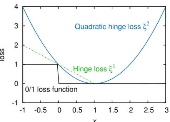
Figure4 Convex relaxations of 0-1loss in the form of Hinge and Squared hinge loss 13
Figure5 Spectrum of classification weight matrixWlearned on an Imagenet subset as shown in Harchaoui et al. [2012] 17
Figure6 Top-down deployment of SVM classifiers 20
Figure7 Top-level flattening of hierarchy 26
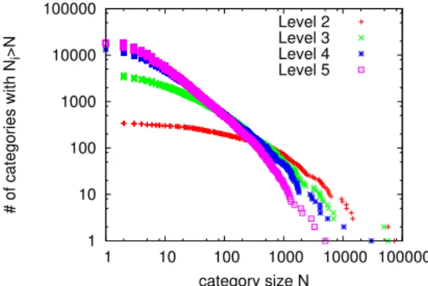
Figure8 Category size distribution for each level of the LSHTC2
-DMOZ dataset. 30
Figure9 DMOZ and Wikipedia Taxonomies 34
Figure10 Category size vs rank distribution for the LSHTC2-DMOZ
dataset. 37
Figure11 Indegree vs rank distribution for the LSHTC2-DMOZ
dataset. 38
Figure12 Number of categories at each level in the hierarchy of the LSHTC2-DMOZ database. 38
Figure13 Illustration of growth of taxonomy 41
Figure14 A website is assigned to existing categories with p(k) ∝ Nk. 43
Figure15 (ii): Growth in categories is equivalent to growth of the tree structure in terms of in-degrees. 43
Figure16 (iii): Growth in children categories. 43
Figure17 Model without and with shrinking categories. In the left figure, a child category inherits all the elements of its parent and takes its place in the size distribution. 44
Figure18 Category size distribution for each level of the LSHTC2
-DMOZ dataset. 45
Figure19 Number of features vs number of documents of each category. 46
Figure20 Heaps’ law: number of distinct words vs. number of words, and vs number of documents. 47
Figure21 Power-law variation for features in different levels for LSHTC2-a dataset, Y-axis represents the feature set size plotted against rank of the categories on X-axis 49
Figure22 Comparison of distribution of test instances for true dis-tribution and that induced by flat SVM classifier 57
Figure23 Comparison of distribution of test instances for proposed method and that induced by flat SVM classifier 64
Figure24 Distribution of training instances among categories for Wikipedia subset from LSHTC 67
Figure25 Variation (with λ) of cross-validation accuracy and the
derived bound 74
Figure26 Sample Taxonomy of Classes 77
Figure27 Top-down deployment of classifiers in uniform and hy-brid fashion 79
Figure28 Variation in ratio of feature set size to training sample
size 82
Figure29 Hybird Classifier deployment using Adaptive Selection 83
Figure30 Difference of SVM and NB accuracy 85
Figure31 DMOZ and Wikipedia Taxonomies 90
Figure32 The pruning procedure; the node in black is replaced by its children. 100
Figure33 Depiction of pruning procedure 108
Figure34 Distribution of data among classes 113
Figure35 Accuracy performance with respect to the number of pruned nodes for MNBon different test sets. 116
Figure36 Accuracy performance with respect to the number of pruned nodes forMLR(down) on different test sets. 117
L I S T O F TA B L E S
Table1 LSHTC and BioAsQ datasets and their properties 2
Table2 Summary of notation 40
Table3 Datasets for hierarchical classification with the proper-ties: Number of training/test examples, target classes and size of the feature space. 51
Table4 Model size (in GB) for flat and hierarchical models along with the corresponding values defined in Proposition 1. The symbol▽refers to the quantity K−b(KL−1) 52
Table5 LSHTC datasets and their properties 63
Table6 Comparison of Methods 65
Table7 Dataset description 72
Table8 Variation in accuracy with λparameter 75
Table9 Training Data Properties 84
Table10 Accuracy-Computational Complexity tradeoff 84
Table11 Dataset description 111
Table12 Comparison of Methods 112
1
I N T R O D U C T I O N
1
.
1
big data and large
-
scale learning
With an increasing amount of data from various sources such as web advertizing, social media and images, automatic classification of unseen data to one of tens of thousand target classes has caught the attention of the research community. This is due to the tremendous growth in data from various sources such as social networks, web-directories and digital encyclopedias. Some of the interesting facts which emphasize the need for effective automated organization of data are the following:
• Around one thousand new articles that are added everyday to english Wikipedia
• Approximately100hours of video is uploaded to Youtube every minute
• Close to20,000of scientific articles are added to PubMed1 every week
In order to maintain interpretability and to make these systems scalable, digital data are required to be classified among one of tens of thousands of target cate-gories. Directory Mozilla2, for instance, lists over 4million websites distributed
among close to 1million categories. In the more commonly used Wikipedia, which consists of over30 million pages, documents are typically assigned to multiple categories which are shown at the bottom of each page. The Medical Subject Heading hierarchy of the National Library of Medicine is another in-stance of a large-scale classification system in the domain of life sciences. In order to minimize the amount of human effort involved in such large-scale scenarios, there is a definite need to automate the process of classification of data into the target categories. To effectively address the computational barriers posed by theBig Data, the classical techniques of learning from data need to be adapted in order to tackle large-scale classification problems.
1 http://www.ncbi.nlm.nih.gov/pubmed
In the context of large-scale hierarchical classification (LSHC), open challenges like the Pascal Large Scale Hierarchical Text Classification (LSHTC) 3 and Imagenet Large Scale Visual Recognition Challenge (ILSVRC) 4 have been
organized. In the domain of life-sciences, the BioAsQ challenge 5 has been organized for classifying the medical abstracts. These challenges play an important role in evaluating the current state-of-the-art techniques for large-scale classification. Table1shows the statistics of the various datasets released as part of the LSHTC and BioAsQ challenge.
Dataset Training
instances
Categories Features Parameters (in GB) DMOZ-2010 128,710 12,294 381,580 4.3 DMOZ-2011 394,756 27,875 594,158 15.4 DMOZ-2012 383,408 11,947 348,548 3.8 SWiki-2011 456,886 36,504 346,299 11.7 LWiki-2013 2,817,603 325,056 1,617,899 489.7 BioAsQ-2013 10,876,004 26,563 444,085 10.9
Table1: LSHTC and BioAsQ datasets and their properties
In the next section, we highlight in detail the research challenges posed by classification problems for the datasets at the scale as shown in this table.
1
.
2
challenges in large
-
scale supervised arning
Most machine learning methods and algorithms have focused primarily on datasets which are of the order of the UCI datasets A. Asuncion [2007]. However, given the scale of modern datasets as demonstrated by LSHTC datasets, the nature of classification task is quite different as compared to that for smaller datasets such as UCI. Some of the interesting research problems posed for machine learning methods involving large-scale datasets are the following:
3 http://lshtc.iit.demokritos.gr/
4 http://www.image-net.org/challenges/LSVRC/2011/
1.2.1 Cardinality of Training and Feature set sizes
The number of training examples in modern large-scale learning problems are of the order of millions. This characteristic of the data poses significant computational challenges in the following ways :
• Scale of convex optimization problems: The intermediate convex
opti-mization problems involving minimizing convex surrogate losses such as Hinge loss and Logistic loss Zhang [2004b], Tewari and Bartlett [2007], Bartlett et al. [2006]are in high dimensional spaces. As a result, many off-the-shelf solvers such as LibSVM Chang and Lin [2011] run out of memory and hence cannot be applied directly. In its own right, this has led to the growth of new optimization-based techniques such as sequential dual method Keerthi et al. [2008] and trust-region based Newton method Lin et al. [2008] for large-scale learning.
• Hyper-parameter Tuning : Tuning the hyper-parameters such as the
regularizationλparameter in Support Vector Machines Hastie et al. [2004] by the standard technique of k-fold cross-validation can be extremely computationally intensive. As another instance, on the Wikipedia-2011
dataset from the LSHTC challenge which has approximately0.5million training documents among36,000 categories, 5-fold cross-validation to learn the parameter λwill take around one month on a single quad-core machine with standard hardware.
1.2.2 Large number of Target Categories
Learning with large number of target categories poses a relatively new challenge in machine learning as compared to large-scale learning for binary classification or classification with few tens of categories. Large-scale learning involving classification among fewer categories has been well understood theoretically Bottou and Bousquet [2008] and also stochastic version SVM solvers such as Pegasos Shalev-Shwartz et al. [2011] are available. However, learning with tens of thousand target categories involves:
• Billions of parameters to learn : Large-scale learning involving large
number of target categories requires to learn one high dimensional weight vector for each category. For instance, for one of the LSHTC datasets, having 12,294categories in a feature set of size347,256 one needs to learn 12, 294×347, 256 =4.2billion parameters. In this context, the recent study by Gopal and Yang [2013a] presents a technique to learn Regularized Logistic Regression classifier by replacing the Logistic loss by an upper bound which can be easily parallelized.
• Class imbalance: One-vs-Rest framework, as studied in Rifkin and Klau-tau [2004], Allwein et al. [2001] and implemented in most modern solvers such as Liblinear Fan et al. [2008], is one of the standard methods to handle large number of categories. However, when dealing with large number of target categories makes the individual binary classification problem highly imbalanced and hence makes learning effective decision boundaries further difficult. Due to the high-dimensionality of the clas-sification problems, conventional methods for handling class-imbalance such as those proposed in Chawla et al. [2011], Tang et al. [2009b] are not effective in large-scale problems.
• Complexity of Inference : For large number of target categories, the
inference time becomes significantly important. For instance, to classify a test instance among K categories under the One-vs-Rest framework, one needs to evaluateO(K) classifiers Harchaoui et al. [2012], Perronnin et al. [2012]. This could be significantly high for large-scale classification problems involving tens of thousand categories. Many recent works such as Bengio et al. [2010], Gao and Koller [2011], Deng et al. [2011], Yang and Tsang [2012] have focused on learning a tree-based taxonomy of categories which aim at reducing the complexity of inference toO(lg(K)).
• Universal consistency: Another short-coming of the easily parallelizable
One-vs-Rest framework is that it does not satisfy universal consistency
property Tewari and Bartlett [2007]. On the other hand, the multi-class SVM proposed in Crammer and Singer [2002] enjoys good theoretical guarantees but is not separable into binary problems and hence not directly parallelizable.
1.2.3 Power-law behavior of Data
As shown in Figure1for the distribution of Wikipedia dataset from the LSHTC challenges, the distribution of data among categories follows power-law distri-bution. It has also been studied in the work of Liu et al. [2005] for large-scale web directories such as DMOZ and Yahoo! directory. Formally, let Nr denote
the size of ther-th ranked category (in terms of number of documents), then :
Nr = N1r−β (1.2.1) where N1 represents the size of the1-st ranked category and β > 0 denotes
the exponent of the power law distribution. As a result, a large fraction of categories consist of very few documents in them. For instance, as discussed in Gopal and Yang [2013b],76% of the categories in the Yahoo! directory have less than5documents in them and these are commonly referred to asrare categories. Another interpretation of this behavior is that the average number of documents
1 10 100 1000 10000 1 10 100 1000 10000 100000 Number of Documents Rank of Category Distribution of Data
Figure1: Distribution of456,866training instances (for a Wikipedia subset from LSHTC) among36,000 categories in the training data, with X-axis rep-resenting the rank (by number of documents) of categories and Y-axis the number of documents in those categories. Approximately 15,000
of the 36,000 categories have ≤5 documents, with 4,000 categories having just 1document in the training set.
per category decrease as the number of categories grow. This property of dataset leads to following problems in being to learn good classifiers:
• Due to insufficient data, it is difficult to learn good decision boundaries for rare categories.
• The class-imbalance problem is further aggravated in such power-law category systems.
As a result, a test instance which actually belongs to one of the rare categories is assigned to a bigger category. On one hand, this leads to high False Positive rate for bigger categories, and on the other hand, rare categories are lost in the classification process. This is shown for one of the datasets in Figure 2. For the distribution induced by the SVM classifier, observations in Figure 2which demonstrate the high False-positive rate for large categories and inability to detect rare categories in such distributions are :
• On the left side of the plot, the graph for the distribution induced by the SVM classifier starts higher and remains higher as compared to true distribution, but drops much sharply on the right part, and
• Comparing the tails of the distributions on the right side of the plot, the true distribution has a fatter tail as compared to the induced distribution, i.e., it has many more categories of1or2 documents as compared to the distribution induced by the SVM classifier.
1 10 100 1 10 100 1000 Number of Documents Rank of Category True distribution Distribution induced by a flat SVM classifier
Figure2: Comparison of distribution of test instances among categories in the true distribution and in the distribution induced by a flat SVM classifier; the X-axis represents the rank of categories (by number of documents) and Y-axis the number of documents in those categories. Categories with same number of documents effectively have same rank.
1.2.4 Exploiting Semantic Structure Among Categories
Typically, categories in large-scale systems have an inherent semantic structure among themselves. For instance, DMOZ is in the form of a rooted tree where a traversal of path from root-to-leaf depicts transformation of semantics from generalization to specialization. More generally parent-child relationship can exist in the form of directed acyclic graphs, as is found in the taxonomies such as Wikipedia. The tree and DAG relationship among categories is illustrated for DMOZ and Wikipedia taxonomies in Figure3.
Given the taxonomy structure, various approaches such as Gopal and Yang [2013b], Cai and Hofmann [2004], Dekel [2009] have been proposed which exploit this additional information differently. The taxonomy information among categories can mitigate the data-imbalance problem Babbar et al. [2013a] particularly in large-scale power-law distributed categories. Furthermore, one needs to evaluate onlyO(lg(K)) classifiers in tree-based classifiers, also it has been shown in the work of Liu et al. [2005] that the training time complexity of hierarchical classification is lower than that for flat classification.
However, the usage of taxonomy may have some undesirable impact on the classification performance of the top-down cascade, such as:
• Propagation Error: Using the top-down cascade of classifiers deployed
top-Root
Arts
Arts SportsSports
Movies Video Tennis Soccer
Players Fun
Arts
Theater Music
Drama Opera Pop Rock
Figure3: DMOZ and Wikipedia Taxonomies
levels towards the leaves. This cause of error is significant since the top-level categories are quite generic in nature and hence considerable overlap among them in feature space. For instance, theSportsandEntertainment
nodes in Yahoo! directory are likely to a have a high degree of common vocabulary between them. The application of Refined Expertsas studied in the work by Bennett and Nguyen [2009] aims to handle the propagation error in an effective manner.
• Noisy TaxonomiesThe taxonomy structure given a-priori as part of the
training data may not be best suited to yield high classification accuracy due to the following reasons:
1. Large-scale web taxonomies are designed with an intent of better user-experience and navigability, and not for the goal of classification.
2. Taxonomy design is subject to certain degree of arbitrariness based on personal choices and preferences of the editors.
3. The large-scale nature of such taxonomies poses difficulties in manu-ally designing good taxonomies for classification.
In the recent work by Dekel [2009] on relatively smaller taxonomies, the impact of arbitrariness on loss-function design is minimized by appropri-ately calibrating the edge distance between the true and predicted class. In similar spirit of taxonomy adaptation, approaches based on flattening the hierarchy such as Malik [2009], Wang and Lu [2010], have been pro-posed in LSHTC for large-scale settings which lead to improvement in classification accuracy as compared to using the original hierarchy.
1
.
3
contributions
In machine learning, a significant part of effort from a pedagogical view-point Sch ¨olkopf and Smola [2002], Bishop et al., Devroye [1996], Hastie et al. [2001] and also from the attempt to develop new methods towards addressing research challenges in machine learning Koller and Sahami [1997], McCallum et al. [1998],
Blei et al. [2003], McAllester [1998], Bousquet and Elisseeff [2002] have focused on relatively smaller sized datasets. In the light of the availability of Big data and the need to separate useful information from noise, the challenges posed by large-scale classification particularly in the presence of large number of target categories need to be addressed effectively. As discussed in the previous section, most naturally occurring large-scale datasets exhibit fit to power-law distribution and also have semantic structure among the target categories. In this direction, we attempt to address some of the theoretical aspects of this research challenge as well as also from the view-point of developing new methods for classification in large-scale taxonomies. Specifically, our contributions in this thesis are the following:
• We first study the distribution of data in large-scale taxonomies and vari-ous generative models which give rise to the fit to power-law distribution of documents among categories in large-scale taxonomies. We refer to the famous model by Yule Yule [1925] which is governed by the assumption that a new elements joins an existing category with the probability that is proportional to its current size. In the context of large-scale taxonomies, we also study other models such as those based on Preferential attach-ment Barab´asi and Albert [1999]. We complete our analysis of power-law behavior in large-scale taxonomies by deriving an analytical form for the upper bound of space complexity of hierarchical classification technique and provide a comparison to space complexity of flat classification. This work has been published in the Special Information Group on knowledge Discovery and Data Mining (SIGKDD) Explorations Journal,2014.
• Secondly, we exploit the distribution of data in large-scale category sys-tems to address the three challenges for classification, (i) classification accuracy, (ii) training time via model selection and hyper-parameter tun-ing, and (iii) prediction time. Addressing the problem depicted in Figure
2 which is faced by most state-of-the-art methods, we propose a sim-ple but non-trivial upper bound on the accuracy of a classifier which classifies instances among tens of thousand power-law distributed cate-gories. Our soft-thresholding based method for ranking target categories by their posterior probabilities is published in Special Information Group on Information Retrieval (SIGIR) 2014 Babbar et al. [2014]. Exploiting the accuracy upper bound further, we also demonstrate efficient method for model-selection as an alternative to computationally expensivek-fold cross-validation. Using the sample complexity bounds for discriminative and generative classifiers as derived in Ng and Jordan [2001], we also propose a method to combine Support Vector Machine and Naive Bayes classifiers in a top-down cascade which leads to faster training and predic-tion in large-scale hierarchical classificapredic-tion. This work Babbar et al. [2012]
and its variant Partalas et al. [2012] were published in Conference on Information and Knowledge Management (CIKM)2012, and International Conference on Neural Information Processing (ICONIP)2012 respectively.
• Lastly, we address the problem of flat versus hierarchical classification in large-scale taxonomies from a learning theoretic point of view. The goal in this problem is to learn from the training data to choose one of strategies, (i) use flat classification, i.e., ignore the given taxonomy structure alto-gether, or (ii) perform hierarchical classification with classifiers deployed in a top-down cascade. This research challenge, even though fundamental to the nature of classification problem in large-scale taxonomies, has not been addressed earlier from a learning-theoretic aspect. To our knowledge, our work Babbar et al. [2013a] in Neural Information Systems (NIPS)2013, was the first such attempt towards this problem wherein we developed Rademacher complexity based generalization error bounds to study this problem. In order to handle the noisy taxonomies, we further exploit the developed bounds for designing techniques using which the given can be adapted to learn a new taxonomy which leads to better classification accuracy. This can also be viewed as synchronization of two parts of the training data, (i) in the form of input, output pairshx,yi, and (ii) as given by the taxonomy. This work was published in International Conference on Neural Information Processing (ICONIP)2013. The work presented in this chapter is currently under revision after first round of reviews from Journal of Machine Learning Research (JMLR).
1
.
4
outline
The brief outline of the this thesis is as follows:
• In Chapter2, we review the current state-of-the-art for large-scale super-vised classification for flat and hierarchical classification. Even though, our focus is primarily on mono-label classification throughout the thesis, we also briefly mention some of the multi-label approaches for large-scale classification.
• We present in Chapter3, various generative models which lead to the fit to power-law distribution of documents among categories in large-scale taxonomies. We also present an analytical study of the space complexity of hierarchical classification.
• In Chapter 4, we also derive non-trivial upper bound on the accuracy of a classifier which is particularly useful in large-scale power-law distributed
categories. Based on this upper-bound, we propose techniques for better classification accuracy and efficient model selection.
• In Chapter5, we present the learning theoretic bounds for top-down hier-archical classification and address the flat versus hierhier-archical classification problem in large-scale taxonomies. We also propose two methods for taxonomy adaptation by hierarchy pruning which is shown to yield better classification accuracy than the hierarchy of classes given a-priori.
2
S TAT E - O F - T H E - A R T R E V I E W
Classification of data into large-number of categories has assumed considerable significance over the last few years. This is due to considerable growth in data from various sources such as social media, commercial products and descrip-tions, images data from uploaded photos and videos, and from collaborative encyclopedias. For instance, enterprises such as Amazon and ebay have product hierarchies which are aimed at providing easy access to customers for searching the desired product and also other products which are closely related to itself. Furthermore, motivated by the challenge of fine-grained classification in the context of images, classification into large number of categories has become quite important.
As a result, the process of automatic classification is no longer restricted to small scale datasets with two or few tens of labels. In view of emerging commercial interests in large-scale problems and also public availability of such datasets, recent research interest in machine learning for tens of thousand target categories has increased considerably. This is also evident from large number of scientific publications in large-scale learning and big data every year which address various aspects of large-scale learning. Furthermore, big data has been the theme of many conferences and workshops in the recent years.
It is important to note that by large-scale learning we refer to large-number of target categories and focus on classification challenges arising out of such machine learning setting. By large-scale learning, we do not imply problem settings with binary classification problem such as when spam versus non-spam classification for a large corpus is performed. Even though classification for binary problem or with few tens of target categories on large datasets are interesting and have been studied (from the point of view of stochastic training) theoretically (Bottou and Bousquet [2008], Zhang [2004a]) and empirically (Shalev-Shwartz et al. [2011]).
Going beyond the classical problem in machine learning of designing a classifier with low generalization error, other metrics of evaluation such as prediction time, training time, and space complexity of the model become important in order the assess the quality of a classifier. The immediate approach to handle large number of categories is to consider them as many independent binary classification problems as the number of target categories, which is also referred
to as One-versus-Rest as discussed primarily in Rifkin and Klautau [2004], Allwein et al. [2001]. For SVM classifier, the method proposed by Weston [1998] to handle multi-class problems is by adding constraints for every category and thereby the number of constraints grow quadratically with number of target categories. Another approach for handling multi-class problems which is based on the generalized notion of margin for multi-class problems is proposed in Crammer and Singer [2002].
However, these multi-class approaches have prediction time which is linear in the of number of categories, i.e.,O(K) for K categories. For large number of target categories, in the range of tens of thousand, it is desired to have prediction time which is sublinear in the number of categories. Typically, for large number of categories, there exists a semantic structure among categories in the form of rooted tree or a directed cyclic graph. This can be viewed in the form of parent-child relationship which also depicts a transition from general categories to special categories when one traverses the path from root towards the leaves. In the light of the inherent existence of the semantic structure among categories, there has been significant research focus on hierarchical classification systems. In the next sections, we discuss the state-of-the-art methods for large-scale learning. Since flat classification is a special case of hierarchical classification in which case the taxonomy structure is ignored, we give below the more general formulation in terms of setup for hierarchical classification.
2
.
1
flat classification
Flat approaches to large-scale learning ignore the hierarchical structure among the categories. This makes them simpler to interpret and implement. However, these approaches may suffer from data-imbalance problem particularly in the presence of power-law distributed category systems.
2.1.1 Binary classification and One-vs-Rest
Most recent studies have focused on Support Vector Machines (SVM) and Logistic Regression (LR) for large-scale learning. These discriminative learning algorithms minimize a combination of empirical error and model complexity. The template of the objective function which is minimized is of the following form:
ˆ
w =arg min
w Remp(w) +λ Reg(w) (2.1.1) where Reg(w) is the regularization term to avoid complex models andRemp(.)
-1 0 1 2 3 4 -1 -0.5 0 0.5 1 1.5 2 2.5 3 loss x
Quadratic hinge loss ξ2
Hinge loss ξ1
0/1 loss function
Figure4: Convex relaxations of0-1loss in the form of Hinge and Squared hinge loss
In binary classification, the training set is of the form (xi,yi),i =1 . . .m,yi ∈
{−1,+1}. For SVM classifier, the 0-1 loss Remp(.) is replaced by its convex
surrogate called the hinge-loss which is given by (max(0, 1−yiwTxi)). For Logistic Regression Remp(.), the convex surrogate is based on logistic loss
(log(1+exp(−yiwTxi))). Reg(w)is typically of the form 12wTw, unless sparse solution is desired in which case it is replaced by|w|. The hyper-parameter λ
controls the trade-off between the empirical error and regularization term. More specifically, the optimization problem for learning binary L2-regularized, L1-loss SVM classifier is given by
min w λ 2||w|| 2+
∑
m i=1 (max(0, 1−yiwTxi))On similar lines, the L2-regularized, L2-loss SVM classifier min w λ 2||w|| 2+
∑
m i=1 (max(0, 1−yiwTxi))2The L1-loss and L2-loss relaxations are shown in Figure2.1.1. The L2-regularized, Logistic Regression classifier is given by
min w λ 2||w|| 2+
∑
m i=1 log(1+exp(−yiwTxi))To handle multi-class problems under the One-vs-Rest framework, one binary classifier which is parameterized by the weight vector wk is learnt for each
of the K target categories. The training data is transformed K times for the construction of each binary problem such that while learningwk the training instances which belong to category kare labeled +1 and all the other training
instances are labeled−1. At inference time, to estimate the target category of instancex, the predicted category is the one which satisfies arg maxkwTkx. This
approach has the following salient features:
• It is simple to interpret and more importantly, easily parallelizable which is a desirable property for training classifiers in settings with large number of target categories.
• It has been shown in the work of Rifkin and Klautau [2004], that when the binary classifiers are properly calibrated, the One-vs-Rest classifier can perform at par with other approaches such as One-versus-One and approaches based on Error Correcting Output Codes (Dietterich and Bakiri [1995]).
• A major drawback One-vs-Rest framework is that it does not satisfy
universal consistency property Tewari and Bartlett [2007] and hence does not enjoy strong theoretical guarantees.
2.1.2 Crammer-Singer Multi-class SVM
The approach studied in Crammer and Singer [2002] proposed a more natural way to handle to multi-class problem instead of considering them as indepen-dent binary problems. For given training data in the form of instance-label pairs (xi,yi),i =1 . . .m,yi ∈ {1 . . .K}, the formulation of the optimization problem under this framework is given by
min wk,ξi|| wk||2+C m
∑
i=1 ξiThe constraints for the above optimization problem are given by,∀i =1 . . .m
wTyixi−wTkxi ≥1−eik−ξi, and ξi ≥0 where eki = 1 if yi =k 0 otherwise
The decision function is given by
arg max
k=1...Kw T
The primal optimization problem as given above is typically solved from its dual formulation. The dual is given by the following
min α 1 2∑Kk=1||wk||2+∑im=1∑Kk=1ekiαki subject to ∑Kk=1αki =0, ∀i =1 . . .m αki ≤Ckyi∀i =1 . . .m,∀k =1 . . .K (2.1.2) where wk = m
∑
i=1 αikxi∀k, α= [α11. . .α1K, . . . ,α1m. . .αKm]T and Cyki = 0 if yi 6=k C otherwiseSequential dual method for solving the dual optimization problem in (mc-svm-dual-chap2) was proposed in Keerthi et al. [2008] for handling large-scale problems.
Unlike the one-vs-rest framework of handling multi-class problems, this formu-lation has strong theoretical guarantees such as universal consistency Tewari and Bartlett [2007], Zhang [2004b], Bartlett et al. [2006]. However, it suffers from two major disadvantages in the context of large-scale learning :
• Since it learns the parameterswk simultaneously for each target category, it is not inherently parallelizable, and hence may lead to extremely high training time. In a typical large-scale setting, since the dimensionality of eachwk is of the order of hundreds of thousand, and for a classification problem involving few tens of thousand categories, the total number of parameters are in the range of billions. Therefore, being able to parallelize the training procedure is highly desirable property.
• Furthermore, the memory requirements of this method are quite high as the tasks cannot be split across categories.
2.1.3 Parallelizable Multinomial Logistic Regression
To handle the drawbacks mentioned for the multi-class SVM in the formulation proposed by Crammer-Singer, the recent study in Gopal and Yang [2013a] proposes a method to parallelize the optimization of the objective function. For regularized multinomial logistic regression, the probability for instance x to belong to category kis given by
P(y=k|x) = exp(w
T kx)
∑Kk′=1exp(wTk′x)
LetW ={w1, . . . ,wK} denote the matrix of weight vectors, then the training
objective in this framework is given by
min W λ 2 K
∑
k=1 ||wk||2− K∑
k=1 N∑
i=1 ekiwTkxi+ N∑
i=1 log( K∑
k′=1 exp(wTk′x)) (2.1.3) As such the objective function given by the above equation is not parallelizable due to the coupling of all the class-level parameters together inside a log-sum-exp function. The authors use the concavity of the log-function to replace the objective in2.1.3by a parallelizable version. The log concavity bound is given bylog(γ) ≤aγ−log(a)−1, ∀γ,a >0
Using the above bound and introducing parametersaifor each training instance, the log-partition function for instance iis bounded as follows :
log( K
∑
k=1 exp(wTkxi)) ≤ai K∑
k=1 exp(wTkxi)−log(ai)−1From the above substitution and denoting byathe vector of ai,i=1 . . .m, the new objective function is given by
min W,a λ 2 K
∑
k=1 ||wk||2+ N∑
i=1 " − K∑
k=1 eikwTkxi+ai K∑
k=1 exp(wTkxi)−log(ai)−1 # (2.1.4) The above objective is parallelizable, even though non-convex. However, the authors shows that the new obejctive function in Equation 2.1.4 has many desirable properties such that it can be exploited to obtain the solution to the original ojective function in Equation2.1.3.2.1.4 Trace-norm for large-scale learning
Another important insight for large-scale classification in the context of image data has been done in Harchaoui et al. [2012], wherein the authors perform singular value decomposition on the matrix of weight vectors W and show that it has a rank which is much lower thanK. Motivated by this observation, they propose a learning objective which captures the low-rank embedding of the target categories. This is achieved by adding a low-rank enforcing penalty in the form of trace norm regularization to the Frobenius norm penalty. The learning objective considered in this work is of the form
Figure5: Spectrum of classification weight matrixWlearned on an Imagenet subset as shown in Harchaoui et al. [2012]
min
W λ1rank(W) +λ2||W||
2+R
m(W) (2.1.5)
where Rm(W) denotes the empirical risk
Rm(W) = 1 m m
∑
i=1 L(W;xi,yi)and the authors take multi-class logistic loss as the loss function to compute the empirical loss which has the following form
L(W;x,y) =log(1+
∑
k∈1...K/y
exp{wTkx−wTyx})
Since the objective function in2.1.5is non-smooth and non-convex, it is relaxed by replacing the rank(W) by its tightest convex surrogate i.e., the trace norm. The new objective function is given by
min
W λ1||W||σ,1+λ2||W||
2+R
m(W) (2.1.6)
where||W||σ,1 denotes the trace-norm ofW. The objective function in the above equation is convex but is non-differentiable due to the low-rank enforcing penalty. The authors demonstrate the similarity of this objecitve to sparse logistic regression for binary problems Hastie et al. [2001].
2.1.5 Other Approaches and Theoretical Studies
The work in Perronnin et al. [2012] is based on using One-versus-Rest classifier for large-scale image data from ILSVRC challange. They authors propose
some important recommendations for using One-vs-Rest strategy for image classification to achieve state-of-the-art performance using dense Fisher Vector representation of images S´anchez et al. [2013], Perronnin and Dance [2007]. The proposed recommendations include:
• Learning with stochastic gradient descent is well suited for large-scale datasets
• Early stopping can be used as an effective mechanism to achieve regular-ization
• A small-enough step-size w.r.t. the learning rate is sufficient for good performance
In the recent study by Weston et al. [2013], the authors propose a label par-titioning technique for sub-linear ranking involving large-number of labels. Another quite recent study for large-scale classification have been studied in the work of Gupta et al. [2014], wherein the authors propose to approximate the expected error with a different empirical loss called theempirical class-confusion loss. For the large-scale online training, they show that an online empirical class-confusion loss can be implemented for stochastic gradient descent by ignoring stochastic gradients corresponding to a repeated confusion between classes.
From a learning theoretic view-point, the work in Daniely et al. [2012] compares various multi-class approaches including multi-class SVM, vs-Rest, One-vs-One and tree-based classifiers Beygelzimer et al.. Some of the important findings of this study are the following:
• The estimation errors of One-vs-Rest, multi-class SVM, and tree-based classifiers are approximately close to each other,
• The authors prove that the hypothesis class of multi-class SVM essentially contains the hypothesis classes of both One-vs-Rest and tree-based clas-sifiers. Furthermore, these inclusions are strict and since the estimation errors of these three methods are roughly the same, it follows that the multi-class SVM method dominates both One-vs-Rest and tree-based classifiers in terms of achievable prediction performance, and
• They also show that the hypothesis class of One-vs-One essentially con-tains the hypothesis class of multi-class SVM, and that there can be a substantial gap in the containment.
The work in Guermeur [2007] also provides important theoretical insight into the VC-theory for class classification. In the context of large-scale multi-label classification various approaches such as Agrawal et al. [2013], Yu et al. [2013], Hariharan et al. [2010], Cisse et al. [2013].
2
.
2
hierarchical classification
In hierarchical classification, in addition to the input-output pairs, we are also given the taxonomy of classes which represents the underlying semantic structure. Formally, we use the following setup for understanding hierarchical classification and the approaches proposed to handle such problems.
Let X ⊆ Rd be the input space and let V be a finite set of class labels. We
further assume that examples are pairs (x,v) drawn according to a fixed but unknown distribution D overX ×V. In the case of hierarchical classification, the hierarchy of classes H = (V,E) is defined in the form of a rooted tree, with a root ⊥and a parent relationship π : V\ {⊥} → V where π(v) is the parent of node v ∈ V\ {⊥}, and E denotes the set of edges with parent to child orientation. For each node v ∈ V\ {⊥}, we further define the set of its sisters S(v) = {v′ ∈ V\ {⊥};v =6 v′∧π(v) = π(v′)} and its daughters
D(v) = {v′ ∈ V\ {⊥};π(v′) = v}. The nodes at the intermediary levels of the hierarchy define general class labels while the specialized nodes at the leaf level, denoted by Y ={y ∈ V : ∄v ∈ V,(y,v) ∈ E} ⊂V, constitute the set of target classes. Finally for each class y in Y we define the set of its ancestors
P(y) defined as P(y) = {vy1, . . . ,vyk y;v y 1 =π(y)∧ ∀l ∈ {1, . . . ,ky−1},v y l+1 =π(v y l)∧π(v y ky) =⊥}
Given a new test instance x, the goal is to predict the class yb. In top-down hierarchical classification, the classifier (such as SVM) is learnt at every decision node in the tree as is shown in Figure 2.2.1. The various state-of-the-art methods differ in the way they learn the classifier at each node. In the case of flat classification, the hierarchy His ignored,Y =V, and the problem reduces to the classical supervised multi-class classification problem.
2.2.1 Pachinko-machine based deployment of classifiers
In Pachinko-machine based top-down deployment of classifiers the decisions are made at each level of the hierarchy. This method selects the best class at each level of the hierarchy and iteratively proceeds down the hierarchy until a leaf node is reached. This is typically done by making a sequence of predictions iteratively in a top-down fashion starting from the root . At each non-leaf node
v ∈V, a score fc(x) ∈ Ris computed for each daughter c ∈D(v)and the child
b
c with the maximum score is predicted i.e. cb=arg maxc:(v,c)∈E fc(x).
For SVM classifier, fc(x) is modeled as a linear classifier such that fc(x) = wTcx.
Root
SVM SVMSVM
SVM SVM
SVM SVM
SVM SVM
Figure6: Top-down deployment of SVM classifiers
classifier for node v, the following optimization problem is solved for each daughterc ofv min wc,ξ λ 2||wc|| 2+
∑
mv i=1 ξ2(i,c)The indices i above are such that ∀i, 1 ≤ i ≤ mv,yi ∈ Lv, were Lv denotes
the set of leaves in the subtree rooted at node v and mv denotes the number
of training examples for which the root-to-leaf path passes through the node
v. Furthermore, if yi ∈ Lc and (v,c) ∈ E, then the constraints for the above
optimization problem are given by,∀i
wtcxi ≥1−ξ(i,c), and ξ(i,c) ≥0
This method has the advantage that it is faster to train and is very natually parallelizable owing to the independence of optimization problems at each node in the taxonomy. Furthermore, due to the tree-nature of the problem, the number of predictors that one needs to evaluate is logarithmic in the number of target categories. This method is shown to yield competetive performance on large-scale datasets as shown in the work of Liu et al. [2005], Dumais and Chen [2000]. However, many variants of this methods have been proposed recently.
2.2.2 Tree-loss based optimzation
In the recent work of Bengio et al. [2010], the authors observe that in a hierar-chical setup, the final prediction can be wrong due to mis-classification atany
node in the root to leaf path. This is unlike the Panchinko machine model in which each mis-classification at every node is accounted individually. With this insight as the motivation, they propose a tree-loss based optimization wherein the slack variable is shared acorss all nodes along each of the root to leaf path in the tree.
Denoting by bj(x) as the index of the best node (w.r.t. to the decision function) in the hierarchy at depth j Specifically, the loss function, calledtree loss, on the training data is given by
Remp(ftree) = 1 m m
∑
i=1 max j∈B(x)I(yi ∈ lj)where B(x) = {b1(x). . .bD(x)(x)} and D(x) denotes the depth in the tree for final prediction of instance x. Assuming that internal nodes of the tree are indexed by jandlj denotes the set of leaves under the sub-tree rooted at node j. Replacing the0-1loss function in the form of indicator function and adding the2-norm regularizer, the optimization objective is given by
|V|
∑
j=1 γ||wj||2+ 1 m m∑
i=1 ξij ! (2.2.1) such that ∀i,j Cj(yi)fj(xi) ≥1−ξij ξij ≥0whereCj(yi) = 1 if yi ∈ lj and -1otherwise.
To take into account the tree loss, the above optimization as given Equation
2.2.1 is modified by introducing a slack variable which is shared across all the decision nodes for a given training instance. This leads to the following tree-loss based optimization objective
γ |V|
∑
j=1 ||wj||2+ 1 m m∑
i=1 ξi (2.2.2) such that fr(xi) ≥ fs(xi) +1−ξi,∀r,s: yi ∈ lr∧yi ∈/ ls∧(∃p: (p,r) ∈ E∧(p,s)∧E) (2.2.3) ξi ≥0,∀i =1 . . .m (2.2.4) 2.2.3 Recursive RegularizationIn this recently proposed strategy Gopal and Yang [2013b], the hierarchy structure is incorporated into the optimization problem in the form a regularizer. In the hierarchical approaches, the weight vector is required to be learnt at each node of the hierarchy tree. Therefore, let the matrix W be such that its columns represent the weight vectors at each of the decision nodes, i.e.,
W = {wv,v ∈ V}. The regularization term for the optimization problem at
to that of its parent node. The framework is proposed for SVM and Logistic Regression classifier, and for SVM is given by the following:
HR-SVM min W v
∑
∈V 1 2||wv−wπ(v)|| 2+C∑
v∈Y m∑
i=1 (1−Cv(yi)wvTxi)+ (2.2.5)For each non-leaf node v ∈ Y/ , differentiating (2.2.5) wrt wv, it leads to a
closed-form update for wv, which is given by
wv = 1 |D(v)|+1 wπ(v) +
∑
c∈D(v) wc (2.2.6)whereD(v) denotes the daughters of node v. For each leaf nodey ∈ Y, the following is solved:
min wy 1 2||wy−wπ(y)|| 2+C
∑
m i=1 ξiy (2.2.7) subject to ξiy ≥0,ξiy ≥1−Cy(yi)wyTxi, ∀i=1 . . .mThe above optimization is solved by dual co-ordinate descent as proposed in Hsieh et al. [2008]. The dual of the above optimization problem is given by
min α 1 2 m
∑
i=1 m∑
j=1 αiαjCy(yi)Cy(yj)xTixj− m∑
i=1 αi(1−Cy(yi)wTπ(y)xi), ∀i=1 . . .m (2.2.8) 0≤αi ≤C, ∀i =1 . . .m (2.2.9) The update for each dual variable in the above optimization problem can be derived in closed form. This can be derived by substitutingαi in equation (2.2.3)by αi+d and dropping all terms which do not depend ond, and then solving
the following problem in one variable. min d 1 2d 2(xT i xi) +d m
∑
i=1 αiCy(yi)xi !T xi−d(1−Cy(yi)wTπ(y)xi) (2.2.10) 0≤αi+d≤C (2.2.11)For Logistic Regression classifier at the inner nodes of the tree, the optimization problem is given by the following :
min W v
∑
∈V 1 2||wv−wπ(v)|| 2+C∑
v∈Y m∑
i=1 log(1+exp(−Cv(yi)wTvxi) (2.2.12)The update for each non-leaf node is same as in HR-SVM. For the leaf nodes y, the objective function is given by
min wy 1 2||wy−wπ(y)|| 2+C
∑
m i=1 log(1+exp(−Cy(yi)wTyxi)) (2.2.13)The gradient of the above can computable in the closed form and is given by
G=wy−wπ(y) −C m
∑
i=1 1 1+exp(Cy(yi)wTyxi) Cy(yi)xi (2.2.14)Since the gradient can be computed in closed-form it is possible to directly apply quasi newton methods such as Limited-memory Broyden-Fletcher-Goldfarb-Shanno (LBFGS) Liu and Nocedal [1989] to solve the above optimization prob-lem. The authors also propose a fast and easily parallelizable method which can exploit a parallel computing infrastructure such as Hadoop.
2.2.4 Hierarchical Classification by Orthogonal Transfer
Unlike the work presented in Gopal and Yang [2013b], Cai and Hofmann [2004], which is based on the similarity of parameters for parent-child pair of nodes, another line of work which is based on notion of dis-similarity between parent-child pairs is studied in Xiao et al. [2011]. In this strategy, the authors propose to add a regularization terms which tends to encourage the weight vector of a child node to be different from that its ancestor. Given the training set {(xi,yi)}m
i=1 and the taxonomy H = (V,E) of categories such that nodes (except the root) of the taxonomy are indexed from1to |v−1|, the optimization problem to learn the weight vector at the internal nodes is given by
|V|−1
∑
v=1 Kvv||wv||+ |V|−1∑
v=1∑
v′∈P(v) Kvv′|wTvwv′|+ C m m∑
i=1 ξi (2.2.15)The constraints are given by the following
wTvxi−wvT′xi ≥1−ξi, (∀v′ ∈S(v),∀v ∈P(yi),∀i =1 . . .m) (2.2.16)
The terms Kvv′|wvTwv′| encourage the weight vector of parent-child node pairs to be orthogonal to each other by penalizing the dot product between the weight vectors. The entering of symmetric matrix K are chosen as follows:
Kvv′ = |D(v)|+1 if v=v′ α if v∈ P(v′) 0 otherwise
whereα is set to 1to make the problem convex Boyd and Vandenberghe [2009]. The authors propose a regularized dual averaging method Nesterov [2009] for solving the above optimization problem.
2.2.5 Other techniques and applications of hierarchical classification
The authors in Ciss´e et al. [2012] use the hierarchical information to learn com-pact binary codes for the categories by using auto-encoder based architecture for learning the representation. The induced binary problems are empirically shown to be easier than those induced by the randomly generated codes by ECOC giving competitive performances compared to classical One-versus-Rest method and ECOC. An incremental reranking based framework for hierarchical classification has been proposed for small-scale problem involving Reuters Corpus Volume1(RCV1) in the work by Ju and Moschitti [2013]. The reranker technique exploits category dependencies, which allow it to recover from the propagation errors while its top-down structure results in faster training and prediction time.
Hierarchical classification has also been studied for multi-label problem in the works such as Bi and Kwok [2012b, 2011, 2012a]. Many recent studies have applied hierarchical classification in variety of domains in order to tackle large-scale problems. Hierarchical classification in the context of e-commerce has been studied by using cost-sensitive penalties in the work by Chen and Warren [2013]. The recent work in Ren et al. [2014] proposes to employ a multi-label hierarchical classification frame-work for classification of social text streams, wherein the authors address the challenges of concept drift, short-text and complicated relationships among category labels. A recent study wherein the authors study various evaulation measures for hierarchical classification is given in Kosmopoulos et al. [2013].
2
.
3
taxonomy adaptation
Various approaches for hierarchical classification such as Cai and Hofmann [2004], Dekel et al. [2004] utilize the distance in the hierarchy to design the loss
function such that loss incurred on a mis-classification is proportional to the distance in the hierarchy between the actual and predicted label. Hence, the classifiers are designed to minimze the regularized version of this loss function. However, as studied in Dekel [2009], the distance in the tree may not be a good representation of the difference between the true and predicted label. The given hierarchy may have non-uniformity and unbalanced nature due to the following reasons:
1. Large-scale web taxonomies are designed with an intent of better user-experience and navigability, and not for the goal of classification.
2. Taxonomy design is subject to certain degree of arbitrariness based on personal choices and preferences of the editors.
3. The large-scale nature of such taxonomies poses difficulties in manually designing good taxonomies for classification.
2.3.1 Distribution Calibration
As a result, Dekel [2009] proposed a distribution calibrated approach in which the underlying distribution over labels is used to set the edge weights in a way that adds balance to the taxonomy and compensates for arbitrariness in taxonomy design. For eachy∈ Y, let p(y) denote the marginal probability of the label yin the distribution D. For eachv ∈V, define p(v) =∑y∈Y∩τ(v) p(y), whereτ(v)denotes the set of all nodes which are in the subtree rooted at node
v. Unlike the work in Dekel et al. [2004], where each edge is weighted with unit weight for computing the tree-distance loss, the edge between nodesvand
π(v) in the distribution calibrated framework is given by log(p(π(v))/p(v)). The weighted tree-distance loss between the labels y and y′ is given by the following:
l(y,y′) =2 log(p(λ(y,y′)))−log(p(y))−log(p(y′)) (2.3.1) whereλ(y,y′) represents the lowest common ancestor in the tree of the leaf nodes yand y′. Based on this loss-function, the authors propose a calibrated definition of statistical risk for hierarchical classification. For a classifier f, its risk is given by R(f) = Ex
×y∼D[l(f(x),y)]. Defining q(f,v) = P(f(x) = v)
which denotes the probability that f outputs nodev, whenxis drawn according to the marginal distribution of D over X. and r(f,v) = P(λ(f(x),y) = v),
the probability that the lowest common ancestor of f(x) and y is v when (x×y) ∼ D. The risk R(f) can be re-written using Equation 2.3.1 as the following: R(f) =
∑
v∈V (2r(f,v)−q(f,v))log(p(v))−∑
y∈Y p(y)log(p(y)) (2.3.2)...
... ...
... ... ... ... ...
Top-level Flattening
Figure7: Top-level flattening of hierarchy
The second term in the above equation (denoted by H(Y)) represents the Shannon entropy of the label distribution and is independent of the classifier f. Assuming that the sample size is infinite and harmonic number hn is defined
by hn =∑ni=11i, with h0=0. Defining the following variables :
Ai =min{j∈ N : yi+j ∈ τ(f(xi))} −1
Bi =min{j ∈N : yi+j ∈ τ(λ(f(xi),yi))} −1
A1+2is the index of the first example after(x1,y1) whose label is contained in the subtree rooted at f(x1), andB1+2 is the index of first example whose label is contained in the subtree rooted at λ(f(x)i,yi). Writing ¯R(f) = R(f)−H(Y) and L1 = hA1−2hB1, the authors show that L1 is an unbiased estimator for
¯
R(f). Furthermore, they also present technique for reducing the variance of this estimator and present an algorithmic reduction from hierarchical classification to cost-sensitive classification.
2.3.2 Hierarchy Flattening
In view of the arguments given in the previous section about the susceptibility of the given hierarchy to noise and arbitrariness, there is a need to exploit the information provided by the large-scale hierarchy in a more cautious manner. The given taxonomy H = (V,E) can be altered in some ways to maintain the original hierarchical relationship such as by removing a node v and directly connecting π(v) toD(v). A particular case of altering the taxonomy has been studied in the works of Malik [2009], Wang and Lu [2010] wherein the authors propose to remove certain layers in the taxonomy and replacing the nodes in that layer by their children. This is also shown in figure7 wherein the first layer is flattened. Authors in Malik [2009], Wang and Lu [2010] show that flattening can lead to improvement in classification at the cost more training time. However, they provide no formal framework on which layer to flatten and how to identify which need to be flattened. This is one of the key problems which will study in this thesis and present theoretically well-founded approaches to identify the nodes to prune.
2
.
4
taxonomy learning
While dealing with large-number of target categories, many recent works have focused on the problem of learning the taxonomy when no taxonomy is given a-priori. This is particularly important from the point of view of computational complexity of prediction. One of the initial studies in this direction is conducted in Beygelzimer et al. [2009], wherein the authors present an online algorithm for learning the hierarchical structure with local probability estimators at internal nodes of the induced hierarchy. We next discuss two approaches for learning the hierarchical structure which have been quite successful