Improved learning algorithms for restricted Boltzmann machines

(1)

Aalto University School of Science

Degree Programme of Computer Science and Engineering Master’s Programme in Machine Learning and Data Mining

KyungHyun Cho

Improved Learning Algorithms for Restricted

Boltzmann Machines

Master’s thesis

Espoo, 14th March 2011

Supervisor: Prof. Juha Karhunen

(2)

Aalto University School of Science

Degree Programme of Computer Science and Engineering Master’s Programme in Machine Learning and Data Mining

ABSTRACT OF MASTER’S THESIS

Author: KyungHyun Cho

Title: Improved Learning Algorithms for Restricted Boltzmann Machines

Number of pages: xii + 84 Date: 14th March 2011 Language: English

Professorship:Computer and Information Science Code: T-61

Supervisor: Prof. Juha Karhunen

Instructor: Alexander Ilin, D.Sc. (Tech.) and Tapani Raiko, D.Sc. (Tech.) Abstract:

A restricted Boltzmann machine (RBM) is often used as a building block for constructing deep neural networks and deep generative models which have gained popularity recently as one way to learn complex and large probabilistic models. In these deep models, it is generally known that the layer-wise pretraining of RBMs facilitates finding a more accurate model for the data. It is, hence, important to have an efficient learning method for RBM.

The conventional learning is mostly performed using the stochastic gradients, often, with the approximate method such as contrastive divergence (CD) learning to overcome the computa-tional difficulty. Unfortunately, training RBMs with this approach is known to be difficult, as learning easily diverges after initial convergence. This difficulty has been reported recently by many researchers.

This thesis contributes important improvements that address the difficulty of training RBMs. Based on an advanced Markov-Chain Monte-Carlo sampling method called parallel tempering (PT), the thesis proposes a PT learning which can replace CD learning. In terms of both the learning performance and the computational overhead, PT learning is shown to be superior to CD learning through various experiments. The thesis also tackles the problem of choosing the right learning parameter by proposing a new algorithm, the adaptive learning rate, which is able to automatically choose the right learning rate during learning.

A closer observation into the update rules suggested that learning by the traditional update rules is easily distracted depending on the representation of data sets. Based on this observation, the thesis proposes a new set of gradient update rules that are more robust to the representation of training data sets and the learning parameters. Extensive experiments on various data sets confirmed that the proposed rules indeed improve learning significantly.

Additionally, a Gaussian-Bernoulli RBM (GBRBM) which is a variant of an RBM that can learn continuous real-valued data sets is reviewed, and the proposed improvements are tested upon it. The experiments showed that the improvements could also be made for GBRBMs. Keywords: Boltzmann Machine, Restricted Boltzmann Machine, Annealed Importance Sampling, Parallel Tempering, Enhanced Gradient, Adaptive Learning Rate, Gaussian-Bernoulli Restricted Boltzmann Machine, Deep Learning

(3)

(4)

Acknowledgments

This work has been done in the Department of Information and Computer Science at Aalto University School of Science, as a part of the Master’s Programme in Machine Learning and Data Mining (MACADAMIA), and was partly funded by the department through its Summer Internship Program 2010 and Honours programme 2009 and 2010. Prof. Juha Karhunen of the department has supervised this work, and I would like to thank him for his support.

It is impossible for me to express my appreciation to Dr. Alexander Ilin and Dr. Tapani Raiko enough for their enormous help. If it were not them, this thesis would not have been made possible.

For allowing me to work on their CUDA-enabled workstations and valuable discussions, I would like to thank Andreas Müller and Hannes Schulz of University of Bonn, Germany. I would like to thank my fellow MACADAMIA students and wish best for them all. Also, my three Korean friends–Byungjin Cho, Sungin Cho, and Eunah Cho– in Finland who happen to share the same last name with me have supported me greatly. Thank you.

Thanks to unconditional support from my parents and my little, but taller, brother, I was able to keep my focus entirely on my study.

Lastly, but certainly not least, it would not have been possible for me to survive long, freezing, snowy win-ter of Finland without songs from four girls of2NE1 (especially, the leaderCL).

Espoo, Mar. 14th, 2011 KyungHyun Cho

(5)

List of Abbreviations

AIS Annealed importance sampling

BM Boltzmann Machine

CD Contrastive divergence DBM Deep Boltzmann Machine DBN Deep Belief Network

GBRBM Gaussian-Bernoulli Restricted Boltzmann Machine HMC Hybrid Monte Carlo

ICA Independent component analysis MCMC Markov-Chain Monte-Carlo MLE Maximum likelihood estimator MLP Multi-layer Perceptron

MPL Maximum pseudo-likelihood PCA Principal component analysis PCD Persistent contrastive divergence pdf Probability density function PoE Product of Expert

PT Parallel Tempering

RBM Restricted Boltzmann Machine RM Ratio matching

(9)

List of Symbols

P(·) Probability mass/density

P∗₍_·₎ _{Unnormalized probability mass/density}

Pθ(·) Probability given the model parametersθ

P∗

θ(·) Unnormalized probability given the model parametersθ

h·ip Expectation over the distributionp

x A vector of data sample

wij A weight connectingi-th andj-th neurons

bi A bias term connected toi-th (visible) neuron

cj A bias term connected toj-th hidden neuron

W A weight matrix whose entry at thei-th row andj-th column iswij

b A (visible) bias vector

c A hidden bias vector

θ _{A set of parameters for a probabilistic model}

Z(θ₎_or_Zθ A normalizing constant given the model parameterθ

v A vector of states of visible neurons

h A vector of states of hidden neurons

L(θ₎ _{A log-likelihood of a model parameter}θ

N The number of training samples

M The number of samples

P0or d Data distribution P∞or m Model distribution

Pn Distribution obtained by runningnsteps of Gibbs sampling fromP0

η A learning rate

η· A learning rate for updating·

T (Inverse) temperature ranging from0to1

t (Inverse) temperature ranging from0to1

K The number of tempered distributions

(10)

α Weight decay coefficient

β Momentum

ρ Degree of sparsity

nswap The number of updates between two consecutive swapping

ǫ Small constant, usually<<0

Covp(·,·) Covariance between two random variables under distributionp

fk A flipping transformation ofk-th neuron

µk A shifting transformation ofk-th neuron

c(·,·) Cosine of the angle between two vectors

λ Weight scale

U(_·,_·) Uniform random variable

N(_{· |}µ, σ2₎ _{Probability of Normal distribution given a mean}_µ_{and a variance}_σ2 nv The number of visible neurons

nh The number of hidden neurons

(11)

List of Figures

2.1 Boltzmann machine and restricted Boltzmann machine . . . 10

2.2 Layer-wise Gibbs sampling . . . 11

2.3 Contrastive divergence learning . . . 12

2.4 CD learning misses some modes . . . 13

2.5 Reconstruction error . . . 18

2.6 Visualization of RBMs trained on MNIST and 1-MNIST . . . 21

3.1 Illustration of PT sampling . . . 25

3.2 Visualization of OptDigits and RBMs trained on it . . . 27

3.3 Sampled generated from the RBM trained on OptDigits . . . 28

3.4 Average log-likelihoods of the RBM trained on OptDigits . . . 29

3.5 Average test log-probability of the RBM trained on OptDigits . . . 30

3.6 Average random log-probability of the RBM trained on OptDigits . . . 31

3.7 Box plots of log-likelihoods of the RBM trained on OptDigts . . . 32

4.1 MNIST Handwritten digits . . . 37

4.2 Magnitudes of weight gradients . . . 38

4.3 Cosine angles between gradient vectors . . . 39

4.4 Log-probabilities of test samples of MNIST and 1-MNIST . . . 40

4.5 Evolution of the adaptive learning rate . . . 41

4.6 Classification accuracy of test samples of MNIST/1-MNIST . . . 42

4.7 Visualization of RBMs with varying learning parameters . . . 43

4.8 Caltech 101 Silhouettes data set . . . 44

4.9 Visualization of RBM trained on Caltech 101 Silhouettes . . . 44

5.1 CBCL Faces . . . 54

5.2 Reconstruction error with fixed learning rate . . . 54

5.3 GBRBM trained with fixed standard deviations . . . 56

(12)

5.5 Evolutions of reconstruction error . . . 58

5.6 Learned standard deviations by GBRBM . . . 58

5.7 GBRBM trained using PT learning while updating standard deviations . . . 60

5.8 CIFAR-10 . . . 61

5.9 Image patches from CIFAR-10 . . . 61

5.10 Visualization of RBMs trained on image patches (PT learning) . . . 62

5.11 Visualization of GBRBMs trained on image patches (CD learning) . . . 63

5.12 ICA filters obtained from image patches . . . 63

5.13 Visualizations of ICA+GBRBM trained on image patches . . . 64

5.14 Visualizations of GBRBM trained on CIFAR-10 . . . 67

5.15 Evolutions of reconstruction error and learning rate . . . 68

(13)

List of Algorithms

1 Gibbs sampling . . . 9

2 Annealed importance sampling . . . 17

3 Parallel tempering sampling . . . 26

(14)

Chapter 1

Introduction

Deep learning has gained its popularity recently as a way of learning complex and large probabilistic models (see, e.g., Bengio, 2009). Especially, deep neural networks such as a deep belief network and a deep Boltzmann machine have been applied to various ma-chine learning tasks with impressive improvements over conventional approaches (Hinton & Salakhutdinov, 2006; Salakhutdinov & Hinton, 2009; Salakhutdinov, 2009b).

Deep neural networks are characterized by the large number of layers of neurons and by using layer-wise unsupervised pretraining to learn a probabilistic model for the data. A deep neural network is typically constructed by stacking multiple restricted Boltzmann ma-chines (RBM) so that the hidden layer of one RBM becomes the visible layer of another RBM. Layer-wise pretraining of RBMs then facilitates finding a more accurate model for the data. Various papers (Salakhutdinov & Hinton, 2009; Hinton & Salakhutdinov, 2006; Ranzato et al., 2010) empirically confirmed that such multi-stage learning works better than conventional learning methods, such as the back-propagation with random initialization. It is thus important to have an efficient method for training RBM .

Unfortunately, training RBM is known to be difficult. Recent research suggests that with-out careful choice of learning parameters that are well suited to specific data sets and RBM structures, learning algorithms can easily fail to model the data distribution correctly (Schulz et al., 2010; Fischer & Igel, 2010; Desjardins et al., 2010b). This problem is often evidenced by the decreasing likelihood during learning. These failures have discouraged using RBMs and its extensions such as deep Boltzmann machines for more sophisticated and variety of machine learning tasks.

(15)

1.1

Contributions of the Thesis

This thesis aims to address this difficulty by proposing advanced learning methods.

Firstly, parallel tempering, an advanced Markov-chain Monte-Carlo sampling algorithm, is proposed to replace a simple Gibbs sampling in obtaining the stochastic gradient. Con-trastive divergence learning (Hinton, 2002) which is a learning algorithm for RBM based on Gibbs sampling has been successfully used, in practice, for training RBMs, however, with shortcomings that are discussed later in the thesis. As a way for addressing those short-comings, parallel tempering learning is proposed and extensively tested through various experiments.

Secondly, the thesis proposes an adaptive learning rate for choosing the appropriate learning rate automatically. The adaptive learning rate is derived from maximizing a local approxi-mation of the likelihood such that it removes the need for manually choosing the learning rate and its scheduling.

Lastly, the enhanced gradient is designed so that the gradients do not contain the terms which often distract learning. Furthermore, the enhanced gradient is invariant to the data representation, for example, a bit-flipping transformation for RBM with both binary visible and hidden neurons, and the sparsity of the data set does not affect learning anymore. These improvements over the traditional learning methods are extensively studied with var-ious experiments on a number of widely used benchmark data sets. MNIST handwritten digits (LeCun et al., 1998), its bit-flipped version 1-MNIST, OptDigits handwritten digits (Asuncion & Newman, 2007), and Caltech 101 Silhouettes data set (Marlin et al., 2010) are heavily used for testing RBM which is able to model binary data sets. Additionally, a Gaussian-Bernoulli RBM which is a variant of RBM that is capable of modeling continuous values is experimented with CIFAR-10 data set (Krizhevsky, 2009) and CBCL face data set (MIT Center For Biological and Computation Learning).

The experiments along with the theoretical background confirm that the proposed improve-ments in learning methods indeed remove the discussed difficulties and improve the perfor-mance in training RBMs.

1.2

Background and Related Work

A learning algorithm for Boltzmann machine and its variants has been introduced already in 1985 by Ackley et al. (1985). However, training Boltzmann machines was considered

(16)

to be difficult due to its stochastic nature and the computational difficulty in estimating the normalizing constant until recently.

The simplest variant of Boltzmann machines, a restricted Boltzmann machine, was intro-duced by Smolensky (1986). RBM which has no intra-layer connection among the same type of neurons, either visible or hidden, has a big advantage over the fully-connected Boltz-mann machine. It became possible to perform Gibbs sampling required for computing the stochastic gradient layer-wise and parallelized.

However, even the parallelized layer-wise Gibbs sampling requires that the sampling needed to be performed until the Gibbs sampling chains converges to the equilibrium. It prevented training RBM on large data sets, because it requires unacceptably long time for generating samples.

In 2002, Hinton (2002) proposed contrastive divergence (CD) learning which can be used for training product-of-expert (PoE) models, one of whose special forms is RBM . CD learning approximates the true gradient by running Gibbs sampling chain for only a few steps starting from the training data samples at each update. This approximate method, however, turned out to work well in practice, and it became the learning method of choice for training RBMs.

Based on the success of CD learning, many variants of it have been introduced since then. Most of them, for instance, persistent contrastive divergence (PCD) learning, can be con-sidered as a variant of stochastic approximation procedure (see e.g. Salakhutdinov, 2009b) which is justified by Younes (1989). The stochastic approximation procedure makes it pos-sible that training RBMs or other types of BMs does not necessarily need to wait for Gibbs sampling chain to converge at every update, thus reducing the computational load.

With these newly proposed learning methods and the introduction of advanced computing techniques, such as GPU Computing (Müller et al., 2010; Bergstra et al., 2010)1_{, training} RBMs has gained its popularity among researchers and many impressive results have been published (see the rest of the thesis for references). Especially, some papers (see e.g. Hin-ton & Salakhutdinov, 2006) suggested that a deep neural network, such as a multi-layer perceptron (MLP) with more than three hidden layers, is better trained when each layer is pre-trained separately as if it were a single RBM, which boosted the popularity of deep learning.

Additionally to a simple RBM, many structural variants have been proposed. Semi-restricted Boltzmann machine proposed by Osindero & Hinton (2008) removes a part of restriction

1_{Some of the experiments in the thesis have been performed on GPU Computing using CUV library}

(17)

by introducing the lateral connections among the visible neurons, and it was shown to work well for modeling image patches. A more sophisticated form of RBM which is called Mean-Covariance RBM was introduced by Ranzato et al. (2010) in order to model not only the mean of the visible neurons, but also the covariance among them.

Modifications to the original RBM have been proposed in order to model wider range of data sets. Replacing binary visible units with Gaussian visible units has been proposed earlier and experimented extensively on modeling image patches by Krizhevsky (2009, 2010). Softmax units were successfully introduced as a way for modeling data with a small set of discrete values (Salakhutdinov et al., 2007). Also, recently Nair & Hinton (2010) proposed to use the rectified linear units instead of binary neurons.

Most of the related work presented in this section are separately referenced again through-out the rest of the thesis where the relevant topics are discussed.

1.3

Structure of the Thesis

The main contents of the thesis is split into three chapters. Chapter 2 reviews the concept of Boltzmann machines and restricted Boltzmann machines and how they can be trained using various methods. The chapter, then, discusses several ways to evaluate the trained RBM, such as estimating log-probability of data samples, evaluating the classification accuracy, and visualizing the learned filters. The chapter finishes by stating well known difficulties of training RBMs and conventional remedies that address these issues.

In Chapter 3, the thesis proposes parallel tempering (PT) learning as a substitute for widely used contrastive divergence learning. A basic concept of introducing PT sampling to train-ing RBMs is described, and experimental results supporttrain-ing the claim that PT learntrain-ing is superior, are provided.

Chapter 4 proposes two main contributions of this thesis on how to improve learning. They are the enhanced gradient and the adaptive learning rate. Throughout the extensive exper-iments, the proposed learning methods are shown to address the difficulties presented in Chapter 2.

Chapter 5 describes how RBM can be extended such that it can model continuous valued data sets. A Gaussian-Bernoulli RBM (GB-RBM) is discussed, and several enhancements are proposed. GB-RBMs with the enhancements are tested extensively with various data sets.

(18)

Finally, in the last chapter, the overall summary of the thesis is given, and the future work is discussed.

(19)

Chapter 2

Restricted Boltzmann Machines

This chapter provides a detailed discussion on Boltzmann machines and its simpler vari-ant, restricted Boltzmann machines. The chapter especially focuses on how to train and assess Boltzmann machines using the stochastic gradient and analyze its difficulties. The conventional remedies and their inherent problems are briefly presented at the end of the chapter.

2.1

Boltzmann Machine

Boltzmann machine (BM) is a stochastic recurrent neural network consisting of binary neurons (Haykin, 1998; Ackley et al., 1985). The network is fully connected, and each connection between two neurons is symmetric such that the effect of one neuron on the state of the other one is symmetric for each pair.

The probability of a particular statex= [x1, x2,· · · , xd]T of the network is defined by the

energy of BM which is postulated as

E(x_|θ_{) =} ₋X i X j>i wijxixj − X i bixi,

whereθ_{denotes parameters of the network consisting of a weight matrix}_W_{= [}_w_ij_]_{and a}

bias vectorb = [bi].wij is the weight of the synaptic connections between neuronsiandj.

We assume thatwii = 0and thatwij =wji. The probability of a statexis, then,

P(x_|θ_{) =} 1

(20)

where

Z(θ_{) =}X

x

exp [−E(x_|θ_)]

is the normalizing constant.

It follows from (2.1) that the conditional probability of a single neuron being either0or1 given the states of the other neurons can be written in the following way:

P(xi = 1|x\i,W) =

1 1 + exp₋P

j6=iwijxj−bi

, (2.2)

wherex_\idenotes a vector[x1,· · · , xi−1, xi+1,· · · , xd]T.

The neurons of BM are usually divided into visible and hidden onesx= [vT,hT]T_{, where}

the states v of the visible neurons are clamped to observed data, and the statesh of the hidden neurons can change freely. In this case of having visible and hidden neurons, the probability of a specific configuration of the visible neurons can be computed by marginal-izing out the hidden neurons.

2.1.1

Training Boltzmann Machines

The parameters of BM can be learned from the data using standard maximum likelihood estimation. Given a data set_{v(t)_}N_t₌₁, the log-likelihood of the parameters of BM is

L(θ_{) =} N X t=1 logP(v(t)_|θ_{) =} N X t=1 logX h P(v(t),h_|θ₎_, _(2.3)

where the samplesv(t)s are assumed to be independent from each other, and the stateshof the hidden neurons have to be marginalized out.

The gradient of the log-likelihood is obtained by taking partial derivative of _L(θ₎ _with

respect to parameterswij ∂_L ∂wij = N 2 hxixji_d− hxixji_m ,

where a shorthand notation _h·i_P₍_·₎ denotes the expectation computed over the probability distribution P(·). Additionally, d and m were used for denoting two probability distri-butions P(h _{| {}v(t)_},θ₎ _and_P₍_x _| θ_{), respectively. They are the probability of hidden}

(21)

neurons without any fixed neurons. According to the sign of each term, the two terms can be referred to as the positive phase and the negative phase, respectively.

The overall update formula for a parameterwij is

wij ←wij +η

hxixji_d− hxixji_m

, (2.4)

whereηdenotes the learning rate.

For the clarity, from here on we letb be a vector of biasesbi of the visible neurons only,

andc be a vector of the biases of the hidden neurons. Then, for separate biases of visible and hidden neurons, the update rules are, in analogy to the update rule for the weights,

bi ←bi+η[hvii_d− hvii_m] , (2.5) and cj ←cj +η hhji_d− hhji_m , (2.6)

wherevi,hj,bi, andcjdenote thei-th visible neuron, thej-th hidden neuron, thei-th visible

bias, and thej-th hidden bias.

More details on deriving the update rules are given in Appendix A.

Although the activation and learning rules of BM are both clearly formulated, there are practical limitations in using BM. Especially, the gradient-based update formulas (2.4) – (2.6) are not computationally feasible, as the distributions required in both the positive and negative phases can only be obtained after computing the normalizing constantZ(θ_).

ComputingZ(θ_{), however, requires the summation over exponentially many possible}

con-figurations of BM, and it is simply impossible for large BMs.

One obvious approach to avoid computing the normalizing constant is to use Markov-Chain Monte-Carlo (MCMC) sampling methods to compute the stochastic gradient. Due to the simplicity of the activation rule for a single neuron given the states of other neurons, a simple Gibbs sampling is enough to get stochastic gradients.

Gibbs sampling can easily be implemented because the conditional distribution of the state of a single neuron in BM given the states of all the other neurons is given by (2.2). A simple description on how to perform Gibbs sampling with BM is described in Algorithm 1. This approach can greatly reduce the computational burden of the gradient update rules. If it is assumed that the number of samples required for explaining the probability distribution of the whole state space is sufficiently smaller than the size of the state space, that is the

(22)

Algorithm 1Gibbs sampling steps for general BM Drawx0 uniformly from the state space.

repeat

fori= 1. . . ddo

Samplexiusing Equation (2.2).

end for

untilthe sufficient number of samples are gathered, or Gibbs sampling has reached the equilibrium.

number of all possible combinations of the states of the neurons, the learning of BM is not anymore computational unfeasible.

However, there also exist other kinds of limitations in using Gibbs sampling for training BM. The biggest problem is due to the full-connectivity of BM. Since each neuron is con-nected to and influenced by all the other neurons, it takes as many steps as the number of neurons to get one sample of the BM state. Even when the visible neurons are clamped to the training data, the number of required steps for a single fresh sample is still at least the number of hidden neurons. This makes the successive samples in the chain highly corre-lated with each other and this poor mixing affects the performance of learning. Another limitation of this approach is that multi-modal distributions are problematic for Gibbs sam-pling (Salakhutdinov, 2009b): Due to the nature of component-wise samsam-pling, the samples might miss some modes of the distribution.

2.2

Restricted Boltzmann Machine

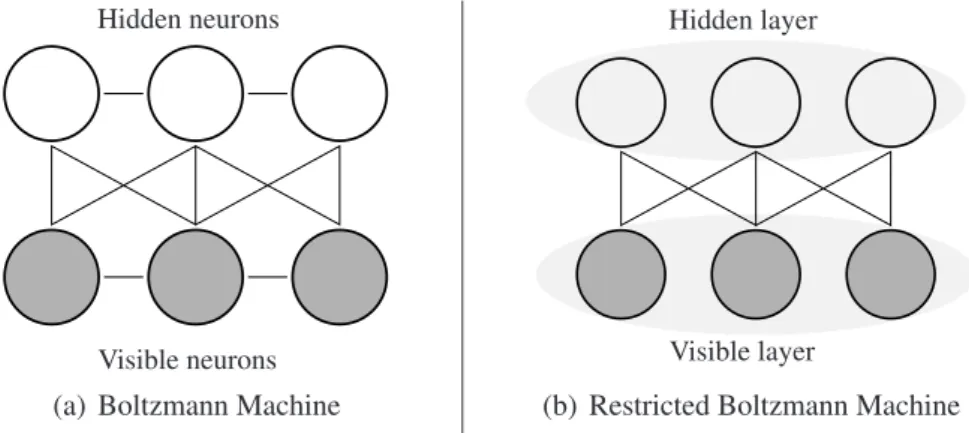
To overcome practical limitations imposed on the general Boltzmann machine such as the problem of inefficient sampling, a structurally restricted version of Boltzmann machine called Restricted Boltzmann Machine (RBM) has been proposed by Smolensky (1986). RBM is constructed by removing the lateral connections in-between the visible neurons and the hidden neurons. Therefore, a visible neuron would only have edges connected to the hidden neurons, and a hidden neuron would only have edges connected to the visible neurons. Now, the structure of RBM can be divided into two layers with inter-connecting edges. The relationship between BM and RBM is illustrated in Figure 2.1.

Although the imposed restriction could possibly suggest that the representational power might have been reduced, Le Roux & Bengio (2008) showed that RBM is a universal ap-proximator such that it can model any discrete-valued probability distribution (Le Roux & Bengio, 2008).

(23)

Hidden neurons

Visible neurons (a) Boltzmann Machine

Hidden layer

Visible layer

(b) Restricted Boltzmann Machine

Figure 2.1: Illustration of the relationship between Boltzmann machine and restricted Boltzmann machine

As the restriction has been imposed on the structure, the energy and the state probability must be modified accordingly:

E(v,h _|θ_{) =} ₋_vT_Wh₋_bT_v₋_cT_h _(2.7)

P(v,h_|θ_{) =} 1

Z(θ₎exp{−E(v,h|θ)},

where now parametersθ_{= (}_W,_b,_c₎_{include biases}_b_and_c_.

Since each hidden neuron is independent of each other given all the visible neurons, it is possible to explicitly sum out the hidden neurons and obtain the unnormalized probability of the visible neurons. The probability of a state of visible neuronsvis, then,

P(v_|θ_{) =} 1 Z(θ₎exp(b T v) nh Y j=1 1 + exp cj + nv X i=1 wijvi !! , (2.8)

wherenvandnh are the number of the visible neurons and the hidden neurons, respectively

(Salakhutdinov, 2009a).

2.2.1

Training Restricted Boltzmann Machine

The learning rules of RBM , then, become

wij ←wij +ηw hvihji_d− hvihji_m (2.9) bi ←bi+ηb[hvii_d− hvii_m] (2.10) cj ←cj +ηc hhji_d− hhji_m , (2.11)

(24)

where the same shorthand notation_h·i_P₍_·₎was used as before.

Although there is no rigorous theoretical background on choosing learning rates, tradition-ally, smaller learning rates are used for learning both biases (Hinton, 2010).

Since RBM is a special case of BM, it is possible to employ the same Gibbs sampling to learn. Thanks to its restricted structure, Gibbs sampling can be used more efficiently, as given one layer, either visible or hidden, the neurons in the other layer become mutually independent (see Figure 2.2). This possibility of the layer-wise sampling enables the full utilization of the modern parallelized computing environment.

Hidden layer

Visible layer

x0

h0∼p(h|x0) h1∼p(h|x1) h2∼p(h|x2)

x1∼p(x|h0) x2∼p(x|h1)

Figure 2.2: Visualization of the idea of how the layer-wise Gibbs sampling is done in RBM .

However, as the number of neurons in RBM increases, a greater number of samples must be gathered by Gibbs sampling in order to properly explain the probability distribution represented by RBM . Moreover, due to the nature of Gibbs samplings, the samples might still miss some modes of the distribution.

Many approaches have been proposed to overcome these difficulties.

2.2.2

Contrastive divergence learning

One popular approach is contrastive divergence (CD) learning proposed by Hinton (2002) as an approximate method for training Product-of-Expert models. Equation (2.8) directly implies that RBM is a special case of PoE models, and CD learning can readily be used for training RBMs.

CD learning approximates the true gradient by replacing the expectation over P(v,h _| θ₎

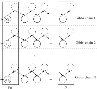
with an expectation over a distributionPnthat is obtained by runningnsteps of Gibbs

sam-pling from the empirical distribution defined by the training samples. Figure 2.3 illustrates the distributionsP0andPn.

For the weights, the CD learning formula, then, becomes

wij ←wij +η

hxihji_P₀ − hxihji_P_n

(25)

... ... ... ... ... ... ... x1 x2 xN p0 pn Gibbs chain 1 Gibbs chain 2 Gibbs chain N

Figure 2.3: Visualization of how CD learning obtains the empirical distribution used in the positive phase and the approximate model distribution used in the negative phase. In the figure, each row represents the Gibbs sampling chain starting from each training data sample, andp0 andpndenote the empirical distribution and the approximate model

distribution, respectively.

It should be noted that the casen = 0produces the empirical distributionP(h_{| {}v(t)_}_,_θ₎

used in the positive phase, whereas the case n = _∞produces the true distribution of the negative phaseP(x_|θ₎_{(Carreira-Perpiñán & Hinton, 2005; Bengio & Delalleau, 2009).}

As it can be anticipated from the fact that the direction of the gradient is not identical to the exact gradient, CD learning is known to be biased (Carreira-Perpiñán & Hinton, 2005; Bengio & Delalleau, 2009). Nevertheless, CD learning has been shown to work well in practice. A good property of CD is that in case the data distribution is multi-modal, running the chains starting from each data sample guarantees, that the samples approximating the negative phase have representatives from different modes.

This advantage of CD learning, however, is its disadvantage at the same time. The samples from Pn do not necessarily explain the whole state space. Hence, some of the modes in

the model distribution are not explored, and even after learning has converged the model distribution possesses the modes that are not in the data distribution defined by the training data set. This problem is illustrated in Figure 2.4.

In order to overcome this problem, different approaches based on CD learning have been proposed. Among them persistent contrastive divergence (PCD) learning is the simplest extension of CD learning (Tieleman, 2008).

(26)

model

data

(a) Model distribution and training samples (b) CD fantasy samples and training samples

Figure 2.4: The left figure shows the model distribution (blue) and and the training samples (black dots). The blue dots in the right figure indicates the fantasy particles obtained by CD learning. It is apparent that the fantasy particles failed to explain the whole space by missing the mode at the top.

At every gradient update step, CD learning performs the Gibbs sampling starting from the training data samples, whereas PCD learning begins the sampling from the model samples obtained at the last gradient update. In this way, it is expected for the model samples to explore the modes in the model distribution that are not close to the training samples. However, PCD learning still suffers from missing the modes in the model distribution as learning progresses. It is due to the poor mixing of the Gibbs sampling which produces the highly-correlated samples for successive gradient updates. This behavior makes the approaches based on CD learning to suffer from the divergence of the likelihood (Schulz et al., 2010; Fischer & Igel, 2010; Desjardins et al., 2010b,a) if learning is performed with-out carefully and manually chosen learning heuristics such as learning rate schedule, weight decay, and momentum.

Numerous approaches based on CD learning, other than PCD learning, have been proposed recently. For instance, Fast PCD learning proposed by Tieleman & Hinton (2009) extends PCD learning by maintaining fast weights that help obtaining better model samples.

2.2.3

Learning based on advanced MCMC sampling methods

Instead of approximating the gradient direction, it is possible to apply more sophisticated MCMC sampling methods other than simple Gibbs sampling.

One alternative to the Gibbs sampling is parallel tempering (PT) sampling (Earl & Deem, 2005) which was recently proposed as a replacement for Gibbs sampling in training RBMs

(27)

by Desjardins et al. (2010b) and Cho et al. (2010). The detailed description of PT and how PT is used for training RBMs is given in Chapter 3 with the experiments showing the superiority of PT learning compared to CD learning.

In addition to PT learning, other approaches based on advanced MCMC sampling methods have also been proposed. For instance, stochastic approximation procedure based on tem-pered transition (Neal, 1994) is one that was proposed recently by Salakhutdinov (2009b) that utilizes multiple chains of Gibbs sampling with different temperatures. A hybrid Monte Carlo algorithm (HMC) also has been successful in training more sophisticated RBMs such as a factored 3-way RBM (Ranzato et al., 2010) and an energy-based model (Teh, 2003), recently.

2.2.4

Other approaches

The approaches presented so far are based on the stochastic approximation using MCMC sampling. However, there exist other approaches for training RBMs.

One approach is to approximate the likelihood function with the pseudo-likelihood (Be-sag, 1975), and thus, training RBMs becomes maximizing the pseudo-likelihood. The log-pseudo-likelihood function given a data set_{v(t)_}N

t=1is defined as fPL(θ_{) =} 1 N N X t=1 d X i=1 logP(v(_it)_|v(_\t_i)),

wherex\idenotes a vector[x1,· · · , xi−1, xi+1,· · · , xd]T as before. The hidden neurons can

be explicitly summed out by Equation (2.8)

The maximum pseudo-likelihood (MPL) learning approximate the joint probability distri-bution of RBM with the product of one-dimensional probability distridistri-butions. Although it removes the necessity of computing the intractable normalizing constant, MPL learning tends not to work well neither with RBMs nor BMs (Marlin et al., 2010; Salakhutdinov, 2009b), as it does not approximate the maximum likelihood estimator (MLE) well except for some extreme cases (Geyer, 1991).

Another approach, ratio matching (RM) was recently proposed by Hyvärinen (2007). In-stead of the likelihood, RM considers ratios of probabilities. The data ratio which is defined by the ratio between the probability of a given observation and the probability of the obser-vation vector with one variable i flipped as in Equation (2.12), and the model ratio is the same ratio under the model distribution. RM learning tries to force the data and model ratio

(28)

as close as possible.

RM is beneficial as the ratio does not require the computation of the normalizing constant, as P(v) P(v¬i) = P ∗₍_v₎ P∗₍_v ¬i) , (2.12)

wherev¬iis equivalent tovwith thei-th component flipped.

Additionally, recently proposed generalized score matching (Lyu, 2009) can be used to train RBMs.

These approaches have been compared to each other and to the stochastic approximation by Marlin et al. (2010). However, these learning methods suffer from the computational complexity when the dimensionality of the observations is large, and they do not show sig-nificant improvement over the stochastic approximation based on MCMC sampling. Hence, this thesis only considers stochastic gradient-based method using MCMC sampling.

2.3

Evaluating Restricted Boltzmann Machines

2.3.1

Likelihood and Annealed Importance Sampling

A natural way to assess the performance of a trained RBM is to compute the likelihood of the model and the probabilities of test data samples under the trained RBM. Also, as will be discussed in Chapter 3 and was shown in the author’s paper (Cho et al., 2010), the probability of the random data samples also can be used as a measure of the goodness of RBMs.

Due to the structural restriction, explicitly summing out the hidden neurons is fairly straight-forward (see Equation (2.8),) however, unfortunately computing the probability of an ob-servation is still intractable due to the normalizing constant. The normalizing constant can only be computed exactly by summing exponentially many terms, and unless the dimen-sionality of the data set is very small, it is simply impossible. Thus, instead of exactly computing it, an approximate method must be employed.

For estimating the normalizing constant, this thesis uses annealed importance sampling (AIS) (Neal, 1998) which has been successfully employed for computing the normalizing constant of RBM (Salakhutdinov, 2009b).

(29)

of two normalizing constants. For two probability densitiesPA(x) = P∗ A(x) ZA andPB(x) = P∗ B(x)

ZB , the ratio of two normalizing constantsZAandZBcan be estimated by a Monte Carlo

sampling method without any bias if it is possible to sample fromPA(·):

ZB ZA =EPA P∗ B(x) P∗ A(x) ≈ 1 M M X i=1 P∗ B(xi) P∗ A(xi) , (2.13)

wherexiare samples fromPA(x). The quality of the approximation in terms of the variance

depends highly on how closePA(·)andPB(·)are. IfPA(·)is not near-perfect

approxima-tion toPB, then the variance of the estimate can be as large as infinity.

Based on SIS, AIS estimates the normalizing constant of the model distribution by comput-ing the ratio of the normalizcomput-ing constants of consecutive intermediate distributions rangcomput-ing from so-called base distribution and the target distribution. The base distribution is chosen such that its normalizing constant Z0 can be computed exactly and it is possible to collect

independent samples from it. A natural choice of the base distribution for RBM is RBM with zero weightsW. This yields the normalizing constant

Z0 = Y i (1 + exp{bi}) Y j (1 + exp{cj}),

where indicesiandj go through all the visible and hidden neurons, respectively.

By computing the product of the estimated ratios of the intermediate normalizing constants and Z0, the normalizing constant of the target RBM can be estimated. The algorithm

im-plementing AIS is outlined in Algorithm 2.

The presented algorithm describes constructing intermediate RBMs following what Salakhut-dinov (2009a) proposed. The base distribution is represented by RBM with zero weights, but biases that are identical to those of the target RBM. However, it should be noticed that there are other possibilities for constructing intermediate distributions and choosing a base distribution. For instance, in the following chapters, the base distribution is an RBM with both zero weights and zero biases such that there is no need for each intermediate RBM to maintain twice as many hidden neurons as the target RBM has.

2.3.2

Classification accuracy and other measures

It is evident from the previously mentioned research papers utilizing deep neural networks built from the stack of RBMs (Salakhutdinov, 2009b; Hinton & Salakhutdinov, 2006) that the hidden activation probabilities of RBM trained on the data set could improve the

(30)

classi-Algorithm 2Estimating the normalizing constant by annealed importance sampling Create a sequence of temperaturesTksuch that0 =T0 < T1 <· · ·< TK = 1.

Create a base RBMR0 with parametersθ0 = (W0,b,c), whereW0 = 0.

Create a sequence of intermediate RBMsRk such that

• It has twice as many hidden nodes as the target RBM has.

• Parameters areθ_k _{= ([(1}₋_T_k₎_W₀ _T_k_W_]_,_[(1₋_T_k₎_b₀ _T_k_b_]_,₍₁₋_T_k₎_cT 0 TkcT T ). form = 1· · ·M do Samplex₁fromR0. fork= 1_{· · ·}K₋1do

Samplexk+1 fromRk by one-step Gibbs sampling starting fromxk.

end for Setum = QK k=1 P∗ k(xk) P∗ k−1(xk), whereP ∗

k(·)is an unnormalized marginal distribution

func-tion ofRk. end for The estimate of ZK Z0 is 1 M PM m=1um.

fication accuracy compared to classifying the data set based on its raw features. However, these approaches often require the discriminative fine-tuning which destroys the generative structure of RBM .

Fortunately, recent papers suggest that the hidden activation probabilities of RBM which was trained in a unsupervised manner also help the classification task. Krizhevsky (2009) successfully used a Gaussian-Bernoulli RBM to extract features from images that help ob-taining high classification accuracy. Also, more sophisticated forms of RBM introduced recently (Ranzato & Hinton, 2010; Ranzato et al., 2010; Osindero & Hinton, 2008) were shown to be able to extract features that are more useful for the classification task.

Furthermore, Coates et al. (2010) showed that features extracted by the probabilistic mod-els learned in an unsupervised way outperforms the supervised counter-parts such as con-volutional neural networks (LeCun et al., 1998) and concon-volutional deep belief network (Krizhevsky, 2010).

Thus, it is sensible to use the classification accuracy of the trained RBM as a performance measure.

Additionally, thanks to its bipartite structure and the layer-wise Gibbs sampling, the recon-struction error could also be used as a measure for the performance assessment (Hinton, 2010). A reconstruction error is defined as

E(x) =_kx₋x1k2,

(31)

(a) Test samples

(b) Before training (_E= 203.7805₎

(c) After 1 epoch (_E= 26.5676₎

(d) After 5 epochs (_E= 20.9808₎

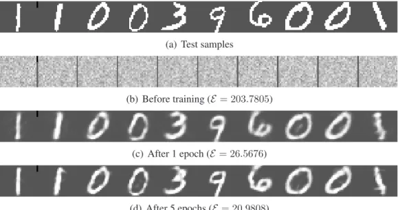
Figure 2.5: Examples of reconstruction errors for RBM with 100 hidden neurons applied to MNIST handwritten digits. The figure shows randomly selected sample digits (a) and their reconstructions (b-d). The reconstruction errors _E on the whole test data set are shown inside the brackets. Reconstructions are shown using the activation probabilities rather than the actual activations which are the samples collected based on the activation probabilities.

example of how reconstruction error decreases during training is given in Figure 2.5. However, these measures are not directly reflecting the true quality of RBM , since training neither maximizes nor minimizes any of these measures. Therefore, for the rest of this thesis, the experiments mostly assess the trained RBM by the likelihood of the model and the probabilities of the test samples given the model.

2.3.3

Directly visualizing and inspecting parameters

Lastly, one way to analyze the quality of a trained model is to look at the features (the weightswij) and the bias termscj corresponding to different hidden neurons of the trained

RBM. It especially helps when training data samples consist of images that can be readily visualized.

For instance, features of RBM trained on handwritten digits can be visualized as shown in Figure 2.6. Each feature, or filter, resembles a part of digits, or a combination of parts of digits. When learning fails, it is easy to observe degenerate features that are noisy global features.

(32)

to the modeling capacity of RBM . Neurons that have a large bias cj are most of the time

active, and they are not very useful, as the weights associated to them can be incorporated into the bias termb. On the other hand, hidden neurons that are mostly inactive (e.g., with large negative biases cj) or whose activations are independent of data are also useless, as

the learning capacity of the RBM does not change even if they are removed.

Like other indirect measures presented previously, the visualization and inspection of pa-rameter values must be performed carefully. There is no objective measure for the quality of the visualized features, and the visualized features and the values of biases may evolve slowly over training.

2.4

Difficulties and conventional remedies

2.4.1

High variance in resulting RBMs and divergence

The fact that the target function cannot be computed exactly during learning makes training RBMs difficult. It is computational infeasible to tell when the learning has converged, or even it is not easy to tell whether the learning is actually happening. Furthermore, it is not possible to use any advanced gradient method such as non-linear conjugate gradient. Since learning is performed using stochastic gradient updates, it converges to a local solu-tion. The problem is that it is not feasible to compare the different solutions analytically, and choose the best one among them. Schulz et al. (2010) and Fischer & Igel (2010) re-cently showed that depending on the initialization and the learning parameters the resulting RBMs vary highly even on the small toy data sets.

More problematically, most approximate approaches presented in the previous sections have been shown to diverge, if the learning parameters were not chosen appropriately (Des-jardins et al., 2010b; Schulz et al., 2010; Fischer & Igel, 2010). The use of a better MCMC sampling method, e.g. parallel tempering, has been shown to better avoid the diverging behavior, but in a long run without using the appropriate learning rate scheduling, the log-likelihood fluctuates highly (Desjardins et al., 2010b, 2009) which is not desirable.

2.4.2

Existence of possibly meaningless hidden neurons

It has been shown that RBM is a universal approximator so that with enough number of hid-den neurons it can model any discrete-valued probability distribution (Le Roux & Bengio,

(33)

2008).

However, in practice, the number of hidden neurons is always limited, and depending on learning procedures, not all hidden neurons contribute to the representational power of RBM .

For instance, those hidden neurons that are always active are meaningless, since the weights associated to them can be incorporated into bias terms. Also, any hidden neuron that is inac-tive always is meaningless, since then, the removal of the hidden neuron does not affect the modeling capacity of RBM at all (see Section 2.3.3 for details on determining meaningless hidden neurons.)

Ideally, each hidden neuron should represent a distinct “meaningful” feature, for example, a typical part of the image. We have noticed, however, that very often the hidden neurons tend to learn features that resemble the visible bias termb. This effect is more prominent at the initial stage of learning and for data set in which visible bits are mostly active, such as 1-MNIST where each bit of MNIST handwritten data set was flipped.

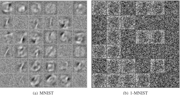
Figure 2.6(b) presents an example how RBM can be ill-trained when the learning param-eters were not carefully chosen and the training samples were dense in a sense that the number of ones in each training sample is much more than that of zeros. The RBM with 36 hidden neurons were learned on 1-MNIST which is a very dense data set compared to the original MNIST.

18 hidden neurons were not able to learn any useful features, and they are mostly inactive. The other 18 neurons are mostly active, and as anticipated, learned global features that somewhat resemble the visible bias.

Even when the training data samples are not dense, with the small number of hidden neu-rons, inappropriate choice of learning parameters, and inappropriate choice of initialization of the parameters, many hidden neurons will be useless. The visualization of the filters learned by RBM with 36 hidden neurons trained on MNIST with the constant learning rate0.1and the initial weights sampled from the uniform distribution between₋1and1is shown in Figure 2.6(a). In the figure, about 20 neurons out of 36 neurons look as if they learned some useful features. However, there still exist those neurons that are either mostly active or mostly inactive.

2.4.3

Conventional remedies

(34)

(a) MNIST (b) 1-MNIST

Figure 2.6: Visualization of filters learned by RBMs with 36 hidden neurons on MNIST and 1-MNIST after 5 epochs using traditional learning algorithms.

1)Learning rate scheduling: Due to its stochastic nature (when only part of data, i.e. mini-batch, is used to compute the gradient), the gradient does not tend to approach zero. There-fore, the learning rate is typically forced towards zero at the end of training. However, if the learning rate is annealed too quickly, then the RBM will not learn anything, but only stay in the plateau of the learning space where most of the weights stay close to zero.

2)Weight decayprior regularizes the indefinite growth of the norm of the parameters, which sometimes happens in practice. This yields the following update rules:

wij ←wij +η

hxihji_P₀ − hxihji_P_n−αwij

,

3)Momentumis used to smoothen the gradients yielding a modified update rule:

wij ←wij +η

(1−β)∇wij,t+β∇wij,t−1

,

where_∇wij,tand∇wij,t−1 are the gradients computed at the current and previous iterations

and0≤β <1is a momentum parameter.

4) In order to avoid having meaningless hidden neurons, there have been attempts to spar-sify the activations of the hidden neurons (Hinton, 2010; Lee et al., 2008). The sparsity can be achieved by adding a regularization term that penalizes a deviation of the expected

(35)

activation from a fixed levelp:

ρX

j

|p− hhji_P₀|2,

whereρdenotes a degree of regularization.

The proposed heuristics are known to help in many practical applications. However, they all introduce extra parameters which should be selected very carefully. Good values of these parameters are typically found by trial and error and it seems that one requires a lot of experience to set the learning settings right (Hinton, 2010). The stochastic gradient learning of RBM can easily diverge even when the proposed heuristics are used, if the associated parameters are not chosen carefully (Schulz et al., 2010; Fischer & Igel, 2010).

(36)

Chapter 3

Parallel Tempering Learning

While contrastive divergence learning has been considered an efficient way to learn RBM , it has a drawback due to a biased approximation in the learning gradient. This chapter proposes to use an advanced Monte Carlo method called parallel tempering instead, and shows experimentally that it works efficiently. A part of the work described in this chapter was reported in the author’s paper (Cho et al., 2010).

3.1

Parallel Tempering and Restricted Boltzmann Machines

Training RBMs using the stochastic gradient updates requires that it must be possible to efficiently sample from the data distribution P(h _| v,θ₎ _{and the model distribution}

P(v,h _| θ_{). Thanks to the simple structure and formulation of BM and RBM , a Gibbs}

sampling is enough to obtain the samples. However, its inefficiency led to the contrastive divergence (CD) learning and its variants which do not follow the exact gradient, but rather, approximate the exact gradient. Its nature of simplicity and computational efficiency made the CD learning huge success in training RBMs, but still the CD learning has disadvantages. For more detailed discussion on the topic, Chapter 2 should be referred.

A problem that has not been addressed neither by Gibbs sampling nor by CD learning is that the samples generated during the negative phase do not tend to explain the whole state space. This section, therefore, proposes to use another improved variant of Markov-Chain Monte Carlo sampling method calledparallel tempering(PT).

(37)

3.1.1

Parallel Tempering

The introduction of PT sampling goes back to 1980s when Swendsen & Wang (1986) intro-duced a replica Monte Carlo simulation and applied it to the Ising model which is equiva-lent to a Boltzmann machine with only visible neurons. The replica Monte Carlo simulation proposed to simulate multiple copies of particles (replica) with different temperature con-currently rather than simulating them sequentially. Similarly, Geyer (1991) later presented applying parallel chaining of MCMC sampling based on the speed of mixing of samples across parallel chains to the maximum likelihood estimator.

Afterward, there have been many approaches of applying parallel tempering to other fields. Those fields include the simulations of polymers, proteins, and states of solid materials, and even, studies of phase transitions at the quantum levels (for more applications, see Earl & Deem, 2005).

In the rest of this section, PT sampling having multiple Gibbs sampling chains with varying levels of temperatures used to obtaingoodsamples from the state space is briefly discussed. The basic idea of PT sampling is that samples are collected from multiple chains of Gibbs sampling with different temperatures1. The term temperaturein this context denotes the level of the energy of the overall system. The higher the temperature of the chain, the more likely the samples collected by Gibbs sampling move freely.

For every pair of collected samples from two distinct chains, the swap probability is com-puted, and the samples are swapped according to the probability. The swap probability of a pair of samples is formulated according to the Metropolis rule (see, e.g., Mackay, 2002) as

Pswap(xT1,xT2) = min 1,PT1(xT2)PT2(xT1) PT1(xT1)PT2(xT2) , (3.1)

whereT1andT2denote the temperatures of the two chains, andxT1 andxT2denote samples

collected from the two chains.

After each round of sampling and swapping, the sample at the true temperature T = 1 is gathered as the sample for the iteration. The samples come from the true distribution ,

P(v,h_|θ₎_{in case of RBMs, assuming that enough iterations are run to diminish the effect}

of the initialization.

It must be noted that the Gibbs sampling chain with the highest temperature (T = 0) is never

1_{Since the lower value denotes the higher temperature, a term} _{inverse temperatures} _{from the highest}

temperature T = 0_{to the current temperature} T = 1 _{is frequently used, but in this thesis,} _temperature

(38)

multi-modal such that all the neurons are mutually independent and likely to be active with probability 1₂. So, the samples from the chain are less prone to missing some modes. From the chain with the highest temperature to the lowest temperature, samples from each chain become more and more likely to follow the target model distribution. How PT sampling could avoid being trapped into a single mode is illustrated in Figure 3.1.

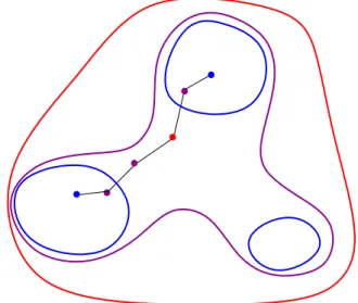
Figure 3.1: Illustration of how PT sampling could avoid being trapped in a single mode. The red, purple, and blue curves and dots indicate distributions and the samples from the distributions with the high, medium, and cold temperatures, respectively. Each black line indicates a single sampling step.

This nature of swapping samples between the different temperatures enables better mixing of samples from different modes with much less number of samples than that would have been required if Gibbs sampling was used.

3.1.2

Parallel Tempering Learning

PT sampling in training RBMs can be simply uses as a replacement of Gibbs sampling in the negative phase. This method is, from now on, referred to as PT learning. Due to the previously mentioned characteristics, it is expected that the samples collected during the negative phase would explain the model distribution better, and that the learning process would be successful even with a smaller number of samples than those required if Gibbs sampling is used.

A brief description of how PT sampling can be carried out for RBMs is given in Algorithm 3. This is the procedure that is run between each parameter update during learning.

(39)

Algorithm 3PT sampling steps for an RBM

Create a sequence of RBMs (R0, R1,· · · , RK) such that parameters of Rk are θk =

(TkW, Tkb, Tkc), where0≤T0 < T1 <· · ·< TK = 1.

Create an empty set of samplesX ₌_{}_.

Setx0 = (x0,0,· · · ,xK,0)such that everyxk,0 is a uniformly distributed random vector

(or use old ones from the previous epoch).

form = 1· · ·M do

Samplexm = (x0,m,· · · ,xK,m)from the sequence of RBMs such thatxk,mis sampled

by one-step Gibbs sampling starting fromxk,m−1.

forj = 2· · ·K do

Swapxj,mandxj−1,maccording toPswap(xj,m,xj−1,m)computed using (3.1).

end for

AddxK,mtoX.

end for

X _{is the set of samples collected by parallel tempering sampling.}

3.2

Experiments

Two different sets of experiments were made. The goal of the first set of experiments was to test the capability of RBMs to capture the data distribution. Samples were generated from the RBM trained on the OptDigits data set. The data set was acquired from the UCI Machine Learning Repository (Asuncion & Newman, 2007) and it consisted of handwritten digits of the size8×8pixels. The samples were collected by parallel tempering sampling starting from a randomly drawn state. Most of the samples were observed to resemble the digits regardless of the initial state.

The second set of experiments was conducted in order to compare the performance of RBMs depending on two different learning methods: CD learning and learning using sam-pling with PT. The performance was evaluated by the estimated likelihood of the training data set and the estimated probability of the test data set, both computed by annealed im-portance sampling (AIS).

Furthermore, in the second experiment the probability of uniformly randomly generated data is computed for the current RBM model. The goal was to observe a potential problem of CD learning that the samples generated during the negative phase do not represent the state space as well as the samples generated by PT sampling, but only represent the region centered around the training samples (Bengio, 2009). The probability of random data was computed for different learning methods and compared.2

2

We assume that uniformly drawn samples do not lie close to the training data because the size of the training data set is much smaller than the size of the state space which is264_.

(40)

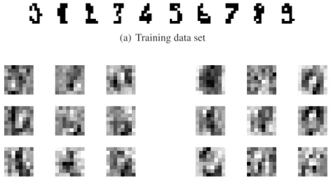
(a) Training data set

(b) Visualization of hidden nodes (CD1) (c) Visualization of hidden nodes (PT)

Figure 3.2: Training data set and visualization of hidden nodes. (a): 10 training samples where for each digit one sample was randomly chosen. (b) (c): the weights associated with nine randomly chosen hidden neurons.

3.2.1

Generating samples from a trained restricted Boltzmann

ma-chine

RBMs were constructed such that there are 64 visible neurons and 100 hidden neurons. Each RBM was trained with 3822 training samples of8_×8handwritten digits. The original OptDigits data set provides 17-level greyscale digits, but for simplicity the intensity of each pixel was rounded so that the intensity less than 8 became 0 (and 1 otherwise).

Each RBM was trained separately by CD learning with n = 1and learning with PT sam-pling. PT sampling was done withK = 20temperaturesT0 = 0, T1 = 0.05, . . . , T20 = 1.

The models represented by the RBMs are named CD1 and PT, respectively. Each gradient update was done in the full-batch style so that all the training samples were used. CD1 and PT were trained for 2000 epochs, and the learning rate η started from 0.05 and gradually decreased following the search-then-converge scheduling such that the learning rateη(t)at thet-th update is

η(t) = η(0) 1 + t

t0

,

whereη(0) = 0.05for both the weight and the bias, andt0 = 300for both CD1 and PT.

Figure 3.2 shows the training data samples and the visualization of the hidden nodes after training. The visualization of the hidden node was done by displaying the weights

(41)

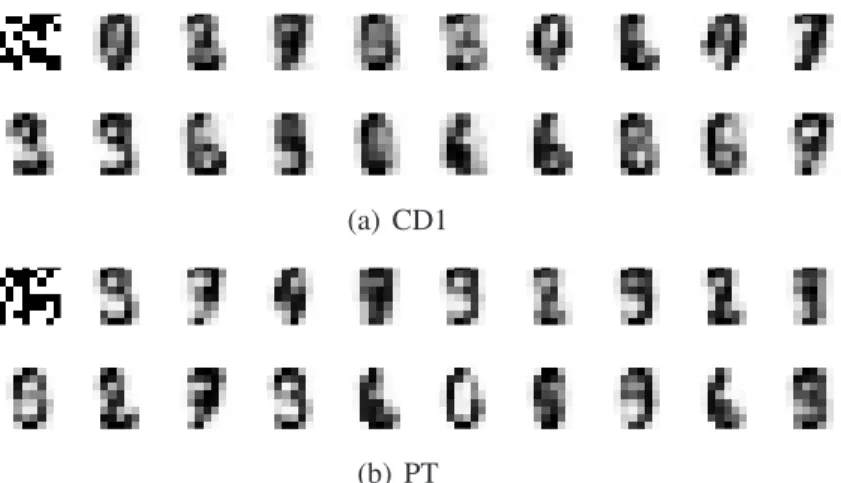
associ-(a) CD1

(b) PT

Figure 3.3: Samples generated by parallel tempering sampling from the RBM trained with (a) CD1 and (b) PT started from the random sample. The first digits of both figures are the random initial samples.

ated with the node as a grey-scale digit. It can be observed that each hidden node represents a distinct feature.

Figure 3.3 shows the activation probabilities for the visible neurons of the generated sam-ples from the models learned with CD1 and PT. The digits in the figure are 19 samsam-ples chosen out of 2000 samples collected by PT sampling starting from the random sample. Each consecutive samples are separated by 100 sampling steps, and the first digit in both figures of Figure 3.3 represents the random initial sample. It is clear that the trained RBM is able to generate digits which look similar to the training data regardless of the training methods.

3.2.2

Comparison between CD learning and PT learning

For the second experiment, RBMs with 100 hidden neurons were trained using four learning algorithms: CD1, CD5, CD25 and PT, where CDn denotes CD learning with n Gibbs sampling steps per gradient update.

The parameters K and M of parallel tempering were chosen so that the number of total Gibbs sampling steps during one gradient update matches that of CD1 which uses as many samples as the number of the training data samples. PT was, therefore, trained withK = 20 temperatures andM = 192samples per gradient update. This choice is reasonable in the sense that the difference in CD learning and learning with PT sampling only depends on the number of Gibbs sampling steps, whereas the computational cost of additional operations may vary largely depending on the implementation.

(42)

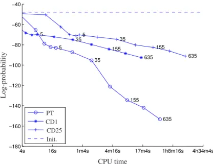
4s 16s 1m4s 4m16s 17m4s 1h8m16s 4h34m4s −50 −45 −40 −35 −30 −25 −20 −15 −10 5 35 155 635 5 35 155 635 5 35 155 635 L o g -p ro b ab il it y CPU time PT CD1 CD25 Init.

Figure 3.4: Average probabilities of test data against the processor time. The dashed line indicates the initial log-likelihood. The numbers denote the number of epochs after which the value was measured.

Each RBM was trained for 635 epochs and the probabilities of both training and test data were estimated. 50AIS runs with5000temperatures were averaged to obtain the estimate of the normalizing constants. All the models were trained 30 times and the averaged per-formance indices were calculated.

Figure 3.4 and Figure 3.5 show that the probability of the test data and the likelihood of the model increase, while the probability of the random data decreases over the gradient updates. This is consistent with the fact that the gradient maximizes the likelihood accord-ing to the distribution of the trainaccord-ing data. Figure 3.6 confirms that the probability of the unseen samples that are not close to any training sample is decreased.

However, the rate of the changes in the likelihood and the probability of the test data over updates differs from one model to another. PT achieves the highest average likelihood and the highest average probability of the test data, and at the same time achieves the lowest probability of the random data at the fastest rate. It can be further observed that PT learning is computationally more favorable than CD25 and comparable to CD1.

Figure 3.7 shows the average probability of the test data set and the random data set by 30 independent trials. These results confirm that PT indeed achieves the highest probability of the test data set and the lowest probability of the random data set. It should be, however, noted that the variance of PT is greater than those of both CD1 and CD25.

(43)

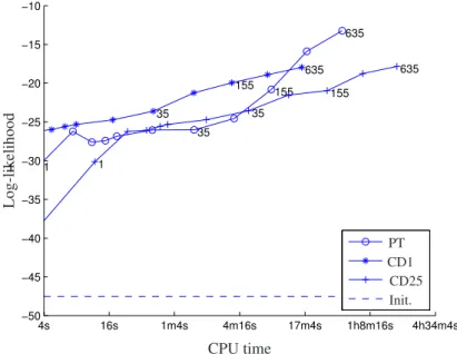
4s 16s 1m4s 4m16s 17m4s 1h8m16s 4h34m4s −50 −45 −40 −35 −30 −25 −20 −15 −10 1 35 155 635 1 35 155 635 1 35 155 635 L o g -l ik el ih o o d CPU time PT CD1 CD25 Init.

Figure 3.5: Average log-likelihood of the model against the processor time. The dashed line indicates the initial log-probability of test data. The numbers denote the number of epochs after which the value was measured.

The increase ofnin CD learning certainly boosts up the rate of the increase in the likelihood as a function of learning epochs, but even withn = 25CD learning cannot achieve as large likelihood as PT does. CD learning withn= 25is much more computationally demanding than PT. This result indicates that the use of the advanced sampling technique can yield faster and better training of RBMs.

3.3

Practical Consideration

Although the experiments showed that gathering enough number of samples from a single PT sampling chain consisting of multiple parallel Gibbs sampling chain is sufficient to train RBMs, PT learning showed its weakness evidenced by the large variance of the resulting RBMs with different initializations.

In order to reduce the high variabilities in training RBMs, PT learning can borrow the idea from CD and PCD learning introduced in Chapter 2 such that there are multiple sets of multiple Gibbs sampling chains starting from the training samples in the initial minibatch, or full-batch. For each update,nsteps of PT sampling is performed starting from the model samples obtained in the previous update. For every nswap updates, the swapping of the

(44)

4s 16s 1m4s 4m16s 17m4s 1h8m16s 4h34m4s −180 −160 −140 −120 −100 −80 −60 −40 5 35 155 635 5 35 155 635 5 35 155 635 L o g -p ro b ab il it y CPU time PT CD1 CD25 Init.

Figure 3.6: Average probabilities of random data against the processor time. The dashed line indicates the initial log-probability of random data. The numbers denote the number of epochs after which the value was measured.

samples can be performed, wherenswapis a small positive integer3.

Although the experimental results with this modification are not presented in this chapter, it is clear from the experiments in Chapter 4 and Chapter 5 that the variance is reduced significantly when the modification is employed.

3.4

Conclusions

This chapter proposed an alternative approach which utilizes parallel tempering for training RBMs. This approach does not sacrifice the optimality of the direction of the gradient, as CD learning does, but reduces the computational cost by improving the quality of the samples.

Two separate experiments were done for (1) confirming the capability of RBM to capture the data distribution and (2) showing that RBM trained by the proposed PT approach is superior to that trained by the conventional CD learning. The former experiment confirmed that RBM trained by either CD learning or learning with PT sampling is able to generate samples resembling the training data. The second