DigitalCommons@WayneState
Wayne State University Dissertations1-1-2010
Localized Feature Selection For Unsupervised
Learning
Yuanhong Li
Wayne State University,
Follow this and additional works at:http://digitalcommons.wayne.edu/oa_dissertations
This Open Access Dissertation is brought to you for free and open access by DigitalCommons@WayneState. It has been accepted for inclusion in Wayne State University Dissertations by an authorized administrator of DigitalCommons@WayneState.
Recommended Citation
by
YUANHONG LI DISSERTATION
Submitted to the Graduate School of Wayne State University,
Detroit, Michigan
in partial fulfillment of the requirements for the degree of
DOCTOR OF PHILOSOPHY
2010
MAJOR: COMPUTER SCIENCE Approved by:
First and foremost, I want to express my greatest appreciation to my supervisor, Dr. Ming Dong. Under his guidance, I have learned a lot in different aspects of conducting research, including finding a good research topic and writing convincing technical paper. It is his guid-ance, support and tremendous help that made this dissertation possible. I am also very thankful to the rest of my thesis committee, including Dr. Jing hua, Dr. Hao Ying, and Dr. Chandan Reddy. Their advice and suggestions have been very helpful.
I want to thank Dr. Manjeet Rege, Dr. Changbo Yang, Dr. Xuanwen Luo, Yanhua Chen and Lijun Wang for their enthusiastic help during my Ph.D. study, which I shall never forget.
Let me express my special thanks to my wife, Dr. Hua Gu. Whithout her support and love, I could not complete my doctoral degree.
Acknowledgments . . . ii
List of Tables . . . vi
List of Figures . . . viii
Chapter 1 Introduction . . . 1
1.1 Data Representation . . . 1
1.2 Categories of Machine Learning Methods . . . 1
1.3 Dimensionality Reduction . . . 2
1.3.1 Feature Extraction . . . 3
1.3.2 Feature Selection . . . 3
1.4 General Procedure of Feature Selection . . . 3
1.4.1 Subset Generation . . . 4
1.4.2 Subset Evaluation . . . 5
1.4.3 Stopping Criteria . . . 5
1.4.4 Result Validation . . . 6
1.5 Categories of Feature Selection Algorithms . . . 6
1.5.1 Filter Approach . . . 7
1.5.2 Wrapper Approach . . . 7
1.5.3 Hybrid Approach . . . 7
1.6 Localized Feature Selection for Clustering . . . 7
1.6.1 Co-clustering . . . 9
1.6.2 Subspace Clustering . . . 9
1.7 Overview . . . 9
Chapter 2 Related Work in Unsupervised Feature Selection . . . 11
2.1 Global Feature Selection . . . 11
2.1.1 Filters . . . 11 iii
2.2 Localized Feature Selection . . . 16
2.2.1 Co-clustering . . . 16
2.2.2 Subspace Clustering . . . 19
2.3 Summary . . . 23
Chapter 3 Normalized Projection . . . 24
3.1 Introduction . . . 24
3.2 Evaluation Criteria . . . 26
3.2.1 Penalty of Overlapping and Unassigned Points . . . 29
3.2.2 Unassigned/New data . . . 31
3.3 Search Methods . . . 32
3.4 Experiment and Results . . . 33
3.4.1 Synthetic data . . . 35
3.4.2 Iris data . . . 36
3.4.3 Other UCI data . . . 38
3.4.4 UCI data with estimation ofk and initial clusters . . . 39
3.5 Summary . . . 41
Chapter 4 Localized Feature Selection with Maximal Likelihood Method . . . 42
4.1 Background on EM-based Clustering and Global Feature Selection . . . 42
4.2 Detecting Clusters Embedded in Feature Subspace . . . 44
4.2.1 Localized Feature Saliency . . . 44
4.2.2 Model Selection Based on Minimum Message Length (MML) . . . 47
4.2.3 Computational Complexity . . . 49
4.3 Experimental Results . . . 49
4.3.1 Synthetic Data . . . 50
4.3.2 Real-world datasets . . . 52
4.4 Summary . . . 55
Chapter 5 Simultaneous Localized Feature Selection and Model Detection for Gaus-sian Mixtures via Variational Learning . . . 58
5.1 Variational Approximation . . . 58
5.2 Local feature saliency with variational learning . . . 60
5.3 Computational Complexity . . . 66
5.4 Advantages of the proposed approach . . . 67
5.5 Experimental Results . . . 67
5.5.1 Synthetic Data . . . 68
5.5.2 Real-world datasets . . . 72
5.6 Summary . . . 76
Chapter 6 Conclusions and Recommendations for Future Work . . . 77
6.1 Conclusions . . . 77 6.2 Future work . . . 78 References . . . 79 Abstract . . . 88 Autobiographical Statement . . . 90 v
Table 3.1: Confusion matrix and error rate on the synthetic data. C1 - C4 are the output cluster labels, and T1 - T4 are the true cluster labels . . . 35
Table 3.2: Feature subset distribution on the synthetic data. C1 - C4 are the output
cluster labels. . . 35
Table 3.3: Confusion matrix and error rate on iris data. C1 - C3 are the output cluster
labels, and T1 - T3 are the true cluster labels . . . 36
Table 3.4: Feature subset distribution on iris data. C1-C3 are the output cluster labels. 36
Table 3.5: Comparison of k-means, GFS-k-means and LFS-k-means on other UCI
data sets . . . 38
Table 3.6: UCI datasets with estimated number of clusters and initial centroids. GFS:
Global feature selection and clustering by algorithm of [1]. ˆk: Estimated
number of clusters by GFS. LFS: Local feature selection by the proposed
algorithm withˆkand initial centroids obtained by GFS. . . 39
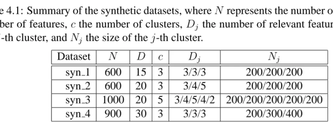
Table 4.1: Summary of the synthetic datasets, whereN represents the number of
pat-ters, Dthe number of features,cthe number of clusters,Dj the number of
relevant feature respecting to the j-th cluster, and Nj the size of the j-th
cluster. . . 50
Table 4.2: Results on the synthetic datasets. Saliency in the range [0, 1] is mapped
to gray-scale [0, 255] linearly. For the clustering with localized feature saliency, each image is a mapping of feature saliency of one cluster, where rows and columns of pixels represent runs and features, respectively. The separated row pixels above an image represent the true relevant features. The global feature saliency is illustrated in the same way. . . 51
Table 4.3: Summary of UCI datasets . . . 52
Table 4.4: Cluster numbers and pseudo error rates for UCI datasets. . . 53
Table 4.5: Feature saliency. Each image is a mapping of feature saliency for a
clus-ter, with exception that the highlighted one represents the global feature saliency. Saliency values [0,1] are linearly mapped to gray-scale [0,255]. Each row represents a run, and each column represents a feature. . . 56
Table 4.6: Attributes for the Boston housing data. . . 57
Table 5.1: Statistical summary on 100 synthetic datasets. . . 70
Table 5.2: Experimental results on synthetic dataset (syn 0) with hard feature saliency. 70
The feature saliency is in a decreasing order for cluster 1, and in a increasing order for cluster 2. . . 73
Table 5.4: Summary of the UCI datasets . . . 74
Table 5.5: Mutual information I and the estimated cluster number cˆ, represented by
mean and standard deviation over 10 different runs, on UCI datasets. . . 75
Figure 1.1: General procedure of feature selection. . . 4
Figure 1.2: A three-cluster dataset with clusterC1 embedded in feature set {x1, x2},
cluster C2 embedded in feature subset{x2}, and clusterC3 embedded in
feature subset{x1}. . . 8
Figure 3.1: Synthetic data plotted in different feature sets. Data from different clusters
are marked with different colors. a: inX1andX2. b: inX2 andX3. c: in
X1andX3. . . 25
Figure 3.2: The proposed localized feature selection algorithm. . . 33
Figure 3.3: Scatterplots on iris data using features 1 and 2 (left panel), and using
fea-tures 3 and 4 (right panel). Data from different classes are marked with different colors. . . 37
Figure 4.1: Localized feature saliency on the Boston housing dataset. The number of
objects grouped together are listed with the group ID. . . 54
Figure 5.1: Histograms of feature saliency on 100 synthetic datasets for GFSVB (upper
panel), COSA (middle panel), and LFSVB (lower panel), respectively. . . . 69
CHAPTER 1
INTRODUCTION
Advances in computer technology have led to the information age, which some people refer to as “data explosion”. The amount of data available to any person is increased so much that it is more than he or she can handle. This increase in both the volume and variety of data calls for advance methodology of understanding, processing and summarizing the data. In my dissertation, we focus on two important techniques for data analysis in pattern recognition: clustering and feature selection.
1.1
Data Representation
In pattern recognition perspective, data is the description of a set of objects or patterns that can be processed by a computer. The patterns are supposed to have some commonalities, such that the same systematic procedure can be applied to all the objects to generate the description. Data can be represented in many ways. Most often, an object is described by a vector of measurement results of its various properties. A measurement result is called a “feature” in
pattern recognition, or a “variable” in statistics. Data matrix of size n by d is formed by
arranging the feature vectors of different objects in different rows, where n is the number
of patterns and d the number of features. If all the features are numerical, the data can be
represented as a point in space Rd, which enables a number of mathematical tools to be used
to analyze the objects.
1.2
Categories of Machine Learning Methods
In pattern recognition, most of the analysis concerned with predictive modeling, i.e., pre-dicting the behavior of the unseen data (testing data) based on the existing data (training data). Depending on the feedback one can receive in the learning process, machine learning meth-ods can be categorized into three groups: supervised, unsupervised (clustering), and
semi-supervised learning. In semi-supervised learning, labels of the training data are available to verify if the predict is correct or not. In unsupervised learning, such label information is missing. In semi-supervised learning, only some of the data points are labeled. This happens frequently in practice, since data collection and feature extraction can be done automatically, whereas the labeling has to be done manually which is often expensive. In unsupervised learning, no label information is available. The target of machine learning task in this scenario is to discover the natural grouping structure of the data. This is very important in many practical applications, for example, to find different groups of credit card holders and to learn their general behaviors from a huge dataset collected by a credit card provider.
1.3
Dimensionality Reduction
Dimensionality reduction deals with the transformation of high dimensional to low dimen-sional representation. The underlying assumption is that the data points can be exploited in a certain structure, and the information of the structure can be summarized by a small number of attributes. Intuitively, the more information we have, the better a learning algorithm is expected to perform. This seemingly suggests that we use all the features for the learning task. However, this is not the case in practice. Most learning algorithms perform poorly in high dimensional space with a small number of samples. This difficulty is known as the curse of dimensionality. Additionally, datasets often come with noise features which do not contribute to the learning process. Dimensionality reduction yields simple representation of datasets. This can enhance the generalization capability of the output model, reduce the computation time for learning, and shrink the space occupied by the output model. The low dimensional model is also easier for domain experts to interpret, and make it possible to display visually by transforming it into two or three dimensions.
The main drawback of dimensionality reduction is the possibility of information loss. Use-ful information can be discarded if dimensionality reduction is done poorly.
extraction and feature selection.
1.3.1
Feature Extraction
In feature extraction, a small set of new features is constructed by a general mapping from the high dimensional data. The mapping often isolate the available features. The mapping can be linear, i.e., Principal Component Analysis (PCA) [2], Linear discriminant analysis (LDA), and multiple discriminant analysis (MDA), or non-linear, i.e., Kernel PCA [3], ISOmap [4], and Locally Linear Embedding (LLE) [5].
1.3.2
Feature Selection
Feature selection selects a subset of features that is most appropriate for the task at hand. A feature is either selected or discarded. This constraint can be relax by assigning weights to different features to indicate the saliencies of the individual features. This is also referred to as feature weighting, or feature ranking. The feature selection problem can be formulated as
Topt = arg max
T∈S Q(T) (1.1)
where Topt is the optimal feature subset, S is the full set of subsets, and Q(·) is the quality
function.
The new features generated by feature extraction algorithms are hard to interpret in practice due to the linear or non-linear transformation. Feature selection, on the other hand, selects a subset of the original features by removing most irrelevant and redundant features from the data and help people to better understand their data by telling them which are the important features and how they are related to each other. The new low-dimensional data set are meaningful and easy to interpret.
1.4
General Procedure of Feature Selection
A typical feature selection algorithm consists of four basic steps as shown in Figure 1.1, namely, subset generation, subset evaluation, stop criterion and result validation.
Subset Generation Original Dataset Subset Evaluation Subset Stop Criterion Goodness Result Validation Yes No
Figure 1.1: General procedure of feature selection.
1.4.1
Subset Generation
Subset generation is the procedure to create the next candidate feature subset for evalua-tion. The nature of this process is determined by two issues; search starting point and search strategy. The process can start with empty subset; the full set of features; or a random subset
to avoid local optimization. For a dataset with D features, there are 2D possible candidate
subsets, which exponentially increases with the number of features. Heuristic search methods are usually applied, such as sequential search, random search, complete search, and integral search.
Sequential Search. This strategy usually employs the greedy hill-climbing method to
generate feature subset. For example, sequential forward selection, sequential backward elim-ination, and bidirectional search [6]. These algorithms add or remove one feature at a time.
Another approach is to add or removep features at a time [7]. Sequential search algorithms
avoid navigation over all the subset candidates, thus speed up the feature selection procedure. However, they may risk losing optimal subset.
Complete Search. The complete search guarantees to find the optimal subset. Though
its complexity is O(2D), it does not imply that an exhaustive search is necessary. Typical
algorithms include branch and bound search [8], and beam search [7].
Random Search. The random search can be started with a randomly selected subset, then
by adding or removing features by sequential search [7]. It also can be selecting another totally random subset for the next evaluation [9]. Simulated annealing [10] and genetic algorithms [11, 12] also belong to this category.
Integrated Search. This strategy does not generate feature subset explicitly. Instead, it
introduce quantity of feature importance, namely feature saliency, to achieve the goal of feature subset generation [1, 13].
1.4.2
Subset Evaluation
The candidate feature subsets need to be evaluated by some criteria so that the best feature subset can be determined according to the goodness measure. The evaluation criteria can be roughly categorized into two groups: independent criteria and dependent criteria.
Independent Criteria. An independent criterion is typically used in filter algorithm. It
tries to measure the intrinsic characteristics of the dataset without involving any mining algo-rithm. Some popular criteria are separability measures, information measures, and dependency measures [14–18].
Dependent Criteria. A dependent criterion is used by wrapper models. The criterion is
measured with a specific mining algorithm. The performance of the mining algorithm is ap-plied to determine the goodness of the feature subset. Usually, a dependent criterion yields bet-ter performance than an independent cribet-terion for the predefined mining algorithm. However, the selected feature subset may not be suitable for other mining algorithms, and the computa-tional cost is often expensive. For classification problems, the predicting accuracy of unseen instances is widely used to select feature subset which yields high testing accuracy [19, 20]. For clustering problems, a wrapper model evaluates the goodness of a feature subset by the quality of the clusters obtained by a specific clustering algorithm. Cluster compactness, scat-ter separability, and maximum likelihood are some typical clusscat-ter goodness measures used for feature selection. Readers can refer to [1, 13, 15, 21–23] for recent development of dependent criterion for unsupervised feature selection.
1.4.3
Stopping Criteria
The feature selection process terminates when a stopping criterion is achieved. Some fre-quently used stopping criteria are as follows:
• The search is completed.
• Subsequent addition or deletion of any feature does not yield better result.
• A sufficiently good subset is selected.
• Some given bound, i.e. the number of iterations or the number of selected features, is
reached.
1.4.4
Result Validation
The prior knowledge of the underlying dataset is often used to directly validate the result of a feature selection process. For a synthetic dataset, the relevant feature subset and irrelevant feature subset is usually known. The former is expected to appear in the resulting feature sub-set, while the later is not. Thus we can validate the results by comparing the known relevant and/or irrelevant features with the feature subset produced by the feature selection algorithm. However, in real world applications, such a prior knowledge is usually unknown. Validation of results must occur in an indirect way. A frequently used method is to conduct experiments not only on the selected feature subset, but also the whole feature set. The resulted validation is achieved by comparing the performance of these before-and-after feature selection experi-ments.
1.5
Categories of Feature Selection Algorithms
There are many feature selection algorithms developed in the literature. They can be cate-gorized into different groups according to the subset generation methods, the subset evaluation methods, or data mining tasks. Under subset generation methods, the feature selection algo-rithms can be categorized into four groups: complete search, sequential search, random search, and integral weighting. Under subset evaluation criteria, they can be categorized into three groups: filters, wrappers, and hybrids. Under data mining task criteria, they can be categorized into two groups: supervised learning and unsupervised learning. Considering the scope of the
selected feature subset, they can be categorized into two groups: global feature selection and localized feature selection. We will discuss the three general categories corresponding to the subset evaluation criteria, and the two categories corresponding to the feature scope in this section.
1.5.1
Filter Approach
For a given dataset, a filter algorithm [16, 17, 24] starts from a initial feature subset, and navigate the feature space by a particular search strategy. Each generated subset is evaluated by a measure which is independent to mining algorithm. The search iterations continue until some stopping criteria are reached. The best subset is then returned.
A filter approach does not involving any data mining algorithm; thus it does not inherit any bias of the mining algorithm. Any mining algorithm can be used sequentially to analyze the dataset. However, given a particular mining algorithm, the selected feature subset may not be optimal.
1.5.2
Wrapper Approach
A wrapper approach is similar to the filter approach except that it utilizes a predefined mining algorithm to evaluate the generated feature subset [1, 21, 23, 25]. Since the goodness of the feature subset is controlled by the mining algorithm, the performance of a wrapper method is superior, and different mining algorithms will produce different feature subsets. The computation cost is usually higher than a filter method.
1.5.3
Hybrid Approach
A hybrid approach [26] utilizes a independent measure to preselect a feature subset. A mining algorithm is used to finally decide the output feature subset.
1.6
Localized Feature Selection for Clustering
Feature selection has been extensively studied in supervised learning scenarios [18, 19, 27–30]. In unsupervised learning, feature selection becomes a more complex problem due to
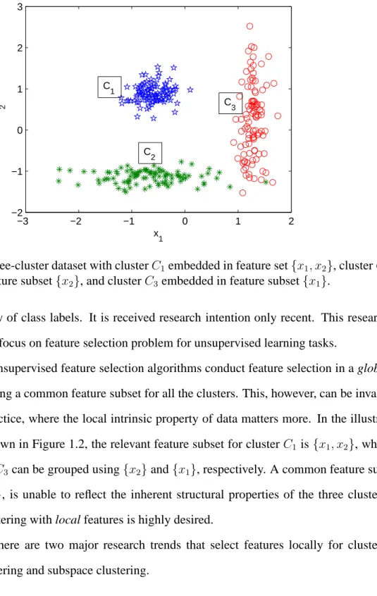
−3 −2 −1 0 1 2 −2 −1 0 1 2 3 x 1 x 2 C 1 C 2 C 3
Figure 1.2: A three-cluster dataset with clusterC1 embedded in feature set{x1, x2}, clusterC2
embedded in feature subset{x2}, and clusterC3 embedded in feature subset{x1}.
the unavailability of class labels. It is received research intention only recent. This research dissertation will focus on feature selection problem for unsupervised learning tasks.
In general, unsupervised feature selection algorithms conduct feature selection in a global sense by producing a common feature subset for all the clusters. This, however, can be invalid in clustering practice, where the local intrinsic property of data matters more. In the
illustra-tive example shown in Figure 1.2, the relevant feature subset for clusterC1 is {x1, x2}, while
clustersC2 andC3can be grouped using{x2}and{x1}, respectively. A common feature
sub-set, i.e., {x1, x2}, is unable to reflect the inherent structural properties of the three clusters.
Apparently, clustering with local features is highly desired.
In general, there are two major research trends that select features locally for clusters, namely, co-clustering and subspace clustering.
1.6.1
Co-clustering
In a co-clustering problem, data is stored in contingency or co-occurrence matrix C. The
co-clustering process derives sub-matrices from the large data matrix by simultaneously clus-tering rows and columns of the data matrix. Optimal co-clusclus-tering is derived based on the one that leads to the largest mutual information between the clustered random variables [31]. A well studied problem of co-clustering in data mining has been that of documents and words. The goal is to cluster documents based on the common words that appear in them and to cluster words based on the common documents that they appear in [32–36]. Co-clustering algorithms attempt to partition the features exclusively. That means a feature can only belong to a par-ticular cluster. This property limits its application in general feature selection for clustering problems.
1.6.2
Subspace Clustering
Subspace clustering [37] is another extension of traditional clustering that seeks clusters in different subspaces within a dataset. Subspace clustering algorithms localize the search for relevant features such that clusters which exist in multiple, possibly overlapping subspaces are determined. Subspace clustering approaches usually search for possible feature subsets on which density regions may occur, then clusters are discovered in the different subspaces.
1.7
Overview
In this dissertation, we focus on the problem of localized feature selection for unsupervised learning. The rest of the thesis is organized as follows: In Chapter 2, we review related works in the literature. In Chapter 3, we propose an algorithm of localized feature selection for un-supervised learning by cross-projection method. In Chapter 4, a probabilistic model of feature saliency with Gaussian mixture is addressed. The feature selection with model detection is inte-grated into Maximal Likelihood (ML) learning scenario. We propose another algorithm which performs clustering, feature selection, and cluster number detection simultaneously with Vari-ational Learning in Chapter 5. The conclusions of this thesis and recommendations for future
CHAPTER 2
RELATED WORK IN UNSUPERVISED FEATURE
SELECTION
In Chapter 1, we described the importance of feature selection and presented an overall picture of different approaches for feature selection. This chapter continues the discussion of unsupervised feature selection. We shall survey some of the recent feature selection algo-rithms. Since we are mostly interested in unsupervised learning, supervised feature selection algorithms are omitted from this survey. We organize the algorithms based on the scope of the feature subset (Global/Local), and the type of evaluation criteria (Filter/Wrapper).
2.1
Global Feature Selection
Feature selection algorithms generally process all clusters in a common subset. In other
words, an irrelevant feature fm is irrelevant to all clusters, and a relevant feature fn implies
that it is relevant to all clusters. The feature selection algorithm does not distinguish the dif-ferent response of a specified feature on difdif-ferent clusters. The output model is simple and straightforward.
2.1.1
Filters
A filter approach evaluates the quality of a feature subset without involving a particular clustering algorithm. It usually adopts a independent criterion, such as the feature similarity measure, or information measure, and finds the best subset through a search strategy.
The most well-known measure of similarity between two random variablesxand yis the
correlation coefficient, which is defined as
ρ(x, y) = p cov(x, y)
var(x)var(y)
(2.1)
vari-ables. Ifxandyare completely correlated, i.e., exact linear dependency exist,ρ(x, y)is 1 or
−1. If x and y are totally uncorrelated,ρ(x, y)is 0. Hence,1−|ρ(x, y)|can be used as measure
of similarity between two variables. This measure is used as a criterion in [17,38]. The reduced subset is obtained by discarding correlated features with a stepwise clustering scheme.
Correlation coefficient is invariant to scaling and sensitive to rotation, which are not de-sirable in many feature selection cases. Mitra et al. [17] suggest another linear dependency
measure, Maximal Information Compression Index (MIC) (λ2), for feature selection. MIC is
defined as follows
2λ2(x, y) =var(x) +var(y)−
q
var(x) +var(y)2−4var(x)var(y) 1−ρ(x, y)2
(2.2)
The value ofλ2 is zero when the features are linearly dependent and increases as the amount
of dependency decreases. Actually,λ2is equal to the eigenvalue for the direction normal to the
principal component direction of feature pair(x, y). It is also equal to the sum of the squares of
the perpendicular distances of the points(x, y)to the best fit liney= ˆa+ˆbx[39]. Based on the
feature similarity measure, the correlated features can be removed by some particular search strategy, such as Branch and Bound Search [40], Sequential Forward Search [40], Sequential Floating Forward Search [41], Stepwise Clustering [38]. In [17], features are partitioned into a
number of homogeneous subsets based on thek-nearest-neighbor (KNN) principle using MIC.
Among them the features having the most compact subset is selected, and its k neighboring
features are discarded. The best feature subset is generated by repeating this process until all of the features are either selected or discarded.
The above feature similarity measures are efficient to detect correlated features. However, they cannot detect irrelevant features. To overcome this issue, Dash et al. [26] proposed a
distance-based entropy measure, which is defined as, E =−X Xi X Xj DijlogDij + (1−Dij) log(1−Dij) (2.3)
whereDij is the normalized distance in the range[0.0, 1.0]. This method assigns a low entropy
to intra- and inter-cluster distances, and assigns a higher entropy to noisy distances. This
measure suffers from two drawbacks. (a) The mean distance of 0.5, the meeting point (µ) of
the left and right side of the entropy plot can be an inter-cluster distance, but still it is assigned the highest entropy. (b) Entropy increases rapidly for very small distances thus assigning very different entropy values for intra-cluster distances. An improved version is proposed in [16] as follows, E =X Xi X Xj Eij (2.4) Eij = exp(β∗Dij) exp(0) exp(β∗µ) exp(0) 0≤Dij ≤µ exp(β∗(1.0Dij))∗exp(0) exp(β∗(1.0µ)) exp(0) µ≤Dij ≤1.0 (2.5)
where Eij is normalized to the range [0.0, 1.0]. The parameter β, which is set based on the
domain knowledge, controls the entropy contribution of between intra- and inter-distances.
The parameter µ, which is updated heuristically, shifts the meeting point of the two sides of
the entropy-distance plot. The entropy of a particular feature is calculated by removing it from the original feature set and computing the entropy change thereby. Features are ranked based on their entropy. Best feature subset is obtained by selecting the top ranked features.
2.1.2
Wrappers
Filter feature selection approaches can be used by any clustering algorithms. However, the output is often not optimized for a particular clustering algorithm. On the other hand, a wrap-per approach utilizes a particular clustering algorithm to evaluate the wrap-performance of feature
subsets, thus usually produces better feature subset than a filter does. Most unsupervised fea-ture selection algorithms are wrappers. In this section, we review some wrapper approaches proposed very recent.
2.1.2.1
Cross-Projection
The quality of clusters can be measured by the within-cluster scatter matrix (Sw) and the
between-cluster scatter matrix (Sb),
Sw = k X j=1 πjE (X−µj)(X−µj)T|ωj = k X j=1 πjΣj (2.6) Sb = k X j=1 πj(µj−Mo)(µj−Mo)T, (2.7) Mo =E{X}= k X j=1 πjµj (2.8)
whereπj is the probability that an instance belongs to clusterωj,Xis ad-dimensional random
feature vector representing the data, k the number of clusters, µj is the sample mean vector
of cluster ωj, Mo is the total sample mean, Σj is the sample covariance matrix of cluster ωj,
andE{·}is the expected value operator. Many separability measures can be obtained based on
scatter matrix [42]. Among them,trace(S−1
w Sb)is widely used in literature [43]. However, this
criterion is biased on dimensionality, which means that the measure monotonically increases with dimension, assuming the clustering assignments remain the same. In order to elevate this
bias, Dy et al. [21] proposed a cross-projection method. Given two feature subsetsS1 andS2,
the clustering results areC1 andC2, respectively. LetCRIT(Si, Cj)be the clustering criteria
using feature subsetSi to represent the data andCj as the clustering assignment. The criteria
values for(S1, C1)and(S2, C2)are normalized as,
normalizedV alue(S1, C1) =CRIT(S1, C1)×CRIT(S2, C1) (2.9)
This cross-projection method ensures that the bias of dimensionality is removed, thus it can be used to compare the clustering quality on two different feature subsets, even though they may have different dimension. In [21], sequential forward search method is used to navigate through possible subset candidates. The number of clusters is estimated by merging clusters one at a time and using a Bayesian Information Criterion (BIC).
2.1.2.2
Law’s E-M Approach
Traditional feature selection algorithms have to search through the possible candidate sub-sets, which demands heavy computational load, even by greedy search methods. Law et al. [1] proposed another approach, which selects salient features and estimates the number of clusters simultaneously by Expectation Maximization (EM) algorithm. Assuming that the features are independent given a mixture component, and following a common distribution up to a prob-ability, the complement of this probability is defined as feature saliency and estimated by the Maximum Likelihood (ML) or Maximum A priori (MAP) with EM algorithm using Gaussian mixture models. The likelihood of such model is defined as follows,
p(y|θ) = k X j=1 αj d Y l=1 ρlp(yl|θjl) + (1−ρl)q(yl|λl) (2.11)
wherep(·)represents a probability distribution of a component,q(·)representing the common
distribution, θjl and λl denoting the parameters, ρl indicating the saliency of the particular
feature, and θ = {αj},{θjl},{λl},{ρl} . The model selection (estimating the number of
clusters) can be accomplished based on minimum message length (MML) criterion [44, 45]. The algorithm tries to minimize the following cost function,
−logp(Y|θ) + k+d 2 logn+ r 2 d X l=1 k X j=1 log(nαjρj) + s 2 X log(n(1−ρl)), (2.12)
wherer and sare the number of parameters inθjl andλl, respectively. This cost function is
selection with clustering simultaneously, and avoids the navigation over the possible feature subset candidates which is usually very large.
2.1.2.3
Variational Approach
[13] and [46] employ the same Gaussian mixture model as in [1] to describe feature rele-vance, but integrate model and feature selection under Bayesian framework. The model param-eters follow particular distributions instead of fixed values as estimated by EM algorithm. The learning process is to fit the distributions based on the given dataset. [13, 46] utilize variational learning techniques to estimate the underlying model. Since the cluster number also follows a distribution, it can be conducted directly.
2.2
Localized Feature Selection
Feature selection algorithms aforementioned are global, which means that the feature sub-set selected is common to all the clusters. However, in many applications, the natural grouping structure of a cluster is localized in a particular subspace, which implies that different clus-ters may have different relevant feature subset. The output format of such an algorithm is
{Ck, Fk}, where Ck and Fk indicate the cluster assignment and feature subset for a specific
clusterk. Notice that clustering results is required by those algorithms, thus localized feature
selection approaches are wrappers. Co-clustering and subspace clustering are two categories in this research area.
2.2.1
Co-clustering
Co-clustering (also called Biclustering, Bipartite, or two-mode clustering), is simultane-ous clustering of both instances and features such that the blocks induced by the row/column partitions are good clusters.
2.2.1.1
Information-Theoretic Co-Clustering
Let X and Y be discrete random variables that take values in the sets {x1, . . . , xm} and
Y. Co-clustering tries to find mapsCX andCY,
CX :{x1, x2, . . . , xm} → {xˆ1,xˆ2, . . . ,xˆk} (2.13) CY :{y1, y2, . . . , yn} → {yˆ1,yˆ2, . . . ,yˆl} (2.14)
which minimizes the following criterion,
I(X;Y)−I( ˆX; ˆY) (2.15)
whereI(X;Y) is the mutual information betweenX andY. Dhillon et al. [31] address that
the loss in mutual information can be expressed as,
I(X;Y)−I( ˆX; ˆY) =Dp(X, Y,X,ˆ Yˆ)kq(X, Y,X,ˆ Yˆ) =X ˆ X X x:CX=ˆx p(x)D(p(Y|x)kq(Y|xˆ)) (2.16) =X ˆ Y X y:CY=ˆy p(y)D(p(X|y)kq(X|yˆ)) (2.17)
whereD(·k·)denotes the Kullback-Leibler (KL) divergence, andq(X, Y,X,ˆ Yˆ)is a
distribu-tion of the form:
q(x, y,x,ˆ yˆ) = p(ˆx,yˆ)p(x|xˆ)p(y|yˆ). (2.18)
Thus the cost function can be minimized by alternatively improving row clusters (Equation (2.16)) and column clusters (Equation (2.17)). Similar models can be found in [47, 48].
2.2.1.2
Graphic Theoretic Co-clustering
Given an undirected bipartite graph G = (M, R, E), where M and R are two sets of
is the weight of an edge appearing between a vertexri ∈ R and a vertexmj ∈ M. There are
no edges between vertices of the same group. The adjacency matrix of the bipartite graph is expressed as, M = 0 B BT 0 (2.19)
The bipartite Laplacian matrix is defined as,
L= DR −B −BT D M (2.20)
where DR(i, i) = PjBij and DM(j, j) = PiBij. Co-clustering of the data is achieved by
partitioning the bipartite graph into two subsetV1 andV2. Shi and Malik applied spectral graph
partitioning to the problem of image segmentation in [49] by minimizing the objective function,
min x
TLx
xTDx (2.21)
wherexis a column vector such thatxi = c1 ifi ∈ V1 andxi = −c2 ifi ∈ V2. By relaxing
xi from discrete to continuous, it can be shown that the solution to (2.21) is the eigenvector
corresponding to the second smallest eigenvalue of the generalized eigenvalue problem [50,51],
Lx=λDx (2.22)
This eigenvalue problem can be reduced to a much more efficient Singular Value Decomposi-tion (SVD) [51] problem. Dhillon [52] and Zha et al., [53] employed this Spectral-SVD ap-proach to partition a bipartite graph of documents and words. Ding [54] performed document-word co-clustering by extending Hopfield networks [55][58] to partition bipartite graphs and showed that the solution is the principal component analysis (PCA) [2].
problems. However, in feature selection prospect, the feature subsets associated to different clusters are disjointed, which implies that a feature cannot be selected for several clusters. This restriction is often inflicted in general feature selection problems.
2.2.2
Subspace Clustering
Subspace clustering algorithms search for relevant features locally to find clusters that ex-ist in multiple, possibly overlapping subspaces. There are two major branches of subspace clustering based on their search strategy. Bottom-up approaches find dense regions in low di-mensional spaces and combine them to form clusters. Typical algorithms in this branch are CLIQUE, ENCLUS, MAFIA, Cell Based Clustering (CBF), CLTree, DOC, and SURFAING. Top-down algorithms find an initial clustering in the full set of dimensions and evaluate the subspaces of each cluster, iteratively improving the results. Typical top-down algorithms are COSA, PROCLUS, ORCLUS, and FINDIT.
2.2.2.1
CLIQUE
CLIQUE [56] combines density and grid based clustering to find low dimensional clusters embedded in high dimensional space. Each dimension is divided into bins using a static sized grid. Dense subspaces are sorted by coverage. The subspaces with the greatest coverage are kept and the rest are pruned. Adjacent dense grid units are discovered in each selected sub-space using a depth first search. Clusters are formed by combining these units using a greedy growth scheme. The hyper-rectangular clusters are then defined by a Disjunctive Normal Form (DNF) expression. Clusters may be found in the same, overlapping or disjoint subspaces. The clusters may also overlap each other. CLIQUE requires grid size and density threshold as input parameters. Tuning these parameters can be difficult.
2.2.2.2
ENCLUS
ENCLUS [57] is another subspace clustering method based heavily on the CLIQUE al-gorithm. The algorithm is based on the observation that a subspace with clusters typically has low entropy than a subspace without clusters. Thus ENCLUS computes the entropy
mea-sure rather than density and coverage (used in CLIQUE) to determine the clusterability of a subspace. ENCLUS also introduces interest, which is defined as the difference between the sum of entropy of measurements for a set of dimensions and the entropy of multi-dimension distribution, to measure the correlation of a subspace. Large values indicate higher correla-tion between dimensions. ENCLUS search for interesting subspace whose entropy exceeds a
thresholdωand interest gain exceedsǫ′. Clusters in the interesting subspaces can be identified
by the same methodology as CLIQUE. Parameters required by ENCLUS are grid interval∆,
entropy thresholdω, and interest thresholdǫ′.
2.2.2.3
MAFIA
CLIQUE and ENCLUS are sensitive to the uniform grid interval. MAFIA [58] introduces an adaptive grid based on the distribution of data to improve efficiency and cluster quality. MAFIA initially computes the histogram to determine the minimum number of bins for each feature. The adjacent cells of similar density are merged to form larger cells. In this man-ner, the dimension is divided into cells based on the data distribution and the resulting cluster parameters are captured more accurate. Once the bins have been defined, the clusterable sub-spaces are built up from on dimension as CLIQUE does. MAFIA requires the user to specify the density threshold and the threshold for merging adjacent windows. The running time grows exponentially with the number of dimensions in the clusters.
2.2.2.4
Cell-based Clustering Method (CBF)
The number of bins in many bottom-up algorithms increases dramatically as the number of features increases. To address this scalability issue, CBF [59] introduces a cell creation algo-rithm by splitting each dimension into a group of sections using a split index. The algoalgo-rithm creates optimal partitions by repeatedly examining minimum and maximum values on a given dimension which results in the generation of fewer bins. CBF requires two parameters,
sec-tion threshold which determines the bin frequency of a dimension, and cell threshold which
parameters.
2.2.2.5
CLTree
CLTree [60] uses a decision tree algorithm to partition each dimension into bins. It evalu-ates each dimension separately and then uses only those dimensions with areas of high density in further steps. To build CLTree, uniformly distributed noise data is added to the dataset, and the tree tries to split the real data from the noise. The density can be estimated for any given bin under investigation. After the tree is fully constructed, a pruning process is performed to obtain the final hyper-rectangle clusters. CLTree requires two parameters, min y which is the minimum number of points that a region must contain, and min rd which is the minimum relative density between two adjacent regions before the regions are merged to form a larger cluster.
2.2.2.6
DOC
Density-based Optimal projective Clustering (DOC) [61] is a hybrid method which blends the grid based bottom-up approaches and the iterative improvement method of the top-down
approaches. DOC attempts to discover projective clusters which are defined as pairs(C, D)
whereC is a subset of the instances andDis a subset of dimensions of the dataset, such that
C exhibits strong clustering tendency in D. The algorithm first selects a small subsetX by
random sampling. For a given cluster pair (C, D), instancep inC, and instanceq in X, the
following should hold true: for a dimensioniinD,|q(i)−p(i)| ≤w, wherewis the fixed side length of a subspace cluster or hyper-cube, given by the user. DOC also requires two additional
parameters,αthat specifies the minimum number of instances in a cluster, andβthat specifies
the balance between number of points and the number of dimensions in a cluster.
2.2.2.7
SURFING
SURFING (SUbspaces Relevant For clusterING) [62] computes all relevant subspaces and ranks them according to the interestingness of the hierarchical clustering structure they
distance). The algorithm first introduces a new variance measure that is half of the sum of
the difference of all objects to the mean value of k-nn-distance. The quality of the subspace
is defined by normalizing this variance to the production of mean value and the number of
objects having a smallerk-nn-distance than the mean value. SURFING evaluates subspaces
from one-dimension toldimension. At each iteration, irrelevant subspaces (whose quality
de-creases w.r.t its(l−1)-dimensional subspace below a threshold) are discarded. The remaining
l-dimensional subspaces are joined if they share any(l−1)dimensions. SURFING yields a list
of interesting subspaces ranked by their quality measure. Clusters existing in each subspace are further discovered by other clustering algorithms such as hierarchical clustering.
SURF-ING requiresk as the input parameter. The running time complexity isO(2dN2), though [62]
shows only a little percentage of subspaces are navigated in practice.
2.2.2.8
PROCLUS
PROCLUS [63] is a top-down subspace clustering algorithm. PROCLUS selectskmediods
from a sampled dataset. Those mediods are improved by randomly choosing new medoids and replacing the bad ones. Cluster quality is based on the average distance between instances and the nearest medoid. For each medoid, a set of dimensions is chosen whose average distances are small compared to statistical expectation. Once the subspaces have been selected for each medoid, points are assigned to medoids according to the average Manhattan segmental
dis-tance. Clusters with fewer than (N/k)× minDeviation points, where minDeviation is a
input parameter, are thrown out. Finally, the clusters and the associated dimensions are refined based to the points assigned to the medoids. PROCLUS also requires the average dimensional-ity of subspaces as an input parameter. The algorithm is sensitive to the parameters which are difficult to be determined in advance.
2.2.2.9
COSA
COSA (Clustering On Subsets of Attributes) [64] assigns weights to each dimension for each instance, instead of each cluster. The algorithm starts with equally weighted dimensions.
The weights are updated according to thek-nearest neighbors (knn) of each instance. Higher
weights are assigned to those dimensions that have a smaller dispersion within theknngroup.
New distances are calculated based on the updated weights. This process repeated until weights become stable. The neighborhoods for each instance are increasingly enriched with an instance belonging to its own cluster. The output is a COSA distance matrix based on weighted inverse exponential distance. Clusters are discovered by other distance based clustering algorithms such as hierarchical clustering. After clustering, the weight of each dimension for each cluster is computed based on that of its members. COSA does not need the number of dimensions
in clusters to be specified in advance. Instead, it requires a input parameter λ to control the
strength of intensive for clustering on more dimensions. Parameter k is also needed but the
author claims that the results are stable over a wide range ofkvalues.
2.3
Summary
Clustering is a fundamental technique in data mining and machine learning. Feature selec-tion is essential in many clustering problems, which helps the user focusing on the important attributes of data groups. Feature selection in unsupervised learning is much harder than that for supervised learning, due to the fact that the class labels, which are used to guide feature searching in supervised learning, are unavailable. Feature selection in unsupervised learning arises research intention only very recent. Most related works concentrate on global feature selection which select a common feature subset for all the clusters. Searching subsets for indi-vidual clusters is a new research area. Available localized feature selection algorithms can be found in co-clustering and subspace clustering. Co-clustering yields exclusive feature subsets for clusters, which is not suitable in many applications. Subspaces clustering algorithms en-countered difficulties such as heavy computational load, overlapping clusters, and/or requiring input parameters which are difficult to be determined in advance.
CHAPTER 3
NORMALIZED PROJECTION
In this chapter, we propose a heuristic localized feature selection algorithm for unsuper-vised learning. Our approach [65] computes adjusted and normalized scatter separability for individual clusters. A sequential backward search is then applied to find the optimal (perhaps local) feature subsets for individual clusters.
3.1
Introduction
Feature selection involves searching through various feature subsets, followed by the eval-uation of each of them using some evaleval-uation criteria [18–20, 30]. The most commonly used search strategies are greedy sequential searches through the feature space, either forward or backward. Different types of heuristics, such as sequential forward or backward searches, floating search, beam search, bidirectional search, and genetic search, have been suggested to navigate the possible feature subsets [11, 20, 41, 66]. In supervised learning, classification accuracy is widely used as evaluation criterion [19, 20, 30, 67, 68].
However in unsupervised learning, feature selection is more challenging since the class labels are unavailable to guide the search. Instead, clustering algorithms use some criteria, such as likelihood, entropy, or cluster separability measure to evaluate clustering quality and the feature subset quality. Regardless what the evaluation criteria are, global feature selection approaches compute them over the entire dataset. Thus, they can only find one relevant feature subset for all clusters. However, it is the local intrinsic properties of data that matter counts during clustering [69]. Such a global approach cannot identify individual clusters that exist in different feature subspaces. An algorithm that performs feature selection for each individual cluster separately is highly preferred.
The problem can best be illustrated using a synthetic dataset. We generate400 data points
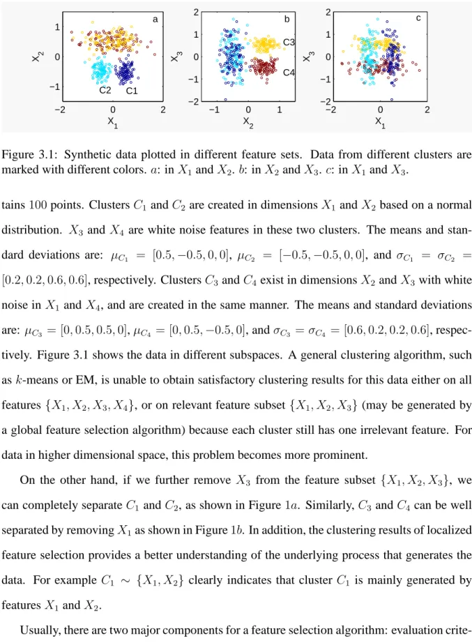
con-−2 0 2 −1 0 1 X 1 X 2 −1 0 1 −2 −1 0 1 2 X 2 X 3 −2 0 2 −2 −1 0 1 2 X 1 X 3 a b c C1 C2 C3 C4
Figure 3.1: Synthetic data plotted in different feature sets. Data from different clusters are marked with different colors.a: inX1andX2. b: inX2 andX3. c: inX1 andX3.
tains100points. ClustersC1 andC2 are created in dimensionsX1 andX2 based on a normal
distribution. X3 and X4 are white noise features in these two clusters. The means and
stan-dard deviations are: µC1 = [0.5,−0.5,0,0], µC2 = [−0.5,−0.5,0,0], and σC1 = σC2 =
[0.2,0.2,0.6,0.6], respectively. ClustersC3 andC4 exist in dimensionsX2andX3with white
noise inX1 andX4, and are created in the same manner. The means and standard deviations
are: µC3 = [0,0.5,0.5,0],µC4 = [0,0.5,−0.5,0], andσC3 =σC4 = [0.6,0.2,0.2,0.6],
respec-tively. Figure 3.1 shows the data in different subspaces. A general clustering algorithm, such
ask-means or EM, is unable to obtain satisfactory clustering results for this data either on all
features{X1, X2, X3, X4}, or on relevant feature subset{X1, X2, X3}(may be generated by a global feature selection algorithm) because each cluster still has one irrelevant feature. For data in higher dimensional space, this problem becomes more prominent.
On the other hand, if we further remove X3 from the feature subset {X1, X2, X3}, we
can completely separateC1 andC2, as shown in Figure1a. Similarly, C3 andC4 can be well
separated by removingX1as shown in Figure1b. In addition, the clustering results of localized
feature selection provides a better understanding of the underlying process that generates the
data. For example C1 ∼ {X1, X2} clearly indicates that cluster C1 is mainly generated by
featuresX1andX2.
Usually, there are two major components for a feature selection algorithm: evaluation crite-ria and feature subset search methods. In the following, we first discuss the evaluation criterion
for the localized feature selection algorithm, then the search method.
3.2
Evaluation Criteria
In this section, we first provide a brief introduction to scatter separability criterion, one of the well-known clustering criteria [21], and then show how this criterion could be adapted to localized feature selection.
LetSw andSb denote within-class scatter matrix and between-class scatter matrix,
respec-tively. We have, Sw = k X i=1 πiE{(X−µi)(X−µi)T|Ci}= k X i=1 πiΣi, (3.1) Sb = k X i=1 πj(µi−µ0)(µi−µ0)T, (3.2) µ0 =E{X}= k X i=1 πiµi, (3.3)
whereπi is the probability that an instance belongs to cluster Ci, X the d-dimensional input
dataset,k the number of clusters,µi the sample mean vector of clusterCi,µ0 the total sample
mean,Σi the sample covariance matrix of clusterCiandE{·}the expected value operator.
SinceSwmeasures how scattered the samples are from their cluster mean, andSbmeasures
how scattered the cluster means are from the total mean, the scatter separability is defined as
CRIT =tr(S−1
w Sb) (3.4)
Although there are a bunch of other separability criteria available, the measureCRIT enjoys
a nice property that it is invariant under any non-singular linear transformation [43]. However,
singular, the following separability criteria can be used instead,
CRIT =tr(Sb)/tr(Sw) (3.5)
In the remainder of this paper, we usetr(Sw−1Sb)in our discussion. However, one should be
aware thattr(Sb)/tr(Sw)is used for a singularSw.
Similar to the definition of Sw, we define S(
i)
w , the within-class matrix of an individual
clusterCias, Sw(i) = 1 ni E{(X−µi)(X−µi)T|Ci}= 1 ni Σi (3.6)
whereni is the number of points in clusterCi. Now we are ready to define the scatter
separa-bility of clusterCi.
Definition 1. The scatter separability of clusterCi is defined by,
CRIT(Ci) = tr(Sw(i)−1Sb) (3.7)
Assuming that identical clustering assignments are obtained when more features are added,
the scatter separabilityCRIT prefers higher dimensionality since the criterion value
mono-tonically increases as features are added [43]. The same conclusion could be drawn for the scatter separability for an individual cluster. Specifically, in [43], it is shown that a criterion
of the formXT
dSdXd, whereXdisd-column vector andSdis ad×dpositive definite matrix,
monotonically increases with dimension. Based on this, we have,
Proposition 1. CRIT(Ci)monotonically increases with dimensions as long as the clustering
Proof. SinceSb can be expressed asPkj=1ZjZjT whereZj is a column vector. CRIT(Ci) =tr(Sw(i)−1Sb) =tr(S(i)−1 w k X j=1 ZjZjT) = k X j=1 tr(Sw(i)−1ZjZjT) = k X j=1 tr(ZjTSw(i)−1Zj) = k X j=1 ZT j S (i)−1 w Zj (3.8)
Every term of Equation (3.8) monotonically increases with dimension, thus the criterion for an
individual clusterCRIT(Ci)monotonically increases with dimension.
To alleviate this problem, normalization of the separability criterion with respect to di-mensions is necessary for feature selection [21]. Moreover, for localized feature selection strategies, each cluster is associated with a distinct feature subset. It is usually impossible to
computeSb without proper normalization.
In the proposed algorithm, the normalization is performed using cross-projection over
in-dividual clusters. Suppose we have a cluster setC,
C ={(C1, S1), . . .(Ci, Si), . . . ,(Ck, Sk)} (3.9)
whereSi is the feature subset corresponding to clusterCi. To calculate the scatter separability
of(Ci, Si)in cluster set C, we project all the clusters ofC into feature subset Si, and extend
the scatter separability of clusterCi as follows,
by,
CRIT(Ci, Si)|C =tr(Sw(i)−1Sb)|C,Si (3.10)
where|C,Si denotes the project of cluster setC onto feature subsetSi.
Assume an iteration of search produces a new cluster setC′ on subspaceS′
i,
C′ ={(C1′, Si′), . . .(Ci′, Si′), . . . ,(Ck′, Si′)} (3.11)
Let’s also assume that cluster(C′
i, Si′)corresponds to cluster(Ci, Si), i.e.,(Ci′, Si′)is the cluster
that has the largest overlapping with(Ci, Si)in setC′. We then generate a new cluster set,C∗,
by replacing(Ci, Si)inCwith(Ci′, Si′),
C∗ ={(C1, S1), . . .(Ci′, Si′), . . . ,(Ck, Sk)} (3.12)
Note thatCRIT(Ci, Si)|C andCRIT(Ci′, Si′)|C∗ can not be compared directly because of the dimension bias. We have to cross-project them onto each other,
NV(Ci, Si)|C =CRIT(Ci, Si)|C ·CRIT(Ci, Si′)|C (3.13)
NV(Ci′, Si′)|C∗ =CRIT(Ci′, Si′)|C∗·CRIT(Ci′, Si)|C∗ (3.14)
After the cross-projection, the bias is eliminated and the normalized value NV can be used
to compare two clusters in different feature subspaces. A larger value of NV indicates larger
separability, i.e., better cluster structures.
3.2.1
Penalty of Overlapping and Unassigned Points
Localized feature selection implicitly creates overlapping and/or unassigned data points. Overlapping points are the data which belongs to more than one cluster, while unassigned
points are the data which belongs to non-cluster. Specifically, the overlapping measureO can be computed as, O = k X i6=j |Ci∩Cj| mean(|Ci|,|Cj|) (3.15)
whereCiandCj are two different clusters. And unassigned measureU can be computed as,
U = nu
n (3.16)
wherenandnuare the total number of data and the number of unassigned points, respectively.
Overlapping and/or unassigned data are allowed in some applications, and may be forbidden by other applications. Depending on the domain knowledge, we could adjust the impact of overlapping and unassigned points by introducing a penalty and obtain the adjusted normalized
valueANV.
Definition 3. The adjusted and normalized scatter separability pair of clusterCi in cluster set Con feature subsetSiand clusterCi′in cluster setC∗ on feature subsetSi′ is given by,
ANV(Ci, Si)|C =NV(Ci, Si)|C ·e(−α∆O−β∆U) (3.17)
ANV(Ci′, Si′)|C∗ =NV(Ci′, Si′)|C∗·e(α∆O+β∆U) (3.18)
where∆O and∆U are the changes on the overlapping and unassigned measure, respectively, if cluster(Ci, Si)is replaced by cluster(Ci′, Si′). αandβare two constants.
In Definition3,αandβare used to control the sensitivity with respect to overlapping points
and unassigned points. Large values ofαandβdiscourage the occurrence of overlapping and
unassigned data. On the other hand, ifαorβis zero, the corresponding effect of overlapping or
unassigned data will be ignored when comparing two clusters. The values forαandβdepend
of data is unassigned after clustering,β needs to be increased.
When two clusters(Ci, Si)and(Ci′, Si′)are compared, ifANV(Ci, Si)|C > ANV(Ci′, Si′))|C∗, we choose(Ci, Si). IfANV(Ci, Si)|C =ANV(Ci′, Si′))|C∗, we prefer the cluster in the lower
dimensional space. In addition, when two identical clusters are obtained in two different
fea-ture subsets, they have equal adjusted normalized valueANV, which is exactly what we want.
More formally,
Proposition 2. Given two identical clustersC1 =C2, and the corresponding feature subspaces
S1andS2, the adjusted normalized valueANV(C1, S1) = ANV(C2, S2).
Proof. SinceC1 =C2, we haveC=C∗. Thus
NV(C1, S1) =CRIT(C1, S1)·CRIT(C1, S2) =CRIT(C2, S2)·CRIT(C2, S1) =NV(C2, S2) And∆O = ∆U = 0. Thus ANV(C1, S1) =ANV(C2, S2) (3.19)
3.2.2
Unassigned/New data
In case some new data is obtained or unassigned data is not allowed by an application, assignments have to be made after clustering for these new/unassigned points. The
similar-ity of an instance and a cluster could be measured by either distance (k-means clustering), or
likelihood (EM algorithm). The additional difficulty introduced by localized feature selection algorithm is that clusters are associated with different feature subsets, making the direct com-parison among clusters meaningless. For distance based similarity, a straightforward solution is
to normalize the distance measure over its variance within each cluster, and assign the instance to a cluster that minimizes the normalized distance,
argmin Cj d=argmin Cj (kXi|Sj−µjk σ2 j ) (3.20)
whereXiis an unassigned point,µj the cluster mean vector ofCj,Sj the feature subset ofCj,
Xi|Sj the projection ofXiintoSj, andk · kis the norm of a vector. A similar method could be
developed for likelihood based similarity measure.
3.3
Search Methods
The cross-projection normalization scheme assumes that the clusters to be compared should be consistent in the structure of the feature space [21]. Consequently, we select sequential backward search instead of the sequential forward search adopted in [21]. The trade off is the slower clustering speed.
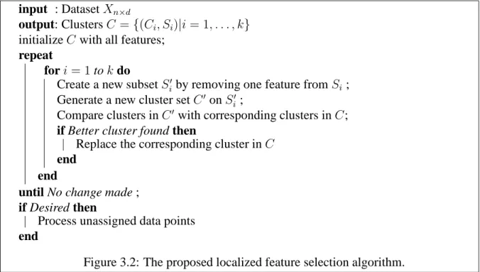
Specifically, the data are first clustered based on all available features. Then, for each clus-ter, the algorithm determines if there exists a redundant or noisy feature based on the adjusted
normalized valueANV defined in Equations (3.17) and (3.18). If so, it will be removed. The
above process is repeated iteratively on all clusters until no change is made, at which time the clusters with the associated feature subsets will be returned. The sequence of steps shown in Figure 3.2 illustrates our algorithm in detail.
The complexity is O(ndik) for the conventional k-means algorithm, and O(nd2ik) for
the GFS-k-means algorithm, respectively, where n is the number of points, d the number of
features,ithe number of iteration (usually unknown), and kthe number of clusters. The
com-plexity of our approach, in worst case, isO(nd3k2i)with backward sequential search. It shows
that for data sets with very high dimensions and large number of clusters, the proposed
algo-rithm is slow compared to generalk-means and global feature selecting algorithms. However
input : DatasetXn×d
output: ClustersC ={(Ci, Si)|i= 1, . . . , k}
initializeCwith all features;
repeat
fori= 1tok do
Create a new subsetS′
i by removing one feature fromSi;
Generate a new cluster setC′ onS′
i ;
Compare clusters inC′ with corresponding clusters inC;
if Better cluster found then
Replace the corresponding cluster inC
end end
until No change made ; if Desired then
Process unassigned data points
end
Figure 3.2: The proposed localized feature selection algorithm.
3.4
Experiment and Results
We evaluate the localized feature selection algorithm using both synthetic and real-world
datasets. The experiment results are obtained by choosingk-means as the clustering algorithm.
However, note that the adjusted normalized valueANV is not restricted tok-means. It can be
used together with any general clustering algorithm.
In general, it is difficult to evaluate the performance of a clustering algorithm on high dimensional data. Localized feature selection presents an additional layer of complexity by associating clusters to different feature subsets. Therefore, we take a gradual approach for our evaluation. We first test the proposed algorithm on a small synthetic dataset with known data distribution along each feature dimension. Then, we investigate five real-world datasets downloaded from UCI repository [70]. On all UCI datasets, we perform a semi-supervised learning strategy for evaluation purpose. This makes it possible for us to compute a pseudo-accuracy measure for easy comparison among different algorithms. However, one should be aware that the “true” class labels are not always consistent with the nature grouping of the underlying dataset. Thus, the quality of clusters should be further analyzed in addition to the
pseudo-accuracy. For this purpose, we also illustrate our results by visually examining the clusters in the selected feature subspace on synthetic data and Iris data.
On each dataset, we compare our localized feature selection algorithm (withk-means,
de-noted by LFS-k-means) with global feature selection algorithm (also withk-means, denoted
by GFS-k-means), and k-means without feature selection. GFS-k-means is implemented in a
similar fashion as [21]. The only difference is that we adopted the backward search strategy
due to the reason discussed in Section2.3.
On the above experiments, the number of clustersk is set to the “true” number of classes.
This is not always applicable in real world applications. How to determine the value ofk is a
common problem in unsupervised learning. It may strongly interact with the predicted clus-ter structures, as well as the selected feature subset in feature selection algorithms [1]. There
are several algorithms available to determine k, i.e., [1, 43, 71]. Another common problem
that a clustering algorithm usually faces is how to initialize cluster centroids. Bad initial clus-ters/centroids might lead to low quality clusters. In traditional clustering algorithms, some
techniques, such as randomly picking up k patterns over the dataset, preliminary clustering,
or choosing the best from several iterations, are frequently used to alleviate the chance of bad initial clusters. In our approach, bad initial clusters for backward searching may occur more often when many noise features presented, and might affect the final clusters and feature sub-sets largely. This problem can be alleviated by preliminary clustering with a global feature selection, i.e., [1].
We incorporate another experiment as an example solution for unknownkand preliminary
clustering in Section 3.4.4. In this section, we evaluate our algorithm over another three UCI
datasets with unknownk. We first employ the algorithm proposed in [1] to estimate the
num-ber of clusters, global feature saliencies and cluster centroids. Then we use them as initial parameters and run our algorithm on the particular dataset. Clusters obtained are labeled to its majority portion of true classes. Errors are calculated accordingly.
Table 3.1: Confusion matrix and error rate on the synthetic data. C1 - C4 are the output cluster labels, and T1 - T4 are the true cluster labels
Algo k-means k-means w/oX4 GFS-k-means LFS-k-means
Label C1 C2 C3 C4 C1 C2 C3 C4 C1 C2 C3 C4 C1 C2 C3 C4 T1 77 22 1 0 59 40 1 0 37 17 46 0 99 0 0 1 T2 3 76 0 21 45 49 0 6 33 22 45 0 0 100 0 0 T3 1 7 89 3 0 3 69 28 26 16 58 0 0 1 98 1 T4 23 0 9 68 3 0 45 52 35 14 51 0 2 0 0 99 Error 0.225 0.428 0.708 0.01
Table 3.2: Feature subset distribution on the synthetic data. C1 - C4 are the output cluster labels. Feature Subset(s) Algorithm C1 C2 C3 C4 k-means {1, 2, 3, 4} GFS-k-means {4} LFS-k-means {1, 2} {1, 2} {2, 3} {2, 3}
3.4.1
Synthetic data
The synthetic data is described in Section 3.1 and illustrated in Figure 3.1. Penalties of
overlapping and unassigned points (αandβ) are set at1.
Table 3.1 shows the confusion matrix and error rate of k-means with full feature set, k
-means without the totally irrelevant feature X4, GFS-k-means, and LFS-k-means, and
Ta-ble 3.2 shows the selected feature subsets. Clearly, by employing all four availaTa-ble features,
k-means performs poorly with a error rate of 0.225, which indicates that irrelevant features
greatly reduce the clustering performance. Meanwhile, GFS-k-means does a terrible job with
an unacceptable error rate of0.708. The output feature subset contains only the noisy feature
X4! This surprising result could be explained as follows. Since each feature is irrelevant to at
least two clusters and each cluster has at least two irrelevant features, NO feature subset are
relevant to all clusters. We also evaluatedk-means algorithm on the feature subsetX1, X2, X3,
Table 3.3: Confusion matrix and error rate on iris data. C1 - C3 are the output cluster labels, and T1 - T3 are the true cluster labels
Algo k-means GFS-k-means LFS-k-means
Label C1 C2 C3 C1 C2 C3 C1 C2 C3
T1 50 0 0 50 0 0 50 0 0
T2 0 39 11 0 46 4 0 48 2
T3 0 14 36 0 3 47 0 4 46
Error 0.167 0.0467 0.04
Table 3.4: Feature subset distribution on iris data. C1-C3 are the output cluster labels. Feature Subset(s)
Algorithm C1 C2 C3
k-means {1, 2, 3, 4}
GFS-k-means {3}
LFS-k-means {4} {3, 4} {3, 4}
feature selection algorithm, as shown in Table 3.2. The error rate is as high as 0.428, indi-cating that the group structures can not be recognized with globally relevant feature subset.
The reason is that the structures are buried not only by the irrelevant feature X4, but also by
the relevant features X1 andX3. On the other hand, the proposed localized feature selection
algorithm produces an excellent result with a error rate of0.01. From Table 3.2, we can see
clearly that the relevant features for each cluster are selected correctly, and the clusters are well separated in the corresponding feature subspaces (Figures 1a and 1b). This result confirms that selecting features locally is meaningful and necessary in clustering.
3.4.2
Iris data
Iris data from UCI is a widely used machine learning benchmark dataset for both
super-vised learning and unsupersuper-vised learning. This data has three classes, four features, and 150
instances. In this experiment, we setαandβto be1and6, respectively.
Table 3.3 shows the confusion matrix and error rate of k-means, GFS-k-means, and
4 5 6 7 8 2 2.5 3 3.5 4 X 1 X 2 2 4 6 0 0.5 1 1.5 2 2.5 X 3 X 4 C1 C2 C3
Figure 3.3: Scatterplots on iris data using features 1 and 2 (left panel), and using features 3 and 4 (right panel). Data from different classes are marked with different colors.
all four features, is able to successfully identify cluster 1, “iris-setosa”. However it does not
perform well on cluster 2, “iris-versicolor”, with a error rate of 0.22, and cluster 3,
“iris-virginica”, with a error of0.28. The GFS-k-means discards feature1,2, and4, and recognizes
the structure


![Table 3.6: UCI datasets with estimated number of clusters and initial centroids. GFS: Global feature selection and clustering by algorithm of [1]](https://thumb-us.123doks.com/thumbv2/123dok_us/381929.2542258/48.918.139.817.115.1056/datasets-estimated-clusters-initial-centroids-selection-clustering-algorithm.webp)