Forecasting Sales

Forecasting Sales

Philip Hans Franses Econometric Institute Erasmus University Rotterdam

Econometric Institute Report 2009-29

Abstract

This chapter deals with forecasting sales (in units or money), where an explicit distinction is made between sales of durable goods (computers, cars, books) and sales of utilitarian products (SKU level in supermarkets). Invariably, sales forecasting amounts to a combination of statistical modeling and an expert’s touch. Models for durable goods sales are usually based on (variants of) the Bass model, while SKU sales forecasts are typically based on simple extrapolation methods. Forecast evaluation is not standard due to the interaction of model and expert.

Key words: Sales forecasting; durable goods; SKU-level sales; diffusion; human judgment

This version: September 24 2009

Author’s notes: This chapter is prepared for the Oxford Handbook on Economic Forecasting, edited by Michael Clements and David Hendry. Thanks are due to Richard Paap and Dick van Dijk for helpful comments and experts at Philips Electronics (Amsterdam) and Organon BV (Oss) for their help with the data. Address for correspondence is Econometric Institute, Erasmus School of Economics, PO Box 1738,

1. Introduction

Sales forecasts are important for inventory management and for marketing. Inventories can be kept at appropriate levels, and marketing efforts can be addressed in case sales projections do not meet a firm’s aspirations. Many firms keep detailed records of sales levels, usually at a high frequency level. It is common to have readily access to daily and weekly sales levels in retail stores, while sales of durable products like cars, refrigerators and television sets (but also such sales as concerning airline passengers) are usually recorded monthly. This chapter deals with forecasting methods for durable (some of these could be called hedonic) products, like HD television and hybrid cars, and methods for stock-keeping unit (SKU) products we regularly purchase, like food products.

The main theme of this chapter is that sales forecasts for these products are rarely based on statistical models only. Typically, the starting point is such a statistical model, but in the end a manager or expert gives the forecasts a final twist. For durable products this is due to the fact that one usually needs to have some impression of the expected total sales (to be achieved perhaps many years in the future). This guesstimate is usually given by the responsible product manager, and over time it gets modified. The model that is often used for forecasting durables’ sales can only estimate total sales (with some degree of accuracy) when sales is very close to total sales, that is, by the time its forecast in not of interest anymore. For SKU level products, forecasts are usually created by extrapolation methods (packaged in specialized software so that quick updates can be made). As managers usually know this, they adapt the forecasts towards their expectations, or sometimes even ignore the model forecasts altogether. The combination of models with experts has an important consequence for the evaluation of forecasts, as will be reviewed below.

This chapter starts with a section on durable products. The typical model that is used for forecasting is the Bass (1969) model, or one of its many variants. This model has various pleasant features, and it is usually well understood by managers, which is quite relevant in this area of sales forecasting. The Bass model can be extended to capture sales of sequential generations, and also multi-level versions are available. This section will review various recent developments concerning the Bass model.

Section 3 deals with forecasting SKU level sales data. Due to the very fact that such forecasts have to be made on a frequent basis and also for many products at the same time, it is quite common to have automated programs generate forecasts and to have managers give these forecasts a final twist. Recently, this practice has become topic of much research, which is due to the fact that detailed databases have become available. A review of the findings in this literature is given.

The final section gives a summary of the current state of the art. Also, it gives a few further research topics.

2. Durable products

Consider a variable that measures sales of durable product. Usually, the pre-sample observations are equal to zero as then the product was not yet available. At one moment sales start to increase, then they reach a peak, and eventually sales die out to zero. This pattern implies the familiar S-shape for cumulative sales. Cumulative sales level off to the so-called maturity level usually labeled as m.

The Bass model, in theory

The Bass (1969) theory starts with a population of m potential adopters. For each of these adopters, the time to adoption is a random variable with a distribution function F() and density f(), such that the hazard rate satisfies

(1) ( ) ) ( 1 ) ( _   qF p F f   

where τ refers to continuous time. The parameters pand qare associated with innovation and imitation, respectively. The cumulative number of adopters at time , denoted asN(), is a random variable with mean

(2) N()E[N()]mF().

The function N() satisfies the differential equation

(3) ( ) ( ) [ ()] ()[ ()].    N m N m q N m p d N d n     

The solution of this differential equation for cumulative adoption is

(4)              _ __  (₍ )₎ 1 1 ) ( ) ( _{p q} p q q p e e m mF N ,

and for adoption itself it is

(5) _          _2_{( }(₎ ₂) ) ( ) ( ) ( ) ( _    _{p q}p q qe p e q p p m mf n .

Analyzing these two functions of  reveals that N() indeed has a sigmoid pattern, and hence that n()has a hump-shaped pattern.

The Bass model for actually observed data

The above expressions are all in continuous time. In practice one of course has discretely observed data, like per year or per quarter. DenoteXtas the adoptions and denoteNt as

the cumulative adoptions, where t corresponds with the discretely observed data. There are now various ways to translate the continuous time models above into models that can be fitted toX_t and/orN_t.

(6) t t t t t t t t t t t N N N m q N p q pm N m N m q N m p X                            2 1 3 1 2 1 2 1 1 1 1 1 ) ( ) ( ) (

where it is assumed that _t is an independent and identically distributed error term with mean zero and common variance _2_{. Bass (1969) proposes to use ordinary least squares} [OLS] to estimate the parameters in (6), where non-linear least squares [NLS] is needed to estimate the standard errors of pˆ , qˆ and mˆ . Of course, for forecasting only estimation results for ˆ₁, ˆ₂ and ˆ₃ are required and just OLS can be used.

To add an error term to an equation like (3) is one of the possible ways to match the theoretical Bass model with the data, see also Putsis and Srinivasan (2000). Recently, Boswijk and Franses (2005) have proposed an alternative to the expression in (6). It is based on the notion that N() can be viewed as an equilibrium path around which the actual cumulative adoptions may fluctuate. They assume that the stochastic features of the diffusion process originate from the tendency of the data to revert to that equilibrium path in an error-correction-type of way. The model to be fitted to actual data would become

(7) X_t ₁₂N_t1₃N_t2_1₄X_t1_t

Boswijk and Franses (2005) also propose to make the error process heteroskedastic, such that uncertainty around the diffusion path is largest around the sales peak. Interestingly, (7) differs from (6) with the repressorsXt_1.

Another empirical version of the Bass diffusion theory, which is often used in practice due to its convenience, is proposed in Srinivasan and Mason (1986). These authors argue that aggregation bias may occur if one moves from (3) to (6). Therefore, they propose to apply NLS to

(8) Xt m[Ft(p,q)Ft1(p,q)]t where (9)            _ _pqt p q t q p t e e q p F _{( )} ) ( 1 1 ) , (

Generating forecasts from the Bass model

The Bass model is used to forecast future sales and cumulative sales data. It is quite important to recognize that fitting and forecasting usually do not occur for the same data. This needs a few words of explanation. The most important moment to generate forecasts for sales is prior to the launch of the new product or just right after its launch. By then, there are usually not enough data to accurately estimate the key parameters. In fact, as van den Bulte and Lilien (1997) show, when the data did not yet pass the moment of peak sales, which is the point of inflection in the cumulative sales curve, only unreliable estimates of p and q can be obtained. In other words, by the time the parameters can properly be estimated, that is, some time after peak sales, one basically is not anymore interested in the forecasts.

Practical sales forecasting of durable products proceeds along other lines, see Lilien, et al. (2000) for a detailed account. First, one considers the (cumulative) sales patterns of products that are similar to the current one that is about to be launched. Given the availability of the relevant data of for example previous generations of the same product (like PlayStation3 and PlayStation2) or of data concerning countries where the same product has already been introduced, one obtains initial values of p and q. What is then still missing is an initial estimate of m. The value of the total number of adopters is usually set by the manager. It is based on experience with similar products in the past, with the same product in other countries and potentially based on marketing research involving conjoint measurement (that is, questionnaires where individuals can indicate whether they prefer certain new but by then still hypothetical products).

summarized, see for example Chandrasekaran and Tellis (2008), Talukdar et al. (2002) and Tellis et al. (2003) among many others. One can make the characteristics of the diffusion process, for example as summarized by the p and q parameters, a function of characteristics of countries.

To make point forecasts for sales one can use one of the above expressions, like in (6), (7) or (8). The model in (8) seems to imply the easiest way to construct forecasts. When t = n is the forecasting origin, and h is the horizon, one can simply use

(10) Xˆ_nh mˆ[F_nh(pˆ,qˆ)F_nh1(pˆ,qˆ)]

where p, q and m are set at values using the methods discussed above. When the error term is an ARMA type process, straightforward modifications of (10) can be made. If the error term has an expected value equal to 0, then the forecasts from (10) are unbiased for any horizon h.

Unbiased forecasts are not automatically obtained from the Bass model as given in (6) or (7), which is due to the fact that these equations involve the term 2

1 

t

N . The true one-step-ahead observation, based on (6), is

(11) 2 ₁ 3 2 1 1     n  n  n n N N X    

and the forecast from origin n is then

(12) 2 3 2 1 1 ˆ ˆ ˆ ˆ n n n N N X _   

and the squared forecast error is _2_{. This one-step-ahead forecast is unbiased.} For two steps ahead, matters become different. The true observation is

(13) 2 ₂ 1 3 1 2 1 2       n  n  n n N N X    

which, as Nn_1 Nn Xn_1, equals (14) 2 ₂ 1 3 1 2 1 2 (  ) (  )     n  n  n  n  n n X N X N X    

Upon substitutingX_n1, this becomes

(15) 2 2 1 2 3 2 1 3 1 2 3 2 1 2 1 2 ) ( ) (                 n n n n n n n n n n N N N N N N X            

If (15) is used to generate Xˆn_2 by incorporating the known observations at time n, then

the two-step-ahead forecast error is based on

(16) ] 2 ) 1 ( 2 2 [ ˆ 2 1 1 2 3 1 2 1 1 3 1 2 2 2 2                 n n n n n n n n n n N N X X           

From (16) one can derive that the expected forecast error is

(17) 2 3 2 2 ˆ ) (Xn_ Xn_   E

For h = 3 and beyond, this bias grows exponentially. The size of the bias depends on the parameters ₃ and_2_{. As 0}

3 

 , the forecast Xˆ_n2 that follows from (15) is upward biased.

To obtain unbiased forecasts for the Bass regression models for h = 2, 3,…, one needs to resort to simulation techniques. Consider again the Bass regression model, where it is now written as

where Z_t1 contains 1, N_t1 and N_t2_1 and contains p, q and m. A simulation-based one-step-ahead forecast is now given by

(19) Xˆn1,i  g(Zn;ˆ)i

where e_i is a draw from the N(0,ˆ2)distribution. Based on I such draws, an unbiased forecast can be constructed as

(20)



This simulation approach gives the full distribution of forecasts. A two-step simulation-based forecasts is simulation-based on the average value of

(21) Xˆ_n2,i  g(Z_n,X_n1,i;ˆ)_i

again for I draws.

An empirical illustration

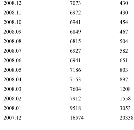
To illustrate the Bass model, consider the data as they are displayed in Figure 1, which concern sales of LCD television sets 15 inch for 2004 February to and including December 2008. Estimating the parameters using NLS for the representation as in (7) gives the estimates mˆ 7073 with standard error 430, pˆ 0.0019(0.0013) andqˆ 0.0465(0.0126). The parameter ₄ is estimated as 0.457 with standard error 0.121. These parameter estimates seem quite reliable, and the main reason for that is that peak sales seem to have occurred in the early months of 2008, which can also be observed from the cumulative sales data as they are presented in Figure 2 where the point of inflection is clearly visible.

The relevance of having passed the moment of peak sales is demonstrated using the numbers in Table 1. When the sample would have ended in the beginning of 2008, then estimates of m would haven very imprecise, that is, the standard errors are very large. Even more so, when the sample would have ended right before the inflection point, the estimate of m is highly unreliable.

Suppose now that the sample ends way before the inflection point, then one would need to fix the value of the maturity level in order to get proper estimates of the shape of the function. To demonstrate this, suppose the sample ends in November 2005, which is one month before the strong seasonal peak in December 2005. If an expert with domain knowledge would have set the m at 7100, then one gets pˆ 0.0032(0.0011)

andqˆ 0.0803(0.0290), which are estimates that are is reasonable in range with the

earlier presented full sample estimates. Hence, this suggests that the shape of the curve, which is characterized by the p and the q parameters can reasonably be predicted using a first guess of m.

As mentioned, early forecasts for the sales patterns of new products are usually based on the parameter estimates obtained for similar products. For example, consider the sales of LCD television sets of 20 inch, 5 inch more than the product considered in Figure 1 (and pretend this product is launched a long time after the earlier product). Suppose the p and q estimates for the Bass model for the 15 inch television sets are fixed, and suppose the sample ends in November 2005, then an estimate for m is found as 9527 (x 1000 units). For the full sample, the estimates are mˆ 8305 with standard error 239,

) 0011 . 0 ( 0027 . 0 ˆ 

p andqˆ0.0575(0.0135). The parameter ₄ is estimated as 0.411 with standard error 0.124. This shows that with the help of parameter estimates from a similar product, one can get reasonable estimates of the sales curve for the considered product.

In sum, an expert with domain knowledge can guesstimate the value of m and fit p and q reasonably early and well before the inflection point. Also, with p and q from elsewhere, one can estimate m reasonably well. In practice, one updates this procedure each time new information comes in, see Lilien et al. (2000) for a detailed account.

Forecasting the timing of peak sales

For many new products it is most important to forecast the moment of peak sales. If this moment is felt to come too early or too late, one can change marketing efforts and lower prices or increase distribution levels. The timing of peak sales can be derived from

(22) _        p q q p T* 1 log Denoting *

m as the amount of cumulative sales at that time, and writing

m m f  * , Franses (2003) derives that

(23) ) 1 ( 2 ) 2 1 log( ) 1 2 ( _* f T f f p     (24) ) 1 ( 2 ) 2 1 log( * f T f q    .

Imposing these expressions in (6) or (7) allows one to use NLS and to get immediate estimates and standard errors of *

T and f.

Three important extensions of the Bass model

The Bass model and its variants have been extended in various directions with notably three important ones that are often applied in practice. The first important extension concerns the sequence of generations of the same product, think of computers with more and better capacities and further editions of textbooks. Norton and Bass (1987) propose a model for successive generations, and it reads as follows. Suppose that there are two generations, and that the first generation is introduced at timet 0 and that the second

(25)            _{ p}_{q t} p q t q p t e e q p F _{( )} ) ( 1 1 , 1 _{1 1} 1 1 1 1 1 1 ) , ( and            _p_{q t} p q t q p t e e q p F _{( )} ) ( 2 2 , 2 _{2 2} 2 2 2 2 1 1 ) , ( ,

then the Norton and Bass (1987) model reads as

(26) _{1, 1,} ( ₁, ₁) ₁[1 _2, ( ₂, ₂)] 2 p q F m q p F S _t  _t  _t

for the sales of the first generation and

(27) _{2, 2,} ( ₂, ₂)[ _{2 1,} ( ₁, ₁) ₁]

2 p q m F p q m

F

S _t  _t  _t

for the sales of the second generation. In words it says that once the second generation is introduced, it eats away some of the potential sales of the first generation. When certain restrictions are imposed on p₂ andq₂, based on the values for the first generation, one can make early forecasts for the sales pattern of the second generation.

A second generalization of the Bass model amounts to adding a second level to the model. Consider the Bass model for the i-th product, that is

(28) _{it it} i i t i i i i i t i N m q N p q m p X _,  (  ) _,1  2_,1 _,

and assume a second level to this model in which the parameters are linked with variables that are constant over time and only vary across the products, that is,

(29) i i i i i i i i i w Z m v Z q u Z p       3 2 1   

A two-step estimation method is put forward in Talukdar et al. (2002), but this approach underestimates the uncertainty in the second level as it treat the estimates in the first

round, that is (28), as observable variables in model (29). In fact, the variables in (29) are estimates too, so a proper estimation method takes that into account. To this end, Fok and Franses (2005) propose a simulated maximum likelihood method. One of the important features of this two-level model is that forecasts for the p, q and m parameters can be made based on observable characteristics of the products or the countries in which they are sold.

The third often used extension of the Bass model is called the Generalized Bass model and it is put forward in Bass et al. (1994). The key idea of this model is to change (1) into (30) [ ( )][1 ( ) ( ) ...] ) ( 1 ) ( 2 2 1 1              x x qF p F f

where x₁()andx₂()are marketing mix variables. It is important to understand that the marketing mix variables preferably should enter the equation as step functions or growth rates. The key reason for that is outlined in Bass et al. (1994) and this is that when the marketing variables have a trend themselves or even an S-shape trend, then this implies that one can estimate a Bass model without the decision variables as then the model can be approximated by (31) [ ( )] ) ( 1 ) ( * * _   F q p F f    where *

p and q*mop up the effects of these additional variables.

In sum, the Bass model and its variants are regularly used in marketing practice and in academic articles. It is tractable and its parameters have an interpretation, it can be extended in various directions, and parameters are easy to estimate. In practice, the Bass model parameter estimates are always supported by an expert’s touch. This is simply because the model is typically used to forecast sales when the product has not yet been introduced. By the time sales levels reach maturity, there is no need to create forecasts, as

3. SKU-level sales

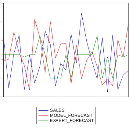
SKU-level sales data have properties that are very different from those of durable products and this inevitably leads to the use of different forecasting techniques. One of the features of SKU level data is that there are usually many of them. A regular retail store carries thousands of SKUs and may want to make forecasts on a weekly basis. Indeed, a second feature is that data are available at frequencies as high as daily. Managers want detailed forecasts so most SKU series are not aggregated. Third, SKU-level data some irregular patterns due to a variety of reasons, like holidays, out-of-stock conditions, price cuts, promotions and so on. Hence, SKU-level data are not easy to forecast. In Figure 3 a typical graph is given of monthly sales of a pharmaceutical product, and clearly, the pattern is quite erratic.

Statistical models

Marketing scholars often rely on variants of the so-called SCAN*PRO model originally proposed in Wittink et al. (1987). This model basically is a standard linear (log-log) regression model where it contains a variety of variables (sales, prices, promotions, distribution) and their interactions.

In everyday practice, however, people rarely fit fully parameterized econometric models, but rely on simple extrapolation techniques that are often encapsulated in professional forecasting software. Examples are ForecastPro™ and Autobox™. In the forecasting literature one regularly reviews this software and evaluates their newly added tools.

In the forecasting literature there is ample evidence that simple extrapolation techniques lead to the most accurate forecasts, more than more involved econometric regression models. A recent account of a large-sized forecasting competition is given in Makridakis and Hibon (2000), with statistical support in Koning, et al. (2005), and it is commonly found that, across many time series (thousands) with differing aggregation levels, with different amount of outliers and so on, it is Holt-Winters like methods and simple Box Jenkins time series models that are best on average. The professional

software usually has these routines included, amongst other extrapolation methods, and each time, parameters are updated and the best model is selected. Key aspect is that the input to these methods often simply is lagged sales data, and perhaps deterministic terms as linear or quadratic trends.

The fact that it is only lagged sales data that is included is crucial here. Most local experts or managers know that the forecasting software includes only lagged sales, and even though forecast competitions say that small models are best, most managers modify the model-based forecasts. There is a large literature of forecast adjustments (Armstrong and Collopy, 1998; Sanders and Manrodt, 1994; Sanders and Ritzman, 2001; Mathews and Diamantopoulos, 1986; Goodwin, 2000, 2002), but only recently substantial empirical evidence has been documented concerning SKU-level forecasts. Fildes and Goodwin (2007), Fildes et al. (2009) and Syntetos et al. (2009) document that expert adjustment occurs quite frequently and also that over-optimism of experts is found to cause adjustment to be more often upwards than downwards. Franses and Legerstee (2009a), while analyzing experts allocated in many countries making forecasts for pharmaceutical products within various distinct categories, find that expert adjustment itself is largely predictable and that expert adjustment is not independent from the model-based forecasts. Furthermore, Boulaksil and Franses (2009) interviewed these very same experts, and about half of them claim not to look at model forecasts at all when they make their own expert forecasts. This touches upon an important issue and that is that experts rarely document what it is that they do when creating their own forecasts.

The ideal expert touch

The question now is what these recent empirical results actually mean and also which impact they have on the empirical analysis of expert forecasts. Consider a SKU-level sales series variable St and suppose it can be described by a first-order autoregression,

like (31) ~ ( , 2) 1     t_ t N S S

where _2_{is the variance of the error term}

t

 , which is defined as the difference between

t

S and S_t1. The parameters can be estimated using OLS.

The one-step-ahead model-based forecast for the dependent variable that can be created from model (31) reads as

(32) M _t

t S

Sˆ_1 ˆˆ

The one-step-ahead forecast error is

(33) M _t

t

t S  S

ˆ_1  _1 ˆ ˆ ,

and it is this error that is crucial.

Suppose that there is an expert with domain knowledge, and who receives the model-based forecast (32). Suppose further that this expert is allowed to adjust this model-based forecast. To understand more of what an expert could optimally do, one needs a few assumptions. The first is that the model in (31) is properly specified. This means that the model contains the appropriate explanatory variables, that the parameters are estimated consistently, and that the errors are uncorrelated over time. Normality is not specifically required, as long as the distribution is symmetric and as long as there are not too many outliers. The second assumption is that the expert agrees that model (31) is properly specified. That is, the expert knows how the model works, how the variables were selected, and how the parameters were estimated. This seems to hold for many practical cases where statistical forecasting software is used. Given these assumptions, it is easy to conceive that somehow optimal expert adjustment of a model-based forecast as in (32) entails that the expert believes to know part of the forecast error (33). In other words, the experts believes that

where Wt_1contains various variables and where t1 is a time-varying parameter vector. The parameters in_t1 cannot be constant over time, as then the model would not have been correctly specified.

One might call Wt_1t_1 the intuition of the expert, as it is not replicable nor is it

predictable. Ideally, Wt_1t_1 has mean zero, and this makes the expert forecast unbiased,

like the model forecast, as the expert forecast is given by

(35) ˆE_1  ˆ ˆ _t  _{t1 t1}

t S W

S   

This expression also shows that the expert forecast nests the model-based forecast. This has consequences for evaluating the quality of the expert forecasts as one should resort to the methods of Clark and McCracken (2001), as is pursued in Franses and Legerstee (2009b). Note that there is no need for Wt_1t_1 to be symmetric, and hence it may well be

that an expert more often adjusts upwards than downwards.

From (34) it follows that W_t1_t1 is not predictable. This property follows from the fact that the error term itself is not predictable by assumption. As mentioned, Franses and Legerstee (2009a) document that most expert adjustment is predictable, and hence it does not amount to genuine intuition. A final property of optimal expert forecasts, given model-based forecasts, is that Wt_1t_1 in uncorrelated with the model forecast; see also

Blattberg and Hoch (1990). Again, for a large database with over 30000 model forecasts and expert forecasts, Franses and Legerstee (2009a) document that this rarely is the case. This can mean that experts fully neglect the model forecast and create their own forecasts with potentially about the same explanatory variables. Or, experts give the model forecasts a weight smaller than 1 and add much more of their own intuition. An impression of the potential variation across model forecasts and expert forecasts can be obtained from Figure 3.

Evaluating expert forecasts

The evaluation of the quality of expert forecasts depends on what it is that experts do. Unfortunately, experts typically do not document what it is that they do. There are now various possible approaches. One approach is followed in Franses and Legerstee (2009b) where it is assumed that model forecasts are like (32), that is ARMA type models or simple extrapolation models, whereas the expert forecasts are like (35), but potentially with a smaller weight for the model, that is

(36) ˆE_1  (ˆ  ˆ _t) _{t1 t1}

t S W

S    

with  to be estimated from the data. It is found that this value is on average 0.4, meaning that less weight is given to the model and more to the intuition. Applying the Clark and McCracken (2001) methodology it is also found that expert forecasts are equally good at best and are more often worse than model-based forecasts. More refined analysis shows that experts seem to put too much weight on their contribution.

Given the findings in Boulaksil and Franses (2009), Franses and Legerstee (2009c) first classify experts (using latent class methodology) into a group who do not look at the model, and into a group who does. It is found that small differences between expert forecasts and model forecasts can be associated with experts who do incorporate the model forecasts. Next, it is documented that these smaller differences are correlated with smaller expert forecast errors.

Finally, Franses et al. (2009) propose yet another approach which assumes the presence of an analyst who tries to replicate the expert forecast. The main idea is that an expert forecast can be decomposed into a replicable part and a non-replicable part. The replicable part is retrieved by regressing the expert forecast on various available variables and the non-replicable part is the error term. It is then of interest to see if the replicable part of the expert forecast improves upon the model forecast, already, or if it is the added intuition term that does it.

In sum, SKU level sales data are usually predicted using an interaction between model and expert. Typically, small basic extrapolation methods are used to automatically create forecasts for potentially thousands of SKUs. Experts with domain knowledge can change these forecasts, and the available literature documents that they frequently do. In a sense the final expert forecast is a linear combination of the model forecast with expert intuition. As logbooks on what experts do appear not to exist, the analyst has to resort to alternative ways to evaluate the quality of expert forecasts. Currently, the literature indicates that expert forecasts are not better than model forecasts, at least on average, and perhaps this is due to the fact that expert tend to downplay the quality of the model too much.

4. Concluding remarks

This chapter has discussed the creation of forecasts for sales data, and focused on durable products and on SKU-level data. The degree of sophistication of the statistical models differs across the two types of variables, where the highest degree is found for durable products. One reason may be that there are many more SKU level data to forecast, at least on a high frequency basis, and therefore those series are typically forecasted using simple extrapolation schemes obtained from professional forecasting software.

A common feature for both types of sales data is that model forecasts are almost always, or at least very frequently, modified or supported by expert knowledge of key parameters. Sometimes the expert has domain knowledge that is not in the model, and sometimes one wants to makes forecasts in case there are not yet actual sales data (in the case of a new product).

Recently there has been much attention to analyzing expert forecasts for SKU series in particular as large data sets have become available for analysis. The first results seem to suggest that the experts’ added value to the quality of the forecasts is not large, and in fact may sometimes be quite harmful.

This opens the way to a rather intriguing research area which has two aspects. The first is: how can we create models that are well understood by experts and for which only

train experts not to add to much intuition to the model so that expert forecasts really improve on the model forecasts?

References

Armstrong, J. Scott and Fred Collopy (1998), Integration of statistical methods and judgement for time series forecasting: Principles for empirical research, in G. Wright and P. Goodwin (eds.) Forecasting with Judgement, New York: Wiley.

Bass, Frank M. (1969), A new product growth model for consumer durables, Management Science, 15, 215-227.

Bass, Frank M., Trichy V. Krishnan and Dipak Jain (1994), Why the Bass model fits without decision variables, Marketing Science, 13, 204-223.

Blattberg, Robert C. and Stephen J. Hoch (1990) Database models and managerial intuition: 50% model + 50% manager, Management Science, 36, 887-899.

Boswijk, H. Peter and Philip Hans Franses (2005), On the econometrics of the Bass diffusion model, Journal of Business & Economic Statistics, 23, 255-268.

Boulaksil, Y. and P.H. Franses (2009), Experts’ stated behavior, Interfaces, 39, 168-171.

Chandrasekaran, Deepa and Gerard. J. Tellis (2008), Global takeoff of new products: Cluture, wealth, or vanishing differences?, Marketing Science, 27, 844-860.

Clark, Todd E. and Michael W. McCracken (2001), Tests of equal forecast accuracy and encompassing for nested models, Journal of Econometrics, 105, 85-110.

Fildes, Robert and Paul Goodwin (2007), Against your better judgement? How organizations can improve their use of management judgement in forecasting, Interfaces, 37, 570-576.

Fildes, Robert, Paul Goodwin, Michael Lawrence and Konstantinos Nikolopoulos (2009), Effective forecasting and judgmental adjustments: an empirical evaluation and strategies for improvement in supply-chain planning, International Journal of Forecasting, 25, 3-23.

Fok, Dennis and Philip Hans Franses (2005), Modeling the diffusion of scientific publications, Journal of Econometrics, 139, 376-390.

Franses, Philip Hans (2003), On the diffusion of scientific publications. The case of Econometrica 1987, Scientometrics, 56, 29-42.

Franses, Philip Hans and Rianne Legerstee (2009a), Properties of expert adjustments on model-based SKU-level forecasts, International Journal of Forecasting, 25, 35-47.

Franses, Philip Hans and Rianne Legerstee (2009b), Do experts’ adjustments on model-based SKU level forecasts improve forecast quality?, Journal of Forecasting, in print. Franses, Philip Hans and Rianne Legerstee (2009c), What drives the quality of expert SKU-level sales forecasts relative to model forecasts?, Unpublished manuscript, Econometric Institute, Erasmus University Rotterdam.

Franses, Philip Hans, Michael McAleer and Rianne Legerstee (2009), Expert opinion versus expertise in forecasting, Statistica Neerlandica, 63, 334-346.

Goodwin, Paul (2000), Improving the voluntary integration of statistical forecasts and judgement, International Journal of Forecasting, 16, 85-99.

Goodwin, Paul (2002), Integrating management judgement with statistical methods to improve short-term forecasts, Omega, 30, 127-135.

Koning, Alex J., Philip Hans Franses, Michele Hibon and Herman O. Stekler (2005), The M3 competition: Statistical tests of the results, International Journal of Forecasting, 21, 397-409.

Lilien, Gary L., Arvind Rangaswamy, and Christophe van den Bulte (2000), Diffusion models: Managerial applications and software, Chapter 12 in V. Mahajan, Eitan Muller and Yoram Wind (eds.), New- Product Diffusion Models, Boston: Kluwer, 295-332.

Makridakis, Spyros and Michele Hibon (2000), The M3-competition: Results, conclusions and implications, International Journal of Forecasting, 16, 451-476

Mathews, Brian P. and Adamantios Diamantopoulos (1986), Managerial intervention in forecasting: An empirical investigation of forecast manipulation, International Journal of Research in Marketing, 3, 3-10.

Norton, John A. and Frank M. Bass (1987), A diffusion theory model of adoption and substitution for successive generations of high-technology products, Management Science, 33, 1069-1086.

Putsis, William P. and Seenu Srinivasan (2000), Estimation techniques for macro diffusion models, Chapter 11 in V. Mahajan, Eitan Muller and Yoram Wind (eds.), New- Product Diffusion Models, Boston: Kluwer, 263-291.

Sanders, Nada. and Karl B. Manrodt (1994), Forecasting practices in US corporations: Survey results, Interfaces, 24, 92-100.

Sanders, Nada and Larry Ritzman (2001), Judgemental adjustments of statistical forecasts, in J.S. Armstrong (ed.), Principles of Forecasting, New York: Kluwer.

Srinivasan, Seenu and Charlotte H. Mason (1986), Nonlinear least squares estimation of new product diffusion models, Marketing Science, 5, 169-178.

Syntetos, Aris, Konstantinos Nikolopoulos, JohnE. Boylan, Robert Fildes and Paul Goodwin (2009), The effects of integrating management judgement into intermittent demand forecasts, International Journal of Production Economics, 118, 72-81.

Talukdar, Debabrata, K. Sudhir and Andrew Ainslie (2002), Investigating new product diffusion across products and countries, Marketing Science, 21, 97-114.

Tellis, Gerard J., Stefan Stremersch and Eden Yin (2003), The international takeoff of new products: The role of economics, culture and country innovativeness, Marketing Science, 22, 188-208.

Van den Bulte, Christophe and Gary L. Lilien (1997), Bias and systematic change in the parameter estimates of macro-level diffusion models, Marketing Science, 16, 338-353 Wittink, Dick R., Addona, W.J., Hawkes, W.J., Porter, J.C. (1987), “SCAN*PRO: a model to measure short-term effects of promotional activities on brand sales, based on store-level scanner data”, working paper, Johnson Graduate School of Management, Cornell University, Ithaca, NY.

0 50 100 150 200 250 300 350 2004 2005 2006 2007 2008 Y

Figure 1: Sales (x 1000 units) of LCD 15 inch Television Sets, Total Europe, February 2004 – December 2008

0 1,000 2,000 3,000 4,000 5,000 6,000 7,000 2004 2005 2006 2007 2008 CY

Figure 2: Cumulative sales (x 1000 units) of LCD 15 inch Television Sets, Total Europe, February 2004 – December 2008

36,000 40,000 44,000 48,000 52,000 56,000 SALES MODEL_FORECAST EXPERT_FORECAST

Figure 3: An example of actual sales data, model-based forecasts and the expert forecasts. The data concerns sales (in units) of a pharmaceutical product sold in October 2004 to and including October 2006, which is 25 monthly observations.

Table 1: Estimates of m for different sample sizes

=============================================================== Sample ends in mˆ standard error

--- 2008.12 7073 430 2008.11 6972 430 2008.10 6941 454 2008.09 6849 467 2008.08 6815 504 2008.07 6927 582 2008.06 6941 651 2008.05 7186 803 2008.04 7153 897 2008.03 7604 1208 2008.02 7912 1558 2008.01 9518 3053 2007.12 16574 20338 ===============================================================