https://doi.org/10.1007/s41019-019-0090-z
Efficient Subgraph Matching on Large RDF Graphs Using MapReduce
Xin Wang1,2 · Lele Chai1 · Qiang Xu1 · Yajun Yang1,2 · Jianxin Li3 · Junhu Wang4 · Yunpeng Chai5 Received: 15 January 2019 / Revised: 20 March 2019 / Accepted: 23 March 2019 / Published online: 4 April 2019
© The Author(s) 2019
Abstract
With the popularity of knowledge graphs growing rapidly, large amounts of RDF graphs have been released, which raises the need for addressing the challenge of distributed subgraph matching queries. In this paper, we propose an efficient dis-tributed method to answer subgraph matching queries on big RDF graphs using MapReduce. In our method, query graphs are decomposed into a set of stars that utilize the semantic and structural information embedded RDF graphs as heuristics. Two optimization techniques are proposed to further improve the efficiency of our algorithms. One algorithm, called RDF property filtering, filters out invalid input data to reduce intermediate results; the other is to improve the query performance by postponing the Cartesian product operations. The extensive experiments on both synthetic and real-world datasets show that our method outperforms the close competitors S2X and SHARD by an order of magnitude on average.
Keywords Star decomposition · Subgraph matching · MapReduce · RDF graphs
Abbreviations
CQ Conjunctive query BGP Basic graph patterns
RDF Resource Description Framework
RDFS Resource Description Framework Schema HDFS Hadoop Distributed File System
LUBM Lehigh University Benchmark
WatDiv Waterloo SPARQL Diversity Test Suite
1 Introduction
More than one decade ago, the Semantic Web was pro-posed by Berners-Lee et al. [3], which now has become a series of W3C standards1 in order to realize the machine
understandable World Wide Web. The semantic links among resources on the traditional Web can be explicitly represented on the Semantic Web. In the meanwhile, the graph data model has been more and more popular to man-age graph and network data in various domains. Compared with the relational model, the graph model can more natu-rally characterize relationships among entities in the real world. In particular, the Resource Description Framework
(RDF) [16] is a mainstream graph model, which has become the de-facto standard for representing and exchanging data on the Semantic Web. In recent years, with the campaign of the Linked Open Data [4] initiative, the scale of RDF graph data has grown exponentially. Hence, it is essential to develop efficient storage and query mechanism for large-scale RDF graphs.
The Resource Description Framework, a graph-based data model, is commonly used to represent and organize resources in knowledge graphs because of its flexibility. An RDF data are a collection of triples (s, p, o), each of which represents a statement of a predicate p between a subject s
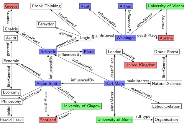
and an object o. An RDF triple can be naturally viewed as an edge with s and o as vertices. Thus, an RDF graph can be represented as a labeled directed graph, e.g., the example RDF graph G1 excerpted from DBpedia dataset in Fig. 1. It describes some information about philosophers. Due to the flexibility of RDF data, they are widely applied in various fields, such as science, bioinformatics, business intelligence,
* Yajun Yang
1 College of Intelligence and Computing, Tianjin University,
Peiyang Park Campus, Tianjin, China
2 Tianjin Key Laboratory of Cognitive Computing
and Application, Tianjin, China
3 School of Information Technology, Deakin University,
Melbourne, Australia
4 School of Information and Communication Technology,
Griffith University, Gold Coast, Australia
5 School of Information, Renmin University of China, Beijing,
and social networks [12]. In real world, the size of RDF data often reaches hundreds of millions of triples.
Subgraph matching is widely considered as one of the fundamental mechanisms for querying large-scale graph data. SPARQL is the standard query language for RDF graphs endorsed by W3C [5], in which basic graph patterns (BGP) are realization of subgraph matching. Theoretically, the semantics of SPARQL BGP is equivalent to the problem of subgraph homomorphism [18], whose evaluation com-plexity is known to be NP-complete [7]. Therefore, how to efficiently answer subgraph matching queries (i.e., BGP) over big RDF graphs has been broadly recognized as a chal-lenging problem.
Subgraph matching aims at finding all the satisfying matching subgraphs over the large data graph. More specifi-cally, given a data graph, i.e., an RDF graph G and a query graph Q, subgraph matching will fetch all the subgraphs over
G that satisfying all the triples contained in Q, which is a
conjunctivequery (CQ) on G. For instance, the following
CQQ1 consists of two triple patterns over G1.
Currently, there has been some research works on sub-graph matching queries over RDF data in a distributed
environment. One category of methods is based on the rela-tional schema [8, 11, 14, 19, 22], in which RDF data are
(1)
Q1(?x, ?y)←(𝙺𝚊𝚛𝚕_𝙼𝚊𝚛𝚡,𝚒𝚗𝚏𝚕𝚞𝚎𝚗𝚌𝚎𝙱𝚢, ?x) ∧ (𝙺𝚊𝚛𝚕_𝙼𝚊𝚛𝚡,𝚖𝚊𝚒𝚗𝙸𝚗𝚝𝚎𝚛𝚎𝚜𝚝, ?𝚢)
modeled as a set of triples and stored in relational tables or a variant relational schema. All of these methods do not consider inherent graph-like structures of RDF data. When processing complex subgraph matching queries, excessive join operations over relational tables are needed, which may incur expensive cost. In contrast, the other category of meth-ods manages RDF data in native graph formats [17, 20, 28] and represents subgraph matching queries as query graphs, which typically employs adjacency lists to store RDF data. Thus, for a subgraph matching problem, how to reduce the enormous intermediate results is crucial.
In [24], query graphs are decomposed into stars (trees of depth 1). Lai et al. pointed out that the star-join algorithm in [24] suffers from scalability problems due to the genera-tion of a large number of matches when evaluating a star with multiple edges [15]. The reason for this issue is that in unlabeled, undirected graphs, they focused on it is very likely that the large combination of intermediate results is generated due to the lack of distinguishable information on vertices and edges. Thus, they proposed the so-called
TwinTwigJoin MapReduce [6] algorithm, where a TwinTwig is either a single edge or two incident edges of a vertex. Unlike unlabeled and undirected graphs in [15, 24], RDF graphs have URIs as the unique vertex labels and directed
Greece Crook Thinking University of Vienna
Austria Chalcis Fereydon Logic Weininger Arthur Arndt Aristotle Kaut Drunk Forest Ecnomic Plato University of Bonn Natural Science Economy
Adam Smith Karl Marx
Organisation Philosophy
University of Glagow
Harold Laski Scotland
United Kingdom London Labour relation country literGenreof genreof mainInterest mainInterest country almaMater influencedBy deathPlace influencedBy deathPlace influencedBy influencedBy genreof literGenreof influencedBy mainInterest deathPlace almaMate r mainInterest fieldof countr y almaMater deathPlace mainInterest rdf:type mainInterest literGenreof country influencedBy
edges. Thus, the problem concerned in [15] does not exist over RDF graphs. Therefore, it is reasonably safe to exploit the more holistic star-shaped structures other than just twin twigs as decomposition units of query graphs to minimize the amount of intermediate results.
To this end, we propose a new star-based query decompo-sition strategy, in which the star retains more holistic graph structures of query graphs than the TwinTwig method [15]. Thus, our approach can be completed in fewer MapReduce rounds. In our method, in order to evaluate subgraph matching queries more efficiently, query graphs are decomposed into a set of stars by using the semantic and structural information embedded in RDF graph as heuristics (i.e., h values defined in this paper), to evaluate subgraph matching queries in MapRe-duce. In addition, in order to reduce the intermediate results, the matching order of stars is determined by a greedy strategy.
Our main contributions include: (1) we propose an efficient and scalable distributed algorithm based on star decomposition, called StarMR, for answering subgraph matching queries on RDF graphs; (2) two optimization strategies of StarMR are devised, one of which employ-ing the properties in RDF graphs to filter out invalid input data in MapReduce iterations, the other postponing part of Cartesian product operations to the final step of MapReduce to reduce a part of unpromising Cartesian product opera-tions; and (3) extensive experiments on both synthetic and real-world RDF graphs have been conducted to verify the efficiency and scalability of our method. On average, the experimental results show that StarMR outperforms the state-of-the-art method by an order of magnitude.
The rest of this paper is organized as follows. Section 2 briefly reviews related work. In Sect. 3, we introduce pre-liminary definitions on RDF graphs and subgraph matching queries. In Sect. 4, we describe in detail how to decom-pose CQ queries, determine the matching order of stars, and match CQ queries using MapReduce. We then present two optimization strategies in Sect. 5. Section 6 shows our extensive experimental results, and we conclude in Sect. 7.
2 Related Work
The existing research work on distributed/parallel SPARQL queries over large-scale RDF graphs can be classified as follows:
Relational Schema Approach In the context of the urgent need for Web-scale distributed query systems [29], SHARD [19] is designed and developed using the MapReduce frame-work to address the scalability limitation issue. In terms of data persistence, the metadata of the system is persisted in the Hadoop Distributed File System [23]. In that case, the query graph is decomposed into the triple sets. More specifically, SHARD handles SPARQL queries over RDF data for triple
stores which need to iterate over query statements to bind variables to vertices in data graphs while satisfying all of the query constraints. Meanwhile, to accelerate processing the subsequent similar queries, certain relevant intermediate results might not be removed immediately. Each round of MapReduce only adds one query clause with the join opera-tion in [19]. Although SHARD has a significant improve-ment in enhancing the datasets scalability with the aid of Hadoop, due to no plans for query processing, a large number of Hadoop jobs are required to execute the whole procedure.
Similarly, HadoopRDF [14] features efficiency and scal-ability in managing large amounts of RDF data. For the data stored in the Hadoop cluster, the framework utilizes a schema to convert various format RDF data to N-triples. The standard data conversion can bring great benefits for the later process-ing. Moreover, HadoopRDF divides RDF triples based on the predicates into multiple smaller files. In this way, for a user query, if the predicate position is not a variable, the corre-sponding file can be matched directly; otherwise, because the predicate is a variable, HadoopRDF cannot make sure which type of the object belongs to. To avoid searching all the files, another file organization category named object splitting is exploited. The object splitting method further classifies files according to the object type. Meanwhile, by combining the predicate and object splitting approach, the query processing can speed up. Specifically, the query retrieval involves three phases. First, regarding the subgraph matching query clause as the input and passing it to the first component named input selector. Second, making use of the proposed greedy algo-rithm to guarantee the generated query plan as the optimal one. Finally, joining the relevant intermediate items together and feeding the final results back to the user. Moreover, a triple pattern in SPARQL queries cannot simultaneously take part in more than one join in a single Hadoop job by using the MapReduce framework.
The abovementioned two methods do not employ any structural information of query graphs, thus a large number of join operations may incur expensive costs. Furthermore, Virtuoso [8], supporting RDF in a native RDBMS, also model RDF data as a set of triples. TriAD [11], using a cus-tom MPI protocol, employs six SPO permutation indexes, partitions RDF triples into those indexes, and uses a local-ity-based summary graph to speed up queries. Many cur-rent RDF query approaches are extremely dependent on the query pattern shapes, i.e., for certain query pattern shapes, the query processing can execute quite well. While the query performance drops for other query shapes. Hence, Schätzle et al. [22] proposed a relatively efficient query processing system named S2RDF, which does not depend on the query pattern shapes anymore. In addition, this approach extends the vertical partitioning [1] methods and Join Indices [25] to preprocess the original RDF data. More specifically, S2RDF introduces the relational partitioning model ExtVP to store
RDF data over the Spark parallel framework, by which it can effectively minimize the query input size. Nevertheless, as for modification operations, the deletion operation of the triples might result in a decline in query performance and stability. In addition, the cost of the semi-join preprocessing in [22] is prohibitively expensive.
Native Graph Approach The star-decomposition-based searching methods proposed by Yang et al. [26] is about approximate matching, which is devoted to top−k star query. In [26], the query decomposition phase is to decom-pose the subgraph query to a set of star queries, and for each decomposed star query, the matches in decreasing order of matching score and the best match can be picked out. In [28], RDF data are modeled in its native graph form, a key-value store which saves node identifiers as the keys, and the adja-cency lists of nodes as the values. Trinity.RDF [28] lever-ages graph exploration to reduce the volume of intermediate results, while the final results need to be enumerated at the single master node using a single thread. S2X [20] builds on GraphX [9], a distributed graph processing framework in top of Spark [27], to implement query graph matching of SPARQL. In S2X, a query graph is also decomposed into triple patterns which is similar to the methods in [14, 19]. All of these triple patterns are matched first; then, inter-mediate results are gradually discarded by iterative com-putation; finally, the remaining matching results are joined, which may lead to potentially large intermediate results. In addition, Peng et al. adopt a partial evaluation and assembly framework to perform SPARQL queries based on gStore [30], a graph-based SPARQL query engine using VS*-tree indexes [17]. In their method, each slave machine evaluates the query in the partial computation phase, and then, in the assembly phase, a large number of local partial matches are sent to the coordinator and joined together to obtain the final results, which may become a performance bottleneck when the amount of partial matches are large.
Distributed Systems In the era of Big Data, the distributed/ parallel technique has become an indispensable tool for large-scale knowledge data management. In recent years, plentiful distributed systems and frameworks for large-scale graph data have been proposed. For instance, YARS2 [13] is a representa-tive knowledge graph managing system based on MapReduce. YARS2 is a distributed semantic web search engine, which integrates data retrieving, collecting, indexing, and brows-ing together. It plays a pivotal role in managbrows-ing large-scale graph data models and enabling interactive query answering. The system consists of several components: crawler, indexer, object consolidator, index manager, query processor, ranker, and user interface. The crawler is a pipelined architecture for crawling diverse source data into a uniform schema, and the indexer is a general framework for managing keyword indices and statement indices; then, the query processor will generate the optimal query plan for answering the queries. Then, the
corresponding results are retrieved to users in the descending orders. Another research work Sempala [21], which is an RDF graph data query engine based on distributed SQL-on-Hadoop database Impala and Parquet, distributed file format, which provides interactive-time SPARQL query processing effi-ciently. In addition, Lai et al. proposed a MapReduce-based distributed efficient subgraph enumeration algorithm based on TwinTwig structure decomposition, but the algorithm is only used for undirected unlabeled graphs.
In this paper, we focus on the analytical processing scenario of RDF graphs using MapReduce which does not take advan-tage of any prebuilt indexes. Though building indexes can defi-nitely accelerate lookups with high selectivity, it will not ben-efit analytical processing in which almost all data are accessed. So, it is unfair to compare our approach with those based on intensive indexes, such as S2RDF [22], the distributed gStore system [17]. In our method, (1) we store RDF triples using the adjacency list scheme; (2) a star-decomposition strategy with heuristic information is proposed, which is able to keep more holistic structures of query graphs; (3) as to optimization strategies, we employ RDF properties to filter out unpromising input data and postpone Cartesian product operations.
3 Preliminaries
In this section, we introduce several basic background defi-nitions about RDF graphs and subgraph matching queries which are used in our algorithms.
Definition 1 (RDF graph) Let U and L be the disjoint infinite sets of URIs and literals, respectively. A tuple (s, p, o) ∈U×U× (U∪L) is called an RDF triple, where s is the subject, p is the predicate, and o is the object. A finite set of RDF triples is called an RDF graph.
Given an RDF graph G, let V, E,𝛴 denote the set of
vertices, edges, and edge labels, respectively. Formally, V = {s∣ (s, p, o) ∈G} ∪ {o∣ (s, p, o) ∈G} , E⊆V×V , and
𝛴= {p∣ (s, p, o) ∈G} . The function lab: E→𝛴 returns the
labels of edges in G.
Definition 2 (Query graph) Given an RDF graph G, a
CQ Q over G is defined as: Q(z1,…, zn)←⋀1≤i≤mtpi ,
where tpi= (xi, ai, yi) is a triple pattern, xi, yi∈
V∪Var , ai∈𝛴∪Var , zj is a variable and zj∈
{xi∣1≤i≤m} ∪ {yi∣1≤i≤m} . A CQQ is also referred
to as a query graph GQ.
Let V(Q) and E(Q) be the set of vertices and edges in GQ , respectively. For each vertex u∈V(Q) , if u∈Var , then u
can match any vertex v∈V ; otherwise, u only can match the
Definition 3 (Subgraph matching) The semantics of a CQQ
over an RDF graph G is defined as: (1) 𝜇 is a mapping from
vertices in x̄ and ȳ to vertices in V, where x̄= (x1,…, xm) ,
̄
y= (y1,…, ym) ; (2) (G,𝜇)⊨Q iff (𝜇(xi),𝜇(ai),𝜇(yi)) ∈E
and the labels of xi , ai and yi are the same as that of 𝜇(xi),𝜇(ai) and 𝜇(yi) , respectively, if xi , ai , yi ∉Var ; and (3) 𝛺(Q) is the set of 𝜇(̄z) , where (̄z) = (z1,…, zn) , such that (G,𝜇)⊨Q . 𝛺Q is the answer set of the subgraph matching query GQ over G.
Some definitions about mappings are needed. Two mappings 𝜇1 and 𝜇2 are called compatible denoted as 𝜇1∼𝜇2 , iff every element v∈dom(𝜇1) ∩dom(𝜇2) satis-fies 𝜇1(v) =𝜇2(v) , where dom(𝜇i) is the domain of 𝜇i .
Fur-thermore, the set union of two compatible mappings, i.e.,
𝜇1∪𝜇2 , is also a mapping.
4 The StarMR Algorithm
In this section, the distributed adjacency list storage strategy for an RDF graph will be first introduced. Then, we pre-sent how to decompose the query graph into a set of stars and determine the matching order of these stars. Finally, we describe in detail how to implement the subgraph matching query using MapReduce in a left-deep-join framework. 4.1 Storage Schema
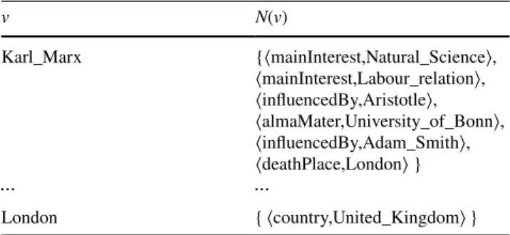
In this paper, the RDF graph G is stored in a distrib-uted adjacency list. For each vertex v∈V , we use N(v)
to denote the neighbor information of vertex v, where
N(v) = {(pi, v�i) ∣ (v, pi, v�i) ∈G} . For example, the adjacency
list storage schema of the RDF example graph G1 is given in Table 1.
Taking the RDF graph G1 in Sect. 1 as an example, all the vertices appeared in the subject positions are stored in
the first column, all the neighbor vertices of each subject vertex are stored in the set of N(v). For example, the entity
London has one outgoing edges, and its neighbor set is {⟨
country,United_Kingdom⟩}.
4.2 Star Matching
In this paper, the minimum matching unit is a star in our method, and the RDF graph G is stored in adjacency lists. Next, we give the definition of star.
Definition 4 (Star) A star is a tree of height one, denoted by T = (r, L) , where (1) r is the root of T; and (2) L is a set of 2 tuples (pi, li) , i.e., li is a leaf of T and (r, pi, li) is an edge from r to li . Let V(T) and E(T) be the set of nodes and edges in T, respectively.
When matching a star T on the adjacency list of RDF graph, if the root vertex of star T can be well matched on one of the subject vertices of the adjacency list first, the matching process will not be terminated. Then, the star T will continue matching the leaf vertices li on N(v) and once matched, we can obtain the sets of all the matching vertices, which are defined as the candidate sets S(li) in this paper. Next, we will present
the detailed process of a star matching on an adjacency list. And the star matching algorithm is listed as follows.
Table 1 The adjacency list of RDF graph G1
v N(v) Karl_Marx {⟨mainInterest,Natural_Science⟩, ⟨mainInterest,Labour_relation⟩, ⟨influencedBy,Aristotle⟩, ⟨almaMater,University_of_Bonn⟩, ⟨influencedBy,Adam_Smith⟩, ⟨deathPlace,London⟩ } ⋯ ⋯ London {⟨country,United_Kingdom⟩} Algorithm 1: StarMatch(T, N(v))
Input : Star:T = (r, L), whereL={(p1, l1), . . . ,(pt, lt)},N(v), v∈V
Output: Matching results ofT overN(v):Ωv(T) ={µ1, µ2, ..., µn} 1 Ωv(T)← ∅;
2 if T.rmatches vertexvthen
3 foreach(pi, li)∈T.Ldo // the candidate set S(li) of leaf li 4 if pi∈/V arthen
5 S(li)← {v|(pi, v)∈N(v)∧limatchesv};
6 else // is a wildcard
7 S(li)← {v|( , v)∈N(v)∧limatchesv};
// do Cartesian product operation {v} ×S(l1). . . S(lt) to get Ωv(T) 8 Ωv(T)← {µ∪µ1. . . µt|µ={(T.r, v)} ∧µi={(li, v)}, li∈T.L∧v∈S(li)}; 9 returnΩv(T);
Algorithm 1 will be run in the following steps: (1) first matches the root T.r with the vertex v (line 2); (2) then obtains the candidate matching set of every leaf (lines 3–7); (3) next does the Cartesian product operations on the can-didate matching sets of vertices in the star T to get match-ing results (line 8). Finally, StarMatch(T, N(v)) returns the matching results of the star T over N(v) (line 9), and 𝛺(T) is
the union of 𝛺v(T) , where v∈V.
4.3 Star Decomposition of Query Graphs
Before matching the subgraphs in an RDF graph, it is neces-sary to decompose the query graph into the minimum match-ing unit stars. Next, we give the definition of star decom-position and explain why the matching orders are crucial.
In addition, we propose an effective approach to reduce the number of intermediate results, which leverages the user-defined heuristic information h value.
Definition 5 (Star decomposition) The star decomposition
of a CQQ= {tp1,…, tpn} is denoted as D= {T1,…, Tm} , where (1) Ti is a star; (2) Ti.r≠Tj.r, Ti, Tj∈D∧i≠j ; ( 3 ) E(Ti) ∩E(Tj) = �, Ti, Tj∈D∧i≠j ; a n d ( 4 ) ⋃
1≤i≤mE(Ti) =E(Q).
Example 1 Consider the example query Q1 over the RDF graph G1 in Sect. 1, the query graph GQ1 of Q1 is shown in
Fig. 2. Moreover, D is the star decomposition of GQ
1 which
contains three stars, T1 , T2 , and T3 . □ GQ1 ?h ?k ?x ?y ?w ?z ?d ?g influencedBy influencedBy mainInterest literaryGenreof genreof almaMater deathPlace country D ?y ?w ?g genreof litera ryGenreof T1 (T2) ?x ?h ?k ?y ?d ?z influencedBy influencedBy mainInterest deathPlace almaMater T2 (T1) ?z country ?d T3 (T3) P ?x ?h ?k ?y ?d ?z influencedBy influencedBy mainInterest deathPlace almaMater P1 ?h ?k ?x ?y ?w ?z ?d ?g influencedBy influencedBy mainInterest litera ryGenreof genreof almaMater deathPlace P2 ?h ?k ?x ?y ?w ?z ?d ?g influencedBy influencedBy mainInterest litera ryGenreof genreof almaMater deathPlace country P3
After obtaining the query decomposition D of Q1 , there exist six matching orders. According to Algorithm 1, stars
T1, T2 , and T3 over G1 have 2, 2, and 4 matching results,
respectively. Consider the matching order T1T3T2 , there
exists eight intermediate results by joining the matching results of star T1 and T3 , because these two stars do not share
any common vertex. However, another matching order
T2T1T3 only generates one intermediate result. In other
words, the matching order of stars has a significant effect on the performance of queries.
We leverage the structure information and semantics in RDF graphs to decompose the query graph into stars and give a matching order to reduce the number of inter-mediate results using a greedy strategy. In particular, we define h value as the heuristic information. The func-tion fre: 𝛴→ℕ gets the frequency of a predicate p in an
RDF graph G, where ℕ is the set of natural numbers and fre(p) =|{(si, p, oi) ∣ (si, p, oi) ∈G}| . Then, for a query Q
over G, let P(u) be the set of properties (a.k.a., predicates) of vertex u in Q, i.e., P(u) = {pi∣ (u, pi, u�i) ∈Q} . The h value
of each vertex u∈V(Q) is defined as follows:
where outDeg is the out degree of vertex u. The h value is determined by two factors: (1) the more out degrees a vertex u has, the more variables may be bound when the star rooted at u is matched; (2) the smaller 𝖿 𝗋𝖾(p), p∈P(u) is, the
higher selectivity of vertex u has. If all properties of vertex
u are variables, h(u) =0 . Our star-decomposition algorithm guided by h values is shown in Algorithm 2.
(2) 𝗁(u) = |outDeg|
minp∈P(u)𝖿 𝗋𝖾(p)
In Algorithm 2, a constant vertex in Qc having the
maxi-mum h value is selected as the root of the first star (lines 3–4). If Qc is an empty set, the algorithm picks up a vertex
in Sub(Q) whose h value is the maximum (lines 4–5). The star rooted at the selected vertex is generated (line 7) by call-ing the function genStar (lines 13–17). Then, we use Mv to
denote the candidate set of root nodes which can guarantee that the star to be generated and the stars that have been gen-erated share at least one common vertex (line 9). Similarly, after obtaining the vertex r with respect to the h value, a new star is generated (lines 10–11). This process (lines 8–11) terminates until the set Q is empty.
For a subgraph matching query Q, Algorithm 2 can pro-duce a star decomposition D and determine an order of these stars, T1…Tm , such that
⋃
1≤i<jV(Ti)∩V(Tj)≠� , 1≤j≤m .
Based on this matching order, we further introduce the con-cept of the partial query graph.
Definition 6 (Partial query graph) The partial query graph Pj, 1≤j≤m is a subgraph of GQ , where (1) V(Pj) =⋃1≤i≤jV(Ti) and (2) E(Pj) =
⋃
1≤i≤jE(Ti) .
Obviously, P1=T1 and Pm=GQ . Let 𝛺(Ti) and 𝛺(Pi)
be the set of matching results for star Ti and partial
query graph Pi , respectively. We have 𝛺(P1) =𝛺(T1) ,
𝛺(Pt) =𝛺(Pt−1)⋈𝛺(Tt) , and 𝛺(Pm) =𝛺(Q).
Example 2 Consider the query Q1 over G1 , where h(?y) = 2
3 , h(?x) = 4
2 , and h(?z) = 1
4 . According to Algorithm 2, the first
selected vertex is ?x and the corresponding star is T2 ( T1 ) in ′
Fig. 2. Then, stars T1 ( T2′ ) and T3 ( T3′ ) are generated. Based
on this order, P1, P2 , and P3 in Fig. 2 are the partial query
Algorithm 2: StarDecompose(Q)
Input : A Query graphQ:{tp1, tp2, ..., tpn}
Output: A Queue of starsD:{T1, ..., Tm}
1 D← ∅; // D: the queue of stars, V(D): the set of vertices in D 2 Qc← {s|s∈Sub(Q)∧s /∈V ar}; // Sub(Q): the set of subjects in Q 3 if Qc=∅then
4 r←arg maxv∈Qch(v)
5 else
6 r←arg maxv∈Sub(Q)h(v)
7 genStar(r, Q, D); // generate the star rooted at vertex r
8 whileQ=∅do
9 Mv← {s|s∈Sub(Q)∧s∈V(D)} ∪ {s|(s, p, o)∈Q∧o∈V(D)}; 10 r←arg maxv∈Mvh(v);
11 genStar(r, Q, D);
12 returnD:{T1, ..., Tm};
13 FunctiongenStar(r, Q, D) // generate a star
14 T.r←r;
15 T.L← {(pi, li)|(r, pi, li)∈Q}; 16 D.enqueue(T);
graphs of Q1 . Obviously, P3 is exactly the original query graph GQ
1 . □
4.4 Subgraph Matching Algorithm Using MapReduce
Next, we show how to use MapReduce to answer a subgraph matching query in a left-deep-join framework and demon-strate the pseudocode of our StarMR algorithm.
We can get P1=T1 and Pm=GQ according to the partial
query graph definition. In addition, the notation 𝛺(Ti) repre-sents the matching results of the star Ti . The notation 𝛺(Pi)
represents the matching results of the partial query graph
Pi . The partial query graph Pi can be obtained by joining
the star Ti and partial query graph Pi−1 together. Thus, the
intersection of Pi−1 and Ti will serve as the joining key. To process the subgraph matching query efficiently, we present Algorithm 3 to answer the queries, which uses MapReduce.
Algorithm 3 decomposes the query Q into a queue K of stars (line 1) and matches these stars in MapReduce itera-tions (lines 3–9). Each round of the MapReduce iteration joins one star with the partial results until all stars are matched. Map function consists of two parts: (1) when the input value is N(v) (lines 12–20), the function matches the star Tt over every neighbor information N(v) in RDF graph
Gin parallel (line 13), then let the matching results of inter-section of vertex sets of star Tt and partial query graph Pt−1 , i.e., 𝜇key , be keys (line 22); and (2) when the input value is
a mapping in 𝛺(Pt−1) (lines 22–23), similarly, let 𝜇key be
keys (line 20). Every mapping 𝜇 in 𝛺v(Tt) and 𝛺(Pt−1) is transformed into a key-value pair (𝜇key,𝜇) . Note that when
t=1 , the output of map is (�,𝜇) (lines 14–16). reduce
func-tion joins the matching results of Tt and Pt−1 to generate the
matching results of Pt with 𝜇key as the keys (lines 24–26).
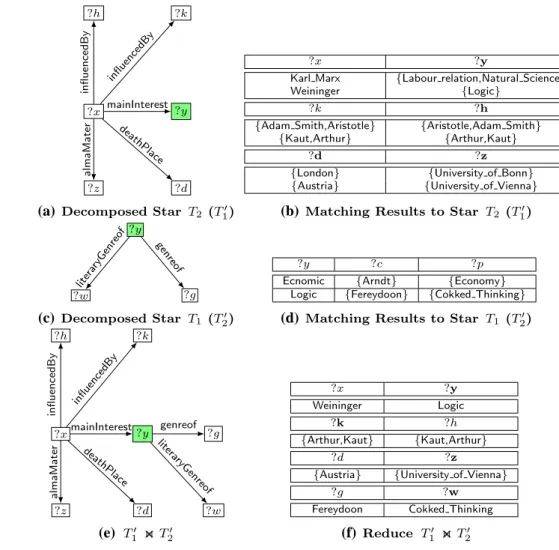
Figure 3 shows the matching process of StarMR.
Theorem 1 Given an RDF graphGand a query graphGQ ,
we assume that Algorithm 2 decomposesGQinto a queue of
Algorithm 3: StarMR
Input : RDF graphG= (V, E, Σ), A query graphQ:{tp1, tp2, ..., tpn}
Output: The answer set:Ω(Q)
1 K ←StarDecompose(Q); // decompose query graph
2 Ω(Q)← ∅,t←1;
3 whileK is not emptydo // MapReduce iterations
4 Tt←K.dequeue(); 5 map(∅, N(v)); 6 if t >1then 7 map(∅, µ) s.t.µ∈Ω(Pt−1); 8 reduce(µkey,(Ω1, Ω2) s.t.Ω1⊆Ω(Tt)∧Ω2⊆Ω(Pt−1)); 9 t←t+ 1; 10 returnΩ(Pm); 11 Functionmap(∅,N(v)orµ)
12 if value is an adjacency listN(v)inGthen // match the star Tt 13 Ωv(Tt)←starM atch(Tt, N(v)) ;
14 if t= 1then
15 foreachµ∈Ωv(T1)do 16 return(∅, µ) ;
17 else
18 foreachµ∈Ωv(Tt)do // get the mapping µkey as key 19 µkey← {(uk, µ(uk))|uk∈V(Pt−1)∩V(Tt)};
20 return(µkey, µ);
21 else // value is a mapping
22 µkey← {(uk, µ(uk))|uk∈V(Pt−1)∩V(Tt)}; 23 return(µkey, µ) ;
24 Functionreduce(µkey,(Ω1, Ω2))
25 foreach(µ, µ)∈Ω1×Ω2do
starsD= {T1,…, Tm} . Algorithm 3 gives the correct query
results, and the number of MapReduce iterations ism.
Proof (Sketch) The algorithm correctness can be proved as follows: (i) In the first MapReduce iteration of Algorithm 3, Algorithm 1 is invoked by the map function to match the star T1 ; then, the matching set 𝛺(T1) , i.e., 𝛺(P1), can be obtained. From the second round of the MapReduce iteration on, Algo-rithm 3 matches a new star Tt in each round according to the
matching orders computed by Algorithm 2. In this way, the star matching result 𝛺(Tt) can be given out. (ii) In the reduce function, the matching results 𝛺(Pt−1) and 𝛺(Tt) are joined, and the joining results 𝛺(Pt) can be obtained, where 𝛺(Pt−1) is the matching results of partial query graph Pt−1 , which is obtained in the last round of the MapReduce iteration. Con-sequently, the answer set of query Q, i.e., 𝛺(Pm), can be
obtained in the m round of the MapReduce iteration. □ Theorem 2 The time complexity of Algorithm 3 is bounded byO(|V|m
⋅|Nmax|m⋅|Lmax|) , where |V| is the size ofG, |Nmax|
Fig. 3 Matching stars with the
basic algorithm 𝐒𝐭𝐚𝐫𝐌𝐑 ?x ?h ?k ?y ?d ?z influencedBy influencedBy mainInterest deathPlace almaMater
(a) Decomposed Star T2 (T1)
?x ?y ?k
Karl Marx Labour relation Adam Smith Karl Marx Labour relation Aristotle
Karl Marx Natural Science Adam Smith Karl Marx Natural Science Aristotle Weininger Logic Kaut Weininger Logic Arthur
?h ?d ?z
Aristotle London University of Bonn Adam Smith London University of Bonn Aristotle London University of Bonn
Adam Smith London University of Bonn Arthur Austria University of Vienna
Kaut Austria University of Vienna
(b) Matching T2 (T1) with StarMR
?y ?w ?g genreof litera ryGenreof (c)Decomposed Star T1 (T2) ?y ?c ?p
Ecnomic Arndt Economy Logic Fereydoon Cokked Thinking
(d) Matching T1 (T2) with StarMR
?h ?k ?x ?y ?w ?z ?d ?g influencedBy influencedBy mainInterest litera ryGenreof genreof almaMater deathPlace (e) T1 T2 ?x ?y Weininger Logic Weininger Logic ?k ?h Arthur Kaut Kaut Arthur ?d ?z
Austria University of Vienna Austria University of Vienna
?g ?w
Arndt Economy Fereydoon Cokked Thinking
(f) Reduce T1 T2
is the largest out degree inG, and |Lmax|is the largest out
degree inGQ.
Proof (Sketch) In Algorithm 3, each round of the MapRe-duce iteration matches one star; therefore, it can evaluate the query Q in m rounds. The time complexity of Algorithm 3 consists of two parts: (1) the time complexity of star match-ing is ∑1≤t≤m
∑
v∈V(�N(v)�+�𝛺(Tt)�) ; (2) the time complex-ity of join operations is ∑1<t≤m�𝛺(Pt−1)�×�𝛺(Tt)� . In the worst case, every leaf in Tt can match all neighboring ver-tices of a vertex v, v∈V , i.e., |𝛺v(Tt)|=|N(v)||Tt.L| . Thus, the time complexity of Algorithm 3 is bounded by O(|V|m
⋅
|Nmax|m⋅|Lmax|)
□
5 Two Optimization Strategies
In this section, two optimization strategies are proposed to improve the efficiency of the StarMR algorithm. The first one
leverages the inherent semantics of the RDF graph to reduce the overhead expense; the other technique improves the query performance by postponing the Cartesian product operations.
5.1 RDF Property Filtering
We take advantage of the inherent semantics embedded in RDF graphs to filter out unpromising computations. As mentioned in Sect. 1, the RDF describes resources by defin-ing classes and properties. In addition, the RDF Schema (RDFS)2 is an extended version of RDF, which is regarded as a framework to define classes of resources. For instance, the RDF triple (s,𝚛𝚍𝚏∶𝚝𝚢𝚙𝚎, C) declares that resource s is an instance of the class C, denoted by s∈C . We assume that
for each subject s in an RDF graph G, there exists at least a triple (s,𝚛𝚍𝚏∶𝚝𝚢𝚙𝚎, C) ∈G . We believe that this
assump-tion is reasonable since every resource should belong to at least one type in the real world.
Example 3 As shown in Fig. 1, the triple
(𝚄𝚗𝚒𝚟𝚎𝚛𝚜𝚒𝚝𝚢_𝚘𝚏_𝙱𝚘𝚗𝚗, 𝚛𝚍𝚏∶𝚝𝚢𝚙𝚎, 𝙾𝚛𝚐𝚊𝚗𝚒𝚜𝚊𝚝𝚒𝚘𝚗)
denotes that University_of_Bonn is an instance of
the class Organization. Other such triples in Fig. 1 are
omitted. Moreover, all instances of class 𝙾𝚛𝚐𝚊𝚗𝚒𝚜𝚊𝚝𝚒𝚘𝚗 are
highlighted in green. Similarly, there exist other classes in G1 , e.g., Person in blue and Country in red. □
G i ve n a n R D F g r a p h G= (V, E,𝛴) , l et
P�(C) = {p∣ (s, p, o) ∈G∧s∈C} be the set of RDF prop-erties of class C. Note that the size of classes in an RDF graph is much less than vertices in the corresponding RDF graph. When matching a star T in the function Map(T, N(v)), RDF properties of C can be used to filter out input data as follows: if v∈C∧P(T.r)⊈P�(C) , the procedure starMatch(T, N(v)) in map function can be pruned.
Example 4 Consider matching star T2 rooted at ?x in Fig. 2 over G1
in Fig. 1, we have P(?x) = {𝚒𝚗𝚏𝚕𝚞𝚎𝚗𝚌𝚎𝚍𝙱𝚢,𝚖𝚊𝚒𝚗𝙸𝚗𝚝𝚎𝚛𝚎𝚜𝚝,
𝚍𝚎𝚊𝚝𝚑𝙿𝚕𝚊𝚌𝚎,𝚊𝚕𝚖𝚊𝙼𝚊𝚝𝚎𝚛} a n d P�(𝙾𝚛𝚐𝚊𝚗𝚒𝚜𝚊𝚝𝚒𝚘𝚗) =
{𝚌𝚘𝚞𝚗𝚝𝚛𝚢} . Due to 𝚄𝚗𝚒𝚟𝚎𝚛𝚜𝚒𝚝𝚢_𝚘𝚏_𝙶𝚕𝚊𝚐𝚘𝚠∈𝙾𝚛𝚐𝚊−
𝚗𝚒𝚜𝚊𝚝𝚒𝚘𝚗∧P(?x)⊈P�(𝙾𝚛𝚐𝚊𝚗𝚒𝚜𝚊𝚝𝚒𝚘𝚗) , the computation of starMatch(T2 , N(𝚄𝚗𝚒𝚟𝚎𝚛𝚜𝚒𝚝𝚢_𝚘𝚏_𝙶𝚕𝚊𝚐𝚘𝚠)) can be
pruned. □
5.2 Postponing Cartesian Product Operations In this section, we first demonstrate the expensive cost introduced by our basic algorithm and then illustrate an
Fig. 4 Matching stars with the optimization algorithm
𝐒𝐭𝐚𝐫𝐌𝐑𝐨𝐩𝐭 ?x ?h ?k ?y ?d ?z influencedBy influencedBy mainInterest deathPlace almaMater
(a) Decomposed Star T2 (T
1)
?x ?y
Karl Marx {Labour relation,Natural Science} Weininger {Logic}
?k ?h
{Adam Smith,Aristotle} {Aristotle,Adam Smith} {Kaut,Arthur} {Arthur,Kaut}
?d ?z
{London} {University of Bonn} {Austria} {University of Vienna}
(b) Matching Results to Star T2 (T
1) ?y ?w ?g genreof litera ryGenreof (c)Decomposed Star T1 (T 2) ?y ?c ?p
Ecnomic {Arndt} {Economy} Logic {Fereydoon} {Cokked Thinking}
(d) Matching Results to Star T1 (T
2) ?h ?k ?x ?y ?w ?z ?d ?g influencedBy influencedBy mainInterest litera ryGenreof genreof almaMater deathPlace (e) T 1 T2 ?x ?y Weininger Logic ?k ?h {Arthur,Kaut} {Kaut,Arthur} ?d ?z
{Austria} {University of Vienna}
?g ?w
Fereydoon Cokked Thinking
(f) Reduce T
1 T2
efficient solution. Finally, the optimization method will be analyzed.
In the initial star matching phase of our basic algorithm
StarMR, the function map is invoked to match the star T1 ,
where T1= (r, L) and L= {(p1, l1),…,(pt, lt)} ; then, we can
obtain the candidate matching set S(li) of every leaf vertex
li . The matching set S(li) is generated according to the label
of li matched with leaf vertices over N(v). Next, we can get
the matching results by doing the Cartesian product opera-tions on the candidate matching sets of vertices in the star T1 .
Unfortunately, a majority of matching results cannot contrib-ute to the final results. In other words, the Cartesian product operation is not necessarily done during the star matching
phase. Even worse, that operation can incur expensive cost in addition. Since the Cartesian product operation leads to expensive costs, after executing subgraph matching with our basic algorithm StarMR, an improvement is proposed to postpone the Cartesian product operation.
Let f be a mapping from vertices in a star to the candidate matching sets of the corresponding vertices. We use 𝛺�(T)
and 𝛺�(P) to denote the matching results of star T and partial
query graph P, respectively. In order to reduce the intermedi-ate results cost. We develop an efficient optimization algo-rithm, denoted by StarMRopt . In our optimization method,
the initial star matching phase only needs to calculate the candidate matching sets of leaves of the star T1.
Algorithm 4: StarMRopt
Input : RDF graphG= (V, E, Σ), A subgraph matchingQ:{tp1, tp2, ..., tpn}
Output: The answer set:Ω(Q)
1 K ←StarDecompose(Q); // decompose query graph
2 Ω(Q)← ∅,t←1;
3 whileK is not emptydo // MapReduce iterations
4 Tt←K.dequeue(); 5 map(∅, N(v)); 6 if t >1then 7 map(∅, µ) s.t.µ∈Ω(Pt−1); 8 reduce(µkey,(Ω1, Ω2) s.t.Ω1⊆Ω(Tt)∧Ω2⊆Ω(Pt−1)); 9 t←t+ 1; 10 returnΩ(Pm);
11 FunctionstarM atchopt(T, N(v)) // Cartesian product can be postponed. 12 if T.rmatches vertexvthen
13 foreach(pi, li)∈T.Ldo 14 if pi∈/V arthen 15 S(li)← {v|(pi, v)∈N(v)∧li matchesv}; 16 else 17 S(li)← {v|(, v)∈N(v)∧li matchesv}; 18 f← {(u, S(u))|u∈V(T)}; 19 returnf;
20 Functionmap(∅,N(v)orfs.t.t >1) // RDF property filtering is applied.
21 if t= 1then
22 return(∅, starM atchopt(T1, N(v)));
23 else
24 Vkey:{u1, . . . , uk} ←V(Pt−1)∩V(Tt); 25 if value is an adjacency listN(v)inGthen 26 f←starM atchopt(Tt, N(v));
// do f(u1)× · · · ×f(uk) to get Ωkey
27 Ωkey← {f1∪ · · · ∪fk|fi={(ui,{v})} ∧ui∈Vkey∧v∈f(ui)};
28 foreachfkey ∈Ωkey do // f∈Ωf
29 return(fkey, f−Vkey);
30 else
31 Ωkey← {f1∪ · · · ∪fk |fi={(ui,{v})} ∧ui∈Vkey∧v∈f(ui)};
32 foreachfkey ∈Ωkey do // f∈Ωf
33 return(fkey, f−Vkey); 34 Functionreduce(fkey,(Ωf, Ωf))
35 foreach(f, f)∈Ωf×Ωf do
I n A l g o r i t h m 1 , f o r e a c h s t a r
T= (r, L), L= {(p1, l1),…,(pt, lt)} , we do the Cartesian product operation {v} ×S(l1) …S(lt) to get the matching
results of the star T over N(v), which is 𝛺v(T) . However,
unlike Algorithm 1 enumerating the matching results of each leaf node in detail, the starMatchopt(T, N(v)) method
adds (u, S(u)) to a mapping f (line 18). Similarly, the func-tions map and reduce are also changed. In the first itera-tion, the function map invokes the starMatchopt(T, N(v)) method and return the mapping f. Meanwhile, in the t-th MapReduce iteration, first joining the t-th star Tt with the
partial query graph Pt−1 ; then, the common vertices key
sets Vkey∶ {u1,…, uk} can be obtained. (line 19). The input of the function map can be classified into two categories.
One is an adjacency list N(v) in G; the other is a mapping
f. The map function does the Cartesian product operation f(u1) ×⋯×f(uk) , where uk∈V(Pt−1) ∩V(Tt) (lines 22–33).
The reduce function takes (k, v) pairs as the input, and for those (k, v) pairs with the same key, the reduce function can
join them together and emerge a new (k, v) pair. For every f ∈𝛺�(P
m) , we do the remaining Cartesian product
opera-tion f(u�1) ×⋯×f(u�k) to get the final matching results 𝛺(Q) ,
where u�k∈V(Q)⧵⋃1<t≤m(Pt−1∩V(Tt)) (lines 19–20). Although the strategy does not change the complexity of our algorithm, they can improve query efficiency significantly. We will take an example to further illustrate the optimiza-tion algorithm.
Example 5 When answering Q1 over G1 ,
star-Match(T1�, N(𝙺𝚊𝚛𝚕_𝙼𝚊𝚛𝚡)) obtains the candidate setS(li)
of every leaf li in T1 , e.g., ′ S(?y) = {𝙽𝚊𝚝𝚞𝚛𝚊𝚕_𝚂𝚌𝚒−𝚎𝚗𝚌𝚎} .
We have V(P1) ∩V(T2�) = {?y} . Next, star T
′
2 is matched, but
the candidate set of ?y in all N(v) in G1 does not contain vertex Natural_Science. Thus, we do not need to do
the Cartesian product operation S(?z) ×S(?y) ×S(?w) to get
𝛺𝙺𝚊𝚛𝚕_𝙼𝚊𝚛𝚡(T1�) , whose cost is prohibitively expensive. The
more detailed explanation could refer to Figs. 3 and 4.
□
6 Experiments
We have carried out extensive experiments on both synthetic and real-world RDF graphs to verify the efficiency and scal-ability of StarMR and compared it with the optimization method StarMRopt , the state-of-the-art S2X, and SHARD.
Our algorithm is orthogonal to the graph partitioning and placement strategies in the cluster environment. In particu-lar, for the implementation of StarMR, we use the default partitioner employed by the Hadoop Distributed File System (HDFS).
6.1 Settings
The prototype program, which is implemented in Scala using Spark, is deployed on an 8-site cluster connected by a gigabit Ethernet. Each site has a Intel(R) Core(TM) i7-7700 CPU with four cores of 3.60GHz, 16GB memory, and 500GB disk. We used Hadoop 2.7.4 and Spark 2.2.0. All the experiments are carried out on Linux (64-bit CentOS) operating systems.
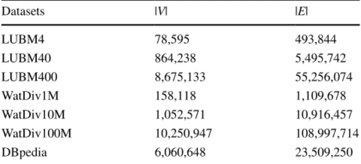
We used three RDF datasets, including synthetic data-set WatDiv,3 LUBM,4 and real-world dataset DBpedia5 in our experiments. (1) WatDiv is an RDF benchmark, which allows users to define their own datasets and generate test datasets with different sizes; (2)LUBM is also a standard RDF synthetic benchmark, which is used to generate data-sets of different scales; (3) DBpedia is a real-world dataset extracted from Wikipedia. As listed in Table 2, we sum-marize the statistics of these datasets. For RDF queries, we group them into four categories according to their shapes, including linear queries (L), star queries (S), snowflake
queries (F), and complex queries (C), which are listed in Table 3. Regarding WatDiv, it gives 20 basic query tem-plates. We leveraged 14 testing queries provided by the LUBM benchmark. Due to the absence of query templates on DBpedia, we designed eight queries, covering the four query categories mentioned above.
6.2 Experiments on WatDiv Datasets
In this section, we verify the efficiency and scalability of our methods on WatDiv datasets. This section is organized as the following orders: (1) brief introduction on WatDiv data-set; (2) validate the efficiency of the optimization algorithm
StarMRopt and analyze the experimental results; (3) examine the scalability of these methods.
Waterloo SPARQL Diversity Test Suite [2], denoted by WatDiv, was developed to measure the performance of an RDF data management system, i.e., the RDF data scale and the SPARQL queries spectrum can be defined by the user themselves. More specifically, WatDiv is composed of a data generator and a query generator. We can generate our own datasets through a designated dataset description language using the data generator. Our experiments were carried out on WatDiv1M, WatDiv10M, and WatDiv100M datasets, where “1M” indicates the number of triples is one million.
3 http://dsg.uwate rloo.ca/watdi v/. 4 http://swat.cse.lehig h.edu/proje cts/lubm/. 5 http://wiki.dbped ia.org/downl oads-2016-10.
6.2.1 Efficiency on WatDiv
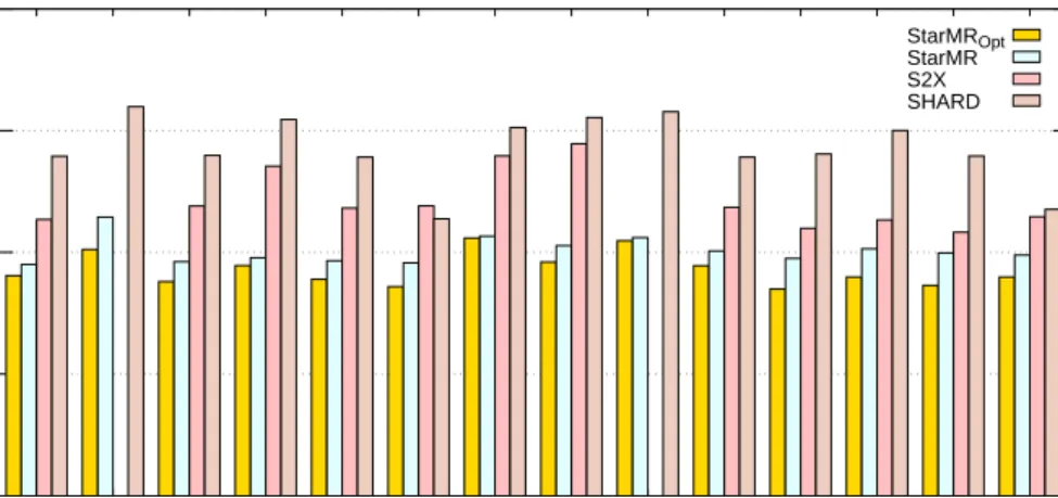
Experiments were conducted on WatDiv100M to verify the query efficiency of our method. As shown in Fig. 5, our optimization method StarMRopt has the best query efficiency
on all 20 queries. The basic method StarMR is also much
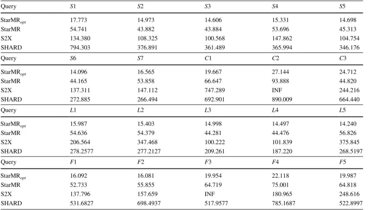
better than S2X and SHARD. The query execution times of these 20 queries are given in Table 4. For the query F3
(resp. C2 ), it can be observed that S2X cannot finish in the
time limit ( 1×10⁴s ), denoted by INF, while StarMR opt and
StarMR can return the answers within 20s (resp. 28s) and 65s (resp. 94s), respectively. The average execution speed
of the remaining 18 queries in StarMRopt is about 11 times
faster than of that in S2X. Furthermore, the average query execution time of StarMRopt covering all the query catego-ries is about 17 seconds, which is up to 47 times and on average 26 times faster than SHARD, i.e., our optimization method on average, outperforms S2X and SHARD by an order of magnitude over WatDiv100M.
In addition, compared with StarMR, the time of
StarMRopt is reduced from 44.86% to 74.94%, as listed in
Table 4. Thus, StarMRopt is able to evaluate the query more
efficiently. We can observe that StarMRopt tends to be stable over all the queries. In contrast, S2X and SHARD fluctuate dramatically.
The experimental result demonstrates that the effect of optimization strategies in StarMRopt is significant. We ana-lyze that the reasons include: (1) S2X and SHARD joined the intermediate matching results of all triple patterns in subgraph and did not leverage any structure and semantic information, leading to expensive cost; (2) StarMR did
Car-tesian product operations in the star matching phase, which may lead to expensive cost; and (3) in StarMRopt , a part of
invalid input data were pruned by utilizing RDF properties embedded in RDF graphs, and a large number of Cartesian operations were postponed and reduced.
6.2.2 Scalability on WatDiv
We compared StarMRopt with StarMR, S2X, and SHARD. The scalability comparison experiments were carried out on various scale WatDiv datasets and different experimental cluster sites.
Different Size of Datasets For the reason that S2X cannot finish in the time limit ( 1×10⁴s ) on query F
3 and C2 , we
conducted experiments on WatDiv datasets over the other 18 queries except them. Moreover, the average times of
Table 2 Datasets Datasets |V| |E| LUBM4 78,595 493,844 LUBM40 864,238 5,495,742 LUBM400 8,675,133 55,256,074 WatDiv1M 158,118 1,109,678 WatDiv10M 1,052,571 10,916,457 WatDiv100M 10,250,947 108,997,714 DBpedia 6,060,648 23,509,250 Table 3 Queries Query L S F C LUBM Q1, Q3, Q5, Q6, Q10, Q11, Q13, Q14 Q4 Q7, Q8, Q12 Q2, Q9 WatDiv L1, L2, L3, L4, L5 S1, S2, S3, S4, S5, S6, S7 F1, F2, F3, F4, F5 C1, C2, C3 DBpedia L1, L2 S1, S2 F1, F2 C1, C2
Fig. 5 The results on different queries over WatDiv100M
100 101 102 103 INF L1 L2 L3 L4 L5 S1 S2 S3 S4 S5 S6 S7 F1 F2 F3 F4 F5 C1 C2 C3 Query Time (s) WatDiv100M StarMRopt StarMR S2X SHARD
Table 4 The query times (in s) of StarMRopt , StarMR, S2X, and SHARD on WatDiv100M Query S1 S2 S3 S4 S5 StarMRopt 17.773 14.973 14.606 15.331 14.698 StarMR 54.741 43.882 43.884 53.696 45.313 S2X 134.380 108.325 100.568 147.862 104.754 SHARD 794.303 376.891 361.489 365.994 346.176 Query S6 S7 C1 C2 C3 StarMRopt 14.096 16.565 19.667 27.144 24.712 StarMR 44.165 53.858 66.647 93.888 44.820 S2X 137.311 147.112 747.289 INF 244.216 SHARD 272.885 266.494 692.901 890.009 664.440 Query L1 L2 L3 L4 L5 StarMRopt 15.987 15.403 14.998 14.497 14.240 StarMR 54.636 54.379 44.281 44.476 56.826 S2X 206.564 347.468 100.222 101.839 375.845 SHARD 278.2577 277.2127 209.261 187.220 268.5197 Query F1 F2 F3 F4 F5 StarMRopt 16.092 16.081 19.954 22.118 19.987 StarMR 52.733 55.855 64.719 75.001 64.818 S2X 137.796 157.659 INF 180.965 248.616 SHARD 531.6827 698.4937 517.9577 785.1687 522.8997
Fig. 6 Scalability on WatDiv datasets 0 52 104 156 208 260 1M 10M 100M Query Time (s) (a) Linear StarMRopt StarMR S2X SHARD 0 84 168 252 336 420 1M 10M 100M Query Time (s) (b) Star StarMRopt StarMR S2X SHARD 0 130 260 390 520 650 1M 10M 100M Query Time (s) (c) Snowflake StarMRopt StarMR S2X SHARD 0 164 328 492 656 820 1M 10M 100M Query Time (s) (d) Complex StarMRopt StarMR S2X SHARD
each query category were calculated, as shown in Fig. 6. When changing the size of datasets from WatDiv1M to Wat-Div100M, query times of all four methods increased and
StarMRopt was always the best one. We can observe that
with the scale of the datasets increasing, the query times of S2X and SHARD increased dramatically. More specifically, the average growth rate of S2X and SHARD were 95.8% and 72.7%, respectively. In contrast, for the two methods
StarMRopt and StarMR, the query time growth rate changed
slightly. We analyzed the low performance of S2X and
SHARD was that the expensive cost incurred by abundant intermediate results.
Compared with StarMRopt , the growth rate of query times in StarMR was higher than that of StarMRopt . As
shown in Fig. 6, the performance of SHARD and S2X dropped significantly with the size of datasets increasing, especially SHARD.
Different Numbers of Cluster Sites Extensive experiments were carried out on the WatDiv100M dataset with the num-ber of cluster sites varying from 4 to 8. During these experi-ments, we randomly selected one query from each of the four
Fig. 7 Scalability on cluster sites 0 140 280 420 560 700 4 5 6 7 8 Query Time (s)
(a) Query L4 over WatDiv100M StarMRopt StarMR S2X SHARD 100 101 102 103 104 105 4 5 6 7 8 Query Time (s)
(b) Query S4 over WatDiv100M StarMRopt StarMR S2X SHARD 100 101 102 103 104 105 4 5 6 7 8 Query Time (s)
(c) Query F2 over WatDiv100M StarMRopt StarMR S2X SHARD 100 101 102 103 104 105 4 5 6 7 8 Query Time (s)
(d) Query C3 over WatDiv100M StarMRopt
StarMR S2X SHARD
Fig. 8 Efficiency on LUBM40
10-1 100 101 102 103 Q1 Q2 Q3 Q4 Q5 Q6 Q7 Q8 Q9 Q10 Q11 Q12 Q13 Q14 Query Time(s) LUBM40 StarMROpt StarMR S2X SHARD
query categories, i.e., L4, S4, F2 , and C3 . As shown in Fig. 7,
the experimental results verified our intuition that query times of all these four methods decreased as the number of cluster sites increased. This is because when the number of sites increased, the degree of parallelism also increased. Although with the number of sites increasing, the speedup ratios of S2X and StarMRopt are comparative; the perfor-mance of StarMRopt is stable for selective queries and the query times of StarMRopt are far less than that of S2X. For
SHARD, we can observe that the query times of category F
and S are around 1000 s, and in all the query categories, the query time of SHARD dropped dramatically from site 4 to site 5. It demonstrated that the performance of SHARD was extremely dependent on the experimental environment. 6.3 Experiments on LUBM
The Lehigh University Benchmark [10], denoted by LUBM, is a synthetic dataset, which aims at evaluating the perfor-mance and capability of various knowledge base systems. To verify the stability of StarMRopt , extensive experiments
were conducted not only on the WatDiv datasets but also on the standard benchmark LUBM. In this paper, we use the LUBM datasets scaling from LUBM4 to LUBM400. The
following experiments focus on two aspects: the efficiency and scalability of these methods.
6.3.1 Efficiency on LUBM
The efficiency validating experiments were conducted on the LUBM40 dataset. Figure 8 compared our proposed methods
StarMRopt and StarMR with the other two methods.
We can observe that StarMRopt outperformed StarMR,
S2X, and SHARD for all query categories. The performance of S2X was better than SHARD for most queries, for which we analyzed the reason was that SHARD cannot process several triple patterns in a single MapReduce job. However, when answering the query Q2 (resp. Q9 ), S2X terminated
with errors. It was because that the query process produced too many intermediate results, thus incurring expensive over-head for S2X. While StarMRopt and StarMR can return the
answers within 10.6s (resp. 19.5s) and 12.5s (resp. 13.2s), respectively. The average runtimes of the remaining 12 que-ries in StarMRopt were about 5 times faster than of that in
S2X, and about 11 times faster than of that in SHARD. In addition, the average query runtime of StarMRopt cov-ering all the query categories was about 7 seconds, which was up to 29 times and in average 12 times faster than
Fig. 9 Scalability on LUBM datasets 100 101 102 103 104 4 40 400 Query Time (s) Q10 (LUBM) StarMROpt StarMR S2X SHARD 100 101 102 103 104 4 40 400 Query Time (s) Q4 (LUBM) StarMROpt StarMR S2X SHARD 100 101 102 103 104 4 40 400 Query Time (s) Q7 (LUBM) StarMROpt StarMR S2X SHARD 100 101 102 103 104 4 40 400 Query Time (s) Q9 (LUBM) StarMROpt StarMR S2X SHARD
SHARD. Overall, the experimental results clearly demon-strated the superior performance and stability of our optimi-zation method StarMRopt , which was an order of magnitude
faster than other methods for all queries. 6.3.2 Scalability on LUBM
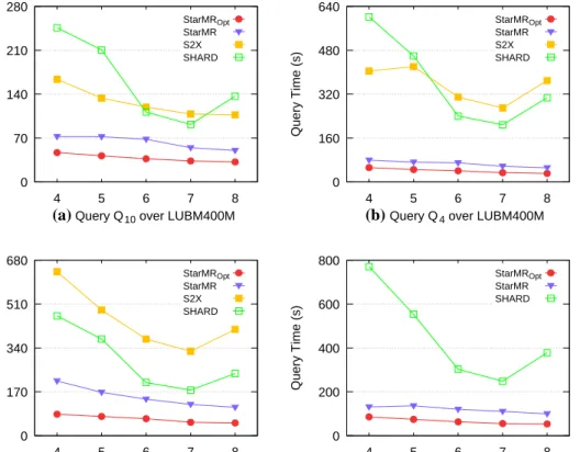
Similar to the previous scalability-examining experiments on the WatDiv datasets, we carried out extensive experiments on various size of LUBM datasets, i.e., LUBM4, LUBM40, and LUBM400. In addition, we verified the scalability of our methods by changing the number of sites. Furthermore, we selected four queries, Q4 , Q7 , Q9 , Q10 , which are covering all the query categories. The intuitive experimental results are shown in Figs. 9 and 10.
Different Size of Datasets We evaluated the scalability of the StarMRopt by changing the scale of LUBM data-sets. As shown in Fig. 9, the experimental results showed that the method we proposed significantly outperforms S2X and SHARD. We can observe that the query perfor-mance of all the queries decreased with the scale of datasets increasing. When S2X answers query Q9 over LUBM40 and
LUBM400, some errors occurred, which revealed that S2X cannot complete the query and often aborted. In contrast, the runtimes of our methods were significantly less than S2X and SHARD covering all queries. The average runtime of
StarMRopt covering all the query categories was about 18
seconds, which was up to 23 times faster than that of S2X,
and 13 times faster than that of SHARD. We analyze the reason can be that our optimization method exploited the structure features, semantic information, and heuristic algo-rithms, which can reduce the expensive overhead incurred by the intermediate results.
Different Numbers of Cluster Sites The scalability of each method was evaluated on LUBM400 dataset with the number of cluster sites varying from 4 to 8, as shown in Fig. 10. It was intuitive that for most queries, the runtimes decreased with the cluster sites increasing. We analyzed that
Fig. 10 Scalability on cluster cites 0 70 140 210 280 4 5 6 7 8 Query Time (s)
(a) Query Q10 over LUBM400M StarMROpt StarMR S2X SHARD 0 160 320 480 640 4 5 6 7 8 Query Time (s)
(b) Query Q4 over LUBM400M StarMROpt StarMR S2X SHARD 0 170 340 510 680 4 5 6 7 8 Query Time (s)
(c) Query Q7 over LUBM400M StarMROpt StarMR S2X SHARD 0 200 400 600 800 4 5 6 7 8 Query Time (s)
(d) Query Q9 over LUBM400M StarMROpt StarMR SHARD 100 101 102 103 104 L1 L2 S1 S2 F1 F2 C1 C2 Query Time (s) DBpedia StarMRopt StarMR S2X SHARD
more cluster sites generate more degree of parallelism so that there were more threads to execute query tasks. How-ever, the runtimes of S2X and SHARD decreased from 4 to 7, but increased from 7 to 8 instead. After an in-depth analysis, we concluded that when the parallelism number increased to a certain extent, the expensive communication cost became the bottleneck.
In addition, S2X cannot complete queries Q9 on all the
number of cluster sites, the result validated the conclusion that the performance of S2X cannot beat our methods. To summarize, our proposed methods achieved better perfor-mance than S2X and SHARD.
6.4 Experiments on the Real‑World Dataset
To evaluate the efficiency and scalability of StarMRopt on a real-world dataset DBpedia, extensive experiments were car-ried out. Our experimental results are shown in Figs. 11 and 12. More specifically, we compared our proposed methods with the close competitors, i.e., S2X and SHARD. On the one hand, we used the average runtimes to verify the effi-ciency; on the other hand, we changed the number of cluster sites to examine the scalability of these methods.
6.4.1 Efficiency on DBpedia
Extensive experiments were carried out to verify the query efficiency of our method on the real-world datasets DBpedia. Figure 11 compared the different algorithms over DBpedia covering all query categories.
We can observe that SHARD showed a good performance for all the query types over DBpedia dataset, for the rea-son that the query time of it tended to be more stable than S2X. But SHARD was not able to beat our methods for any query. As shown in Fig. 11, StarMRopt also demonstrated
the best query efficiency on all queries over DBpedia, and
StarMR performed much better than the other two methods, i.e., S2X and SHARD. When answering C2 , i.e., the query
Q1 mentioned in Sect. 1, S2X terminated with errors. Thus, S2X cannot efficiently evaluate the complex query involving a large number of intermediate results. For the remaining seven queries, the execution speeds in StarMRopt was about
4 to 469 times faster than that in S2X, and about 7 to 20 times faster than that in SHARD. Compared with StarMR,
the time of StarMRopt was reduced from 44.19% to 67.48%, i.e., the optimization effect on DBpedia was prominent. So in summary, the experimental results in Fig. 11 demonstrated that StarMRopt reduced invalid input data and postponed Cartesian product operations by a large margin.
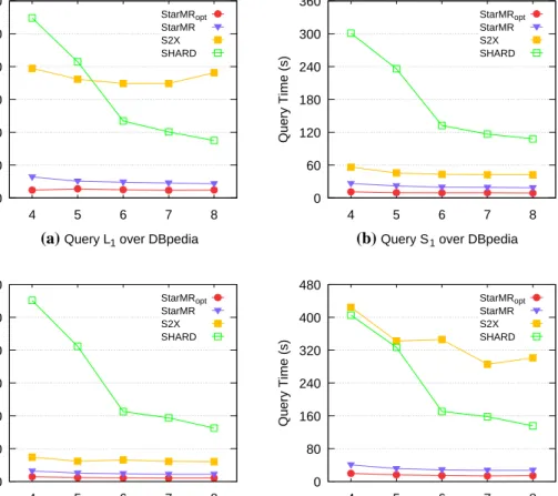
Fig. 12 Scalability on DBpedia
0 60 120 180 240 300 360 4 5 6 7 8 Query Time (s)
(a) Query L1 over DBpedia StarMRopt StarMR S2X SHARD 0 60 120 180 240 300 360 4 5 6 7 8 Query Time (s)
(b) Query S1 over DBpedia StarMRopt StarMR S2X SHARD 0 100 200 300 400 500 600 4 5 6 7 8 Query Time (s)
(c) Query F1 over DBpedia StarMRopt StarMR S2X SHARD 0 80 160 240 320 400 480 4 5 6 7 8 Query Time (s)
(d) Query C1 over DBpedia StarMRopt
StarMR S2X SHARD