A Deep Learning Framework for Optimization of MISO Downlink Beamforming

Kent Academic Repository

Full text document (pdf)

Copyright & reuse

Content in the Kent Academic Repository is made available for research purposes. Unless otherwise stated all content is protected by copyright and in the absence of an open licence (eg Creative Commons), permissions for further reuse of content should be sought from the publisher, author or other copyright holder.

Versions of research

The version in the Kent Academic Repository may differ from the final published version.

Users are advised to check http://kar.kent.ac.uk for the status of the paper. Users should always cite the published version of record.

Enquiries

For any further enquiries regarding the licence status of this document, please contact:

[email protected]

If you believe this document infringes copyright then please contact the KAR admin team with the take-down information provided at http://kar.kent.ac.uk/contact.html

Citation for published version

Xia, Wenchao and Zheng, Gan and Zhu, Yongxu and Zhang, Jun and Wang, Jiangzhou and Petropulu,

Athina P. (2019) A Deep Learning Framework for Optimization of MISO Downlink Beamforming.

IEEE Transactions on Communications . ISSN 0090-6778.

DOI

https://doi.org/10.1109/TCOMM.2019.2960361%E2%80%8B

Link to record in KAR

https://kar.kent.ac.uk/79640/

Document Version

Author's Accepted Manuscript

A Deep Learning Framework for Optimization

of MISO Downlink Beamforming

Wenchao Xia,

Student Member, IEEE,

Gan Zheng,

Senior Member, IEEE

,

Yongxu Zhu, Jun Zhang,

Member, IEEE,

Jiangzhou Wang,

Fellow, IEEE

, and

Athina P. Petropulu,

Fellow, IEEE

Abstract

Beamformingisaneffectivemeanstoimprovethequalityofthereceivedsignalsinmultiuser multiple-input-single-output (MISO) systems. This paper studies fast optimal downlink beamforming strategies by leveraging powerful deep learning techniques. Traditionally, finding the optimal beamforming solution relies on iterative algorithms which leads to high computational delay and is thus not suitable for real-time implementation. In this paper, weproposea deep learningframework forthe optimization of downlinkbeamforming.In particular, thesolutionisobtainedbasedonconvolutionalneuralnetworksandexploitationofexpertknowledge,suchasthe uplink-downlinkduality and the knownstructureof optimal solutions.Using this framework,we constructthree beamformingneuralnetworks(BNNs)forthreetypicaloptimizationproblems,i.e.,the signal-to-interference-plus-noiseratio(SINR)balancing problem,the powerminimizationproblem andthe sumrate maximizationproblem. The BNNs for the former two problems adopt the supervised learning approach, while the BNN for the sum rate maximization problem employs a hybrid method of supervised and unsupervised learning to improve the performance. Simulationresults show that withmuch reducedcomputationalcomplexity, the BNNscanachieve near-optimalsolutionsto theSINRbalancing and powerminimizationproblems, andcanachieve aperformance closetothat ofthe weightedminimum meansquarederroralgorithm forthesum ratemaximization problem.In summary,thisworkpavesthewayforfast realizationofoptimalbeamforminginmultiuserMISOsystems.

Index Terms

Deep learning, beamforming, MISO, beamforming neural network.

W. Xia and J. Zhang are with the Jiangsu Key Laboratory of Wireless Communications, Nanjing University of Posts and Telecommunications, Nanjing 210003, China (e-mail: [email protected], [email protected]).

G. Zheng and Y. Zhu are with the Wolfson School of Mechanical, Electrical and Manufacturing Engineering, Loughborough University, Leicestershire, LE11 3TU, UK (e-mail: [email protected], [email protected]).

J. Wang is with the School of Engineering and Digital Arts at the University of Kent, Kent, CT2 7NT, UK (e-mail: [email protected]).

A. P. Petropulu is with the Department of Electrical & Computer Engineering Rutgers, The State University of New Jersey, Piscataway, NJ 08854 (e-mail: [email protected]).

I. INTRODUCTION

Downlink beamforming techniques have attracted much attention in the past decades for its ability to realize the performance gain of the multiple antennas. Beamforming has been formulated in various ways, i.e., as a signal-to-interference-plus-noise ratio (SINR) balancing problem (also known as interference balancing problem) under a total power constraint [2–4], as a power minimization problem under quality of service (QoS) constraints [5–8], or as a sum rate maximization problem under a total power constraint [2, 9–11]. Existing approaches to finding the optimal beamforming solutions heavily rely on tailor-made iterative algorithms and convex optimization, which is in turn solved by general iterative algorithms such as the interior point method. For instance, the SINR balancing problem can be solved by the iterative algorithm of [12]. The power minimization problem can be reformulated as a second-order cone programming (SOCP) [7, 8] or semidefinite programming (SDP) problem [13, 14], which can be solved directly by an optimization software package such as CVX [15]. Its optimal solution can also be obtained using iterative algorithms such as Algorithm A of [16] and the dual algorithm of [5, 12]. However, the optimal solution to the sum rate maximization problem is usually hard to obtain because the problem is nonconvex. Locally optimal solutions are obtained via iterative algorithms, such as the weighted minimum mean squared error (WMMSE) algorithm [9, 10], and asymptotically optimal solutions are obtained using the water filling algorithm combined with zero-forcing (ZF) beamforming [11].

The main drawbacks of existing iterative algorithms are the high computational complexity and the resulting latency. As a result, the beamforming technique is unable to meet the demands of real-time applications in the fifth-generation (5G) system and beyond, such as autonomous vehicles and mission critical communications. Even in non-real-time applications, where the small-scale fading varies in the order of milliseconds, the latency introduced by the iterative process renders the beamforming solution outdated. To address this challenge, researchers have proposed some simple heuristic beamforming solutions which admit closed-form solutions, such as the maximum-ratio transmission beamforming, the ZF beamforming, and the regularized ZF (RZF) beamforming. These heuristic beamforming solutions are directly computed based on the channel state information (CSI) without iteration, and thus involve low computational delay. However, the reduction of delay is achieved at the cost of performance loss. The tradeoff

between delay and performance seems to restrict the potential of the beamforming techniques

and its applications in practice.

Thanks to the recent advances in deep learning (DL) techniques, it becomes possible to find

the optimal beamforming in real time by taking into account both the performance and the

computational delay simultaneously. This is because the DL technique trains neural networks

offline and then deploysthe trained neural networks for onlineoptimization. Thecomputational

complexity is transferred from the online optimization to the offline training, and only simple

linear and nonlinear operations are needed when the trained neural network is used to find the

optimal beamforming solution, thus greatly reducing the computational complexity and delay.

Benefiting from the development of specialized hardware, such as graphic processing units

and field programmable gate arrays, DL can be implemented using these hardware resources

conveniently. Accordingly, DL techniques have been widely used in many applications

includ-ing wireless communications. A lot of research has attempted to use DL to deal with some

issues in the physical layer, including channel decoding [17,18], detection [19–21], channel

estimation [22–24], and resource management [25–32]. Among these efforts, the autoencoder

basedonunsupervisedDL,investigatedin[33,34],isanambitiousattempttolearnanend-to-end

communications system [35]. DL can also facilitate resource management [25,26], e.g. power

allocation [27–31]. Finally, [36,37] provide an overview on the recent advances in DL-based

physical layer communications and [38] suggests potential applications of DL to the physical

layer.

However, with the exception of [39–42], there are no works focusing on the beamforming

design in multi-antenna communications based on DL. A common method used in the already

published papers is codebook-basedbeam selection. For example, [39] designeda decentralized

robustprecoding schemebased onDNN ina networkMIMO configuration.The projectionover

a finite dimensional subspace in [39] reduced the difficulty, but also limited the performance.

[40]usedaDLmodeltopredictthebeamformingmatrixdirectlyfromthesignalsreceivedatthe

distributed BSs based on omni or quasi-omni beam patterns in millimeter wave systems, whose

sum rate performance was restricted by the quantized codebook constraint. [39,40] predicted

the beamforming matrix in the finite solution space at the cost of performance loss. Different

from[39,40],[41,42]directlyestimatedthebeamformingmatrixwithoutexploitingtheproblem

transmit antennas and users increase. This will lead to high training complexity of the neural

networks when the numbers of transmit antennas and users are large. Furthermore, we notice

that none of them addressed the SINR balancing problem under a total power constraint and

power minimization problem under SINR constraints.

Motivated by the aforementioned facts and the universal approximation theorem [43,44], we

propose a general DL framework to achieve not only near-optimal beamforming matrix, but

alsoreduce complexityandlatencyas comparedtotheiterative methods.Based ontheproposed

framework, wedevelopbeamformingneuralnetworks(BNNs)to solvethethree aforementioned

optimization problems. Learning the optimal beamforming solution is highly nontrivial, and

there are still challenges that need to be addressed in designing the BNNs. Firstly, the popular

neural network softwarepackages such as Keras and Tensorflow currently (March2019) do not

support complex numbers as input or output [35]. Both channel and beamforming vectors are

inherently complex. Naive transformation of complex beamforming vectors to real vectors by

concatenating the real and imaginary parts and predicting the real beamformingvectors directly

not only lead to high complexity of prediction, but also may lose the specific structures of the

problems of interest. Secondly, the power minimization problem has strict QoS constraints and

guaranteeinga feasible solutionusing neuralnetworks isa challenge. In addition, differentfrom

the SINR balancing problem and power minimization problem, there is no practically useful

algorithm that can achieve the optimal solution to the sum rate maximization problem (and

other nonconvex beamforming problems), and thus the supervised learning method based on

locally optimal solution cannot achieve good performance. In this paper, we will tackle these

challenges, and our main contributions are summarized as follows:

• We provide a DL-based framework for the beamforming optimization in the

multiple-input-single-output (MISO) downlink, where the BS has multiple antennas while each user terminal has a single antenna. The proposed framework is designed based on the CNN structure. Different from existing works where the CNN was applied to power control [29, 30], resource allocation [45], and wireless scheduling [46], the proposed framework combines the signal processing module with the neural network module and exploits expert knowledge such as the uplink-downlink duality and the known structure of optimal solutions, so as to improve learning efficiency by specifying the best parameters to be learned; those parameters are typically not the direct beamforming matrix. This framework can deal with

threetypesofbeamformingoptimizationproblems:1)problemswhoseoptimalsolutionsare

easy to find and the constraints are easy to meet; 2) problems whose optimal solutions are

easyto findbut theconstraintsarehard tomeet;and 3)problemswhich havenopractically

useful algorithm that can achieve optimal solutions efficiently. Under this framework, we

propose three BNNs for solving three typical optimization problems in MISO systems,

i.e., the SINR balancing problem under a total power constraint, the power minimization

problemunderQoSconstraints, andthesumratemaximizationproblemunderatotalpower

constraint.

• IntheproposedsupervisedBNNsfortheSINRbalancingproblemandthepower

minimiza-tion problem, instead of estimating the beamforming matrix with N K elements, where N

is the numberof the transmit antennasat the BS andK is the number ofusers, weexploit

the uplink-downlink duality of solutions [5,6,12] and predict the virtual uplink power

allocation vector with only K elements. Thus, the demand on the prediction capability

of the BNNs in terms of network neurons and layers is significantly reduced. Also, the

training andprediction complexityand cost arereduced. In the proposedBNN for thesum

ratemaximizationproblem, weexploittheknownstructureof optimalsolutionsandpredict

two power allocation vectors with totally 2K elements. This approach still has advantages

compared to predicting the beamforming matrix directly.

• Weproposeahybridtwo-stageBNNwithbothsupervisedandunsupervisedlearningtofind

the beamforming solution to the sum rate maximizationproblem [29], since no practically

useful algorithm can find the global optimum. In the first stage, we use the supervised

learning method with the mean squared error (MSE)-based loss function to make the

predictions as close as possible to the WMMSE algorithm, which is known to achieve the

locally optimal solution. In the second stage, we modify the metric in the loss function to

be thesum rate, andupdate the networkparametersaccording tothe unsupervisedlearning

method, which achieves a performance close to that of the WMMSE algorithm.

The remainder of this paper is organized as follows. Section II introduces the system model and formulates three beamforming optimization problems in the MISO downlink. Section III provides the framework for the beamforming optimization and then Sections IV, V and VI propose the BNNs under the framework for the SINR balancing problem, the power minimization problem,

and the sum rate maximization problem, respectively. Numerical results are presented in Section VII. Finally, conclusion is drawn in Section VIII.

Notations:The notations are given as follows. Matrices and vectors are denoted by bold capital

and lowercase symbols, respectively.(A)T and(A)H stand for transpose and conjugate transpose

of A, respectively. The notations || • ||1 and || • ||2 are l1 and l2 norm operators, respectively.

The operator diag(a)denotes the operation to diagonalize the vectorainto a matrix whose main

diagonal elements are from a. Finally, a ∼ CN(0,Σ) represents a complex Gaussian vector

with zero-mean and covariance matrix Σ.

II. SYSTEMMODEL

We consider a downlink transmission scenario where a BS equipped with N antennas serves

K single-antenna users. The channel between userk and the BS is denoted ashk∈_CN×1 _{. The}

received signal at user k is given by

yk =hHk

K

X

k0₌₁

wk0x_k0 +n_k, (1)

wherewkrepresents the beamforming vector for userk,xk ∼ CN(0,1)is the transmitted symbol

from the BS to userk, and nk ∼ CN(0, σ2)denotes the additive Gaussian white noise (AWGN)

with zero mean and variance σ2_{. The received SINR of user k equals}

γ_kdl = |h H kwk|2 PK k0_=1,k0_6=k|hH_kwk0|2+σ2 . (2)

One conventional optimization problem seeks to maximize minkγkdl/ρk subject to a transmit

power constraint, where ρk’s are constant weights denoting the importance of the sub-streams.

Such an optimization problem is referred to as interference or SINR balancing, and has been investigated in many works [2–4]. The SINR balancing problem is formulated as:

P1: max W 1≤mink≤K γdl k ρk , s.t. K X k=1 ||wk||2 ≤Pmax, (3)

where W= [w1,w2, . . . ,wK] is a set of beamforming vectors and Pmax is the power budget.

Another important problem is the power minimization problem under a set of SINR constraints [6, 7]. A network operator may be more interested in how to minimize the transmit power while fulfilling the demands for QoS, i.e.,

P2: min W K X k=1 ||wk||2, s.t. γkdl ≥Γk,∀k, (4)

whereΓkistheSINRconstraintofuserk.Foreaseofreference,wedefineΓ=[Γ1,···,ΓK]Tas

theSINRconstraintvector.

Finally, the weighted sum rate maximization problem under the power constraint is also an

important issue that has attracted lots of attention [2,9,10], which can be formulated as:

P3: max W K X k=1 αklog2(1 +γ dl k), s.t. K X k=1 ||wk||2 ≤Pmax, (5)

whereαkisaconstantweightofuserk.

We choose theabove problemsas representativeexamplesto demonstratethe effectivenessof

our proposed DL beamforming framework. The practical algorithms to find optimal solutions

are availablefor P1 [8,12,47] andP2 [5,7,8,12,13], sosupervised learning canbe adopted. In

thiswork, forsimplicity,weassumetheoptimalsolutionto problemP2alwaysexistsanddonot

consider the infeasibility of QoS constraints. Under this assumption, P2 still has the additional

challenge of satisfying the strict QoS constraints. P3 is a difficult nonconvex problem and is

usually solved using the iterative WMMSE approach [9,10], therefore supervised learning is

insufficient and further improvement is needed. In the rest of the paper, we will show how the

solutions to these three types of problems can be efficiently learned by the proposed DL-based

beamforming framework.

III. ADL-BASEDFRAMEWORK FORBEAMFORMINGOPTIMIZATION

DL-basedneuralnetworkswere initiallydesignedforsolvingclassificationproblems, butthey

can also achieve satisfactory performance in regression problems. For example, the DNN was

used to predict transmit power [27,28]. Existing works mainly take real data, such as channel

gains and transmit power, as input and output, but channel and beamforming matrices are both

complex.Inaddition, predictingthebeamformingmatrixwithN K elementsdirectlymayleadto

inaccurateand evenunder-fittingresults. Obviouslywe canuse wideror deeperneuralnetworks

with more neurons to improve the learning ability, but such a huge network will lead to high

training and implementation complexities and cannot guarantee the learning performance. For

MSE/MAE CL AC CL AC FC AC BN Output Flatten BN Input

Neural network module

I(h)

R(h)

Supervised/ unsupervised learning

Beamforming recovery module

Key

features Beamforming _matrix

...

...

Expert knowledge

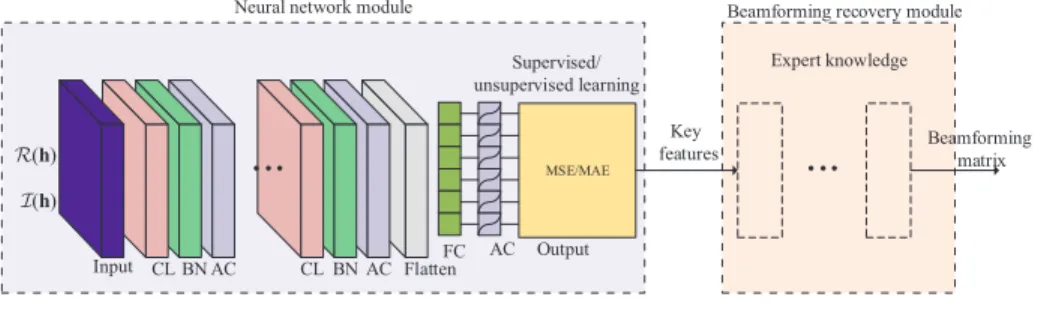
Fig. 1. A DL-based framework for the beamforming optimization in MISO downlink, which includes two main modules: the neural network module and the beamforming recovery module. The neural network module is composed of an input layer, convolutional (CL) layers, batch normalization (BN) layers, activation (AC) layers, a flatten layer, a fully-connected (FC) layer, and an output layer, whereas the key features and the functional layers in the beamforming recovery module are specified by the expert knowledge.

The proposed DL-based framework for the beamforming optimization in MISO downlink is shown in Fig. 1. We choose the CNN architecture as the base of the framework, because the CNN has strong ability of extracting features. In addition, the CNN can reduce the number of learned parameters by sharing weights and biases [30]. The CNN has a lot of applications in wireless networks, such as power control [29, 30], resource allocation [45], and wireless scheduling [46]. To overcome the challenge of predicting the beamforming matrix directly, we take the expert knowledge of the beamforming matrix into account. The proposed framework, instead of estimating the beamforming matrix directly, only predicts the key features extracted from the beamforming matrix according to the expert knowledge specific to the problem of interest. Therefore the demand for the prediction capability of the BNNs in terms of network neurons and layers, as well as the complexity, is significantly reduced.

A. Structure of the Proposed Framework

The proposed framework includes two main modules: the neural network module and

beam-forming recovery module. The neural network module is composed of an input layer,

convo-lutional layers, batch normalization layers, activation layers, a flatten layer, a fully-connected

layer, and an output layer, whereas key features and the functional layers in the beamforming

recovery module are specified by the expert knowledge. For ease of clarification, we assume

that, besides the input, output, flatten, and fully-connected layers, there are L = |L| groups of

functional layers in the neural network module and each group includes a convolutional layer,

layers.

1) Input Layer: The complex channel coefficients are fed into the neural network module

to predict the key features, which are not supported by the current neural network software. To deal with this issue, two data transformations are available. One is to separate the complex

channel vector, for example h = [hT

1,· · ·,hTK]T ∈ CN K

×1_{, into the in-phase component R(h)}

and quadrature component I(h), where R(h) and I(h) contain the real and imaginary parts

of each element in h, respectively. We call this transformation I/Q transformation. Another

transformation, suggestedby [48], isto mapthe complex channelvectorh into tworealvectors

P(hk) and M(hk), where the former contains the phase information and the latter includes the

magnitudeinformationofh.ThistransformationisreferredtoasP/Mtransformation.Asfaras

weknow,thereisnoevidencetoshowwhichtransformationisbetter.Inthiswork,weadoptI/Q

transformation of complex channels and formulate the input of the first convolutional layer as [R(h),I(h)]T_∈

R2×N K.Notethatthesamplesarefedintotheneuralnetworkmoduleinbatches

duringthetrainingprocess.

2) Convolutional Layer: Each convolutional layerl∈ L createscl convolution kernels of size

al×al that are convolved with the layer input Iconv,l ∈Rb

(1) l−1×b (2) l−1×cl−1_{, where b}(1) l−1 and b (2) l−1 are

the height and width of the output of the convolutional layerl−1, respectively. Note thatc0 = 1

b(1)₀ = 2, and b(2)₀ = N K. The parameters of the convolution kernels, including the weights

Ξl ∈ Ral×al×cl and a bias vector ξl ∈ Rcl×1, are shared among different elements in Iconv,l to

extract features. More specifically, the output Oconv,l ∈ Rb

(1)

l ×b

(2)

l ×cl _{of the convolutional layer l}

is

Oconv,l =Conv(Iconv,l,Ξl,ξl), l∈ L, (6)

where the operator Conv(·,·,·) denotes the convolution operation.

3) Batch Normalization Layer: The batch normalization layers are introduced in the neural

networkmodule,whichcanbeputbeforeoraftertheactivationlayers[49]accordingtopractical

experience.Intheproposedframework,weadopttheformerwherethebatchnormalizationlayers

normalizetheoutputoftheconvolutionallayersthroughsubtractingthebatchmeananddividing

by the batch standard deviation, i.e.,

Zbn,l,c[i, j] = Oconv,l,c[i, j]−µl,c p Varl,c+l,c , l∈ L, c= 1,· · · , cl, i= 1,· · · , b (1) l , j = 1,· · · , b (2) l (7)

where X[i, j] denotes (i, j)-th element of matrix X, Oconv,l,c ∈ Rb (1) l ×b (2) l is the c-th slice of Oconv,l,µl,c = PF f=1 Pb (1) l i=1 Pb (2) l j=1O (f) conv,l,c[i,j] F b(1)_l b(2)_l and Varl,c = PF f=1 Pb (1) l i=1 Pb (2) l j=1 O (f) conv,l,c[i,j]−µl,c 2

F b(1)_l b(2)_l arethebatch

meanandvarianceofthec-thslice,respectively,l,cisasmallfloataddedtothevariancetoavoid

dividing by zero, and F is the batch size. Note that such a simple normalization process may

changewhatthelayercanrepresent.Toaddressthisissue,twotrainableparametersθl,candβl,care

introducedtoscaleandshiftthenormalizedvalueZbn,l,c[i,j]asZˆbn,l,c[i,j]=βl,cZbn,l,c[i,j]+θl,c.

This “denormalization” process is allowed by changing only these two parameters, instead of

changingallparameterswhichmayleadtotheinstabilityoftheneuralnetworkmodule. Besides,

the work in [49] claimed that the batch normalization layer can reduce the probability of

over-fitting, enable a higher learning rate, and make the neural network less sensitive to the

initializationofweights.Notethatthebatchnormalizationlayersareelement-wisefunctions,such

thattheydonotchangetheirrespectiveinputshapes.

4) Activation Layer: Since the predicted variables are continuous and positive real numbers,

it is suggested that the activation functions that can generate negative values, such as tanh and

linear functions, should not be usedin the last activation layer. The rectified linearunit (ReLU)

and sigmoid functions are good choices for the last activation layer, which are given as

ReLU(z) = max(0, z) and sigmoid(z) = 1

1 +e−z, (8)

respectively. The most common choice for the intermediate activation layers is the ReLU func-tion. Note that the functions performed in the activation layers are element-wise functions, such that their outputs have the same shapes of their inputs, respectively.

5) Flatten Layer, Fully-connected Layer, and Output Layer: The flatten layer is only used to

change the shape of its input into a vector, for the fully-connected layer to interpret. The output

ofc ∈Rm×1 of the fully-connected layer is

ofc =Πifc+π, (9)

whereifc ∈R2N KcL×1 is the input vector,Π∈Rm×2N KcL andπ ∈Rm×1 account for the weight

matrix and bias vector, respectively, and m is the number of the neurons in the fully-connected

layer. The main function of the output layer is to generate the predicted results after the neural network finishes training.

Note that apart from these functional layers, the loss function also plays an important role in the proposed framework, which is marked on the output layer in Fig. 1. The loss function

together with the learning rate guides the learning process of the neural network. In other words, the loss function “tells” the neural network how to update its parameters. Since the output values are continuous, it is suggested to utilize the mean absolute error (MAE) or the MSE as a metric.

Given the predicted results of the f-th sample in the neural network module is qˆ(f) _{and the}

target result is q(f)_{, the MAE and MSE are defined as}

MAE= 1 F K F X f=1 ||q(f)−qˆ(f)||1 and MSE= 1 F K F X f=1 ||q(f)−qˆ(f)||2 2, (10)

respectively.Generallyspeaking,theMAEfunctionismorerobustandisnotaffectedbyoutliers.

On the contrary, the MSE loss function is highly sensitive to outliers in the dataset because the

MSE functiontries toadjust the modelaccording tothese outlier values, atthe expense ofother

samples [50]. In this work, the training dataset is generated by simulationsand outliers are not

an issue. Then we choose the MSE as the loss metric because its gradient is easier to calculate

than that of the MAE.

6) Beamforming RecoveryModule: The beamformingrecovery module is an important

com-ponent whose aim is to recover the beamforming matrix from the predicted key features at

the output layer. The functional layers in the beamforming recovery module are designed

ac-cording to the expert knowledgeof the beamforming optimization which maps/convertsthe key

features to the beamforming matrix. The expert knowledge is problem-dependent and has no

unified form, but what is in common is that the expert knowledge can significantly reduce the

number of variables to be predicted compared to the beamforming matrix. For example, the

uplink-downlink duality and specific solution structures are the typical expert knowledge for

beamforming optimization.

Thekeyfeaturesshouldbechosencarefullytomeetsomeconstraintsrequiredbyapplyingthe

universal approximation theorem [27, 43], so that a feedforward network exists which can

approximate the continuous mapping from the channel coefficients to the key features. More

specifically, assume that τ is a vector containing the chosen key features, the mapping function

f(•)fromhtoτ,i.e., τ=f(h),shouldbeareal-valuedcontinuousfunctionoveracompactset.

The compact set requirement holds whenever the possible values of the input h are bounded.

However,thecontinuityofthemappingfunctiondependsonthechoiceofthekeyfeatures.

InnextthreesectionswewillproposethreeBNNsundertheproposedframeworkforproblems

the expert knowledge and choose the key features.

B. Computational Complexity

The computational complexity of the proposed framework involves two main tasks: the online prediction and the offline training. To the best of our knowledge, complexity analysis of the offline training is still an open issue mainly because of the complex implementation of the backpropagation process. However, since the training is performed offline, and updated at a much longer time-scale compared to the online prediction, we assume its complexity can be afforded [51]. Thus, we focus on the complexity of the online prediction. In addition, the functional layers are problem-dependent in the beamforming recovery module, so only the complexity of the neural network module is analyzed below.

Given there are cl kernels of size al×al in the l-th convolutional layer, then the numbers

of multiplication and addition operations of convolutional layer l are the same and equal to

a2_lb(1)_l b(2)_l cl−1cl. Thus, the total time complexity of all convolutional layers measured by the

num-ber of multiplications isOP l∈La2lb (1) l b (2) l cl−1cl

[52]. It is known that the batch normalization layers and activation layers are element-wise functions, thus the computational complexity of

total batch normalization layers and total activation layers in L groups is OP

l∈Lb (1) l b (2) l cl . The numbers of multiplication and addition operations of the fully-connected layer are also the

same and equal tob(1)_L b(2)_L cLm, respectively. Then the time complexity of the fully-connected layer

is given as Ob(1)_L b(2)_L cLm

. Besides, the complexity of the input, output, and flatten layers are ignored due to the simplicity of their functions. If all convolutional layers use the kernels of size

3×3 and apply stride 1 and zero padding 1, thenb(1)_l = 2 andb(2)_l =N K,∀l ∈ L. Based on the

above analysis and assuming the parameters of the neural network module are fixed, predicting

the output of the neural network module needs 2N KP

l∈L(9clcl−1 +cl) + 2N KcLm + 2m

arithmetic operations including multiplications, divisions, and exponentiations, and has an

ap-proximate complexity O(N K).

IV. BNNFORSINR BALANCINGPROBLEM

As mentioned above, estimating the beamforming matrix directly leads to the higher com-plexity of prediction due to the large amount of variables. In order to reduce the prediction complexity, we introduce a scheme which first predicts the power allocation vector as the key

feature and then achieves the corresponding beamforming matrix based on the predicted results. Such a scheme is based on the expert knowledge named the uplink-downlink duality.

A. Uplink-Downlink Duality

Before we present the BNN for the SINR balancing problem P1, we first introduce the

following lemma to describe the uplink-downlink duality of problem P1 [12].

Lemma 1. Given W˜ = [ ˜w1,w˜2, . . . ,w˜K] and Pmax, we have

Cdl( ˜W, Pmax) =Cul( ˜W, Pmax), (11)

where Cdl_{( ˜W, P}

max) and Cul( ˜W, Pmax) are given as

Cdl( ˜W, Pmax) = max p 1≤mink≤K γdl k ( ˜W,p) ρk (12) s.t. ||p||1 ≤Pmax, ||wk˜ ||2 = 1,∀k, and Cul( ˜W, Pmax) = max q 1≤mink≤K γ_kul( ˜W,q) ρk (13) s.t. ||q||1 ≤Pmax, ||w˜k||2 = 1,∀k, respectively, with γ_kdl( ˜W,p) = pk|h H kw˜k|2 PK k0_=1,k0_6=kpk0|hH kw˜k0|2+σ2 , (14) and γ_kul( ˜W,q) = qk|h H kw˜k|2 PK k0_=1,k0_6=kqk0|hH k0w˜k|2+σ2 . (15)

Note that p = [p1, . . . , pK]T and q = [q1, . . . , qK]T are downlink and uplink power vectors,

respectively1.

Note that problem (12) is an equivalent virtual problem of problemP1whose optimal solutions

are connected by W∗ = ˜W∗P∗ where P∗ =diag(p∗), W∗ is the optimal solution to problem

1

P1, andW˜ ∗ andp∗ are the optimal solutions to problem (12). Based onLemma 1, we find that the uplink and downlink scenarios have the same achievable SINR region and the normalized beamforming designed for the uplink reception immediately carries over to the downlink

trans-mission [12]. Thus we first obtain the optimal power allocationq∗ and beamforming matrix W˜ ∗

for the easier-to-solve uplink problem (13) instead of the downlink problem (12). Then given the

optimal beamformingW˜ ∗, the optimalp∗ is obtained as the firstK components of the dominant

eigenvector of the following matrix [53]

Υ( ˜W∗, Pmax) =   DU Dσ 1 Pmax1 T_DU 1 Pmax1 T_Dσ  , (16) where σ = σ2_{1, 1 = [1,1, . . . ,1]}T _∈ RK×1, D = diag{ρ1/|( ˜w∗1)Hh1|2, . . . , ρK/|( ˜w∗K)HhK|2}, and [U]kk0 =      |( ˜w∗_k0)Hh_k|2, if k0 6=k, 0, else. (17)

Finally, the downlink beamforming matrix is derived asW∗ = ˜W∗P∗. Thus, instead of predicting

W directly, we can predict the uplink power allocation vector q. In the supervised learning

method, the prediction performance of the BNN depends on the quality of training samples. To

generate the training samples, the optimal q∗ and W˜ ∗ can be found by an iterative optimization

algorithm in [12, Table 1].

Note that Υ( ˜W∗, Pmax) is a non-negative matrix and the optimal objective value of problem

P1 is the reciprocal of the largest eigenvalue of Υ( ˜W∗, Pmax) [53]. According to the

Perron-Frobenius theory, for any nonnegative real matrix Ω with spectral radius χ(Ω), there exist a

vectorδ ≥0such that Ωδ =χ(Ω)δ [54]. Based on [12, Theorem 3], the sequence of the target

value of problem P1 provided by the iterative algorithm in [12, Table 1] is strictly

monotoni-cally increasing and the largest eigenvalue of Υ( ˜W∗, Pmax) is unique. Then the corresponding

eigenvector containing q is a continuous and bounded function of h according to [55, Chapter

3]. Thus, we can use a neural network to approximate the mapping function from h to q [43].

B. BNN Structure

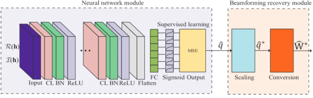
The proposed BNN for problemP1, shown in Fig. 2, is based on the proposed BNN framework

in Fig. 1. The functions and operations of the basic layers such as the input, convolutional, batch normalization, and output layers, are the same as those in the proposed framework. Therefore,

MSE CL ReLU CL ReLU FC Sigmoid BN Conversion Output Flatten BN Input

Neural network module

Scaling ݍො ݍොכ I(h) R(h) ෡כ Supervised learning

...

Beamforming recovery module

Fig.2. BNNfortheSINRbalancingproblem.

we do not explain these layers here and readers can refer to Section III for detail. Note that in

theproposedBNNforproblemP1, theintermediateactivationlayersarefulfilledwiththeReLU

functionwhereasthelastactivationlayeris implementedusingthe sigmoidfunction.Besidesthe

existing layers in the framework, a scaling layer and a conversion layer are also introduced in

the BNN for problemP1, which belongto the beamforming recovery module. In the following,

we give the details of the scaling layer and the conversion layer.

1)ScalingLayer: Duetothe existenceofpredictionerror, itis almostimpossibletoguarantee

thattheoutputoftheoutputlayeralwaysmeetsthepowerconstraintinproblemP1. Accordingto

[56], the optimal solution is achieved when the equality of the constraint in problem P1 holds.

Therefore,wescaletheresultsoftheoutputlayerqˆtomeetthepowerconstraintbythefollowing

transformation, ˆ q∗ = Pmax ||qˆ||1 ˆ q. (18)

2) Conversion Layer: After receiving the scaled power allocation vector qˆ∗, we can achieve

the downlink beamforming matrix Wˆ ∗ as the final output of the BNN based on qˆ∗ by the

conversion layer. The beamforming recovery implemented by the conversion layer includes the following process: 1) Calculate T∗ =σ2_I N +PK_k=1qˆk∗hkhHk. 2) Calculate w˜∗_k = ˜w∗_k/||w˜∗_k||2,∀k, where w˜∗k = (T ∗ )−1hk.

3) Find the maximal eigenvalue ψ∗_max of Υ( ˜W∗, Pmax) and the associated eigenvector with

respect to ψ_max∗ , i.e., Υ( ˜W∗, Pmax)

_pˆ∗ 1 =ψ(maxi) _pˆ∗ 1 .

4) Output Wˆ ∗ = ˜W∗Pˆ∗ as the final result where Pˆ∗ =diag(ˆp∗).

Note that the time complexity of the beamforming recovery module is O(KN2_+N3_+K3_).

function based on the MSE metric is adopted.

V. BNNFORPOWER MINIMIZATIONPROBLEM

Similar to the BNN for the SINR balancing problemP1, the BNN for the power minimization

problemP2obtains the downlink beamforming matrix according to the uplink-downlink duality,

i.e., the expert knowledge. Specifically, we first predict the uplink power allocation vector as the key features using the trained neural network, then obtain the normalized beamforming matrix based on the predicted results. Finally, the downlink beamforming matrix is recovered from the normalized beamforming matrix by the uplink-downlink conversion method.

A. Uplink-Downlink Duality

Note that the conversion method adopted in the BNN for problem P1 can not be used again,

because the power budget Pmax is unknown in the power minimization problem P2. Instead, we

employ the conversion method in the following lemma [47].

Lemma 2. Given the optimal beamforming matrixW˜ ∗ = [ ˜w₁∗, . . . ,w˜∗_K]for the uplink problem2, i.e., min q,W˜ K X k=1 qk s.t. γ_kul( ˜W,q)≥Γk, ||w˜k||2 = 1,∀k, (19) where γ_kul( ˜W,q) is given as in (15).

The optimal beamforming vectors w∗_k,∀k, for the downlink problem P2, can be obtained

by multiplying the optimal normalized beamforming vector w˜_k∗ by a scaling factor, i.e., w_k∗ =

p∗_kw˜∗_k,∀k, where p∗_k is the k-th element of vector p∗ = [p∗₁, . . . , p∗_K]T _∈

RK×1 and

p∗ =σ2Ψ−11, (20)

2_{In this work, for simplicity, we assume the solution to problemP2always exists. However, it can happen that the wireless}

network only satisfies some of the users and thus the user selection is needed. To address this issue, a possible solution is to train another neural network for user selection, and then optimize the beamforming matrix among the selected users.

MSE CL ReLU CL ReLU FC Sigmoid BN Conversion Output Flatten BN Input

Neural network module

I_(h)

R(h)

ݍොכ ෡כ

Supervised learning

...

Beamforming recovery module

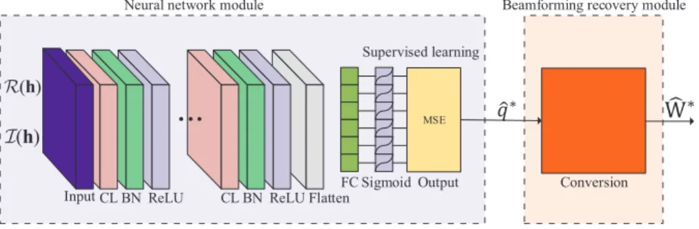
Fig. 3. BNN for the power minimization problem.

where [Ψ]kk0 =      1 Γk|h H kw˜ ∗ k|2, if k=k 0_, −|hH kw˜ ∗ k0|2, else. (21)

The vector p∗ of the scaling factors is the optimal downlink power allocation vector. Given

the optimal normalized beamforming matrix W˜ ∗, Lemma 2 allows us to achieve the optimal

downlink power vector p∗ by (20), then W∗ = ˜W∗P∗. Actually, if we know the uplink power

allocation vector q, the normalized beamforming matrix W˜ can be inferred as

˜ wk = T −1_hk ||T−1_h k||2 ,∀k, (22) where T =σ2_I

N +PK_k=1qkhkhHk. Therefore, the only results that need to be predicted by the

BNN is the uplink power allocation vector q, which reduces significantly the computational

complexity compared to the strategy that attempts to predict the beamforming matrix directly.

The iterative algorithm in [5] provides a way to achieve the optimal q∗ as the training samples

in the supervised learning method. Besides, such an iterative algorithm suggests the mapping

function from h to q is continuous [27, Theorem 1], so it can be approximated by a neural

network.

B. BNN Structure

The BNN for problem P2 in Fig. 3 is also based on the proposed BNN framework. However,

the operations of the conversion layer in Fig. 3 are different from those in the BNN for problem

P1. After receiving the uplink power allocation vectorˆq∗ from the output layer, the beamforming

recovery in the conversion layer performs the following operations:

1) Calculate T∗ =σ2IN +

PK

k=1qˆ ∗

2) Calculate w˜∗_k = ˜w∗_k/||w˜∗_k||2,∀k, where w˜∗k = (T

∗₎−1_h

k.

3) Calculate the downlink power allocation vector pˆ∗ =σ2(Ψ∗( ˜W∗,Γ))−11.

4) Output the downlink beamforming vectors wˆ∗_k= ˆp_k∗w˜∗_k,∀k, as the final results.

Here, the time complexity of the beamforming recovery module is O(KN2_+N3_+K3_{). Note}

that the predicted power vector qˆ∗ by the BNN is, in general, not exact. The prediction error

will lead to the inaccuracy of power allocation vector pˆ∗ as well as the downlink beamforming

ˆ

W∗. More specifically, if the predicted power vector qˆ∗ has an acceptable accuracy with respect

to the target power vector q∗, i.e., ||q∗ −qˆ∗||2

2 < ε where ε is a small constant, then we can

obtain a suboptimal solution whose objective value is larger than that of the optimal solution, i.e.,

PK k=1||wˆ ∗ k||22 > PK k=1||w ∗

k||22. Intuitively, the extra power consumption qextra =

PK k=1||wˆ ∗ k||22− PK k=1||w ∗

k||22 can be regarded as the cost of the prediction error. However, if the predicted vector

2 2

qˆ∗hasa significant error, i.e., ||q∗−qˆ∗|| ε, the downlinkbeamforming Wˆ ∗inferredfrom the

prediction qˆ∗may becomeinfeasible sincesome elements ofthe vector pˆ∗havenegative values.

This suggeststhat differentfromproblem P1, there isa certainprobability ofinfeasibility ofthe

BNNpredictionforproblemP2.However,ourexperimentsshowthatthefailureprobabilityofthe

proposed BNN for problemP2 is lower than 1% in most settings. More detailswill be given in

SectionVII.Moreover,thesupervisedlearningwiththelossfunctionbasedontheMSEmetricis

adoptedintheproposedBNNforproblemP2.

VI. BNNFORSUM RATEMAXIMIZATION PROBLEM

Different from the SINR balancing problem P1 and the power minimization problem P2, no

practicallyusefulalgorithmisavailableto findtheoptimalsolutiontothesumratemaximization

problem P3 and we can not make use of uplink-downlink duality directly. However, we will

exploit a connection between problems P2 and P3 to find some key features of the optimal

solution to problem P3.

A. Solution Structure

A fact was mentioned in [57] that the optimal solution to problem P2, using the minimal

amount of power to achieve the given SINR targets, must meet the power constraint in problem

P3 to achieve the maximal sum rate. More specifically, given the optimal transmit power P? of

of each user in problem P3 can be calculated. By setting the SINR targets in problem P2 with

these calculated SINR values, the solutions to problems P2and P3 will be the same. According

to the connection between problems P2 and P3, it has been pointed out in [2] that the optimal

downlink beamforming vectors for problem P3 follows the structure as

w∗_k =√pk (IN +PK_{k=1 σ}λk2hkhHk) −1_h k ||(IN +PK k=1 λk σ2hkhH_k )−1hk||2 ,∀k, (23)

whereλkis a positive parameter andPK_k=1λk =PK_k=1pk =Pmaxaccording to the strong duality

of problem P2. This is because Pmax is the optimal cost function in problem P2 and PK_k=1λk

is the dual function. Note that the parameter vector λ = [λ1, . . . , λK]T can be considered as

a virtual power allocation vector. The solution structure in (23) provides the required expert

knowledge for the beamforming design in problem P3 and λ and p are the key features. But

to our best knowledge, there is no low-complexity algorithm in the literature that can find the

optimal p∗_k and λ∗_k in (23). The WMMSE algorithm is a good choice to find the locally optimal

solutions [9, 10], and such an iterative algorithm ensures the continuity of the mapping from the channel to the solution, and can be learned by a neural network [27, 30]. Therefore, we can

obtain the power allocation vectorspandλaccording to the WMMSE algorithm. The supervised

learning with the loss function based on the MSE metric will be first used to achieve as close to the results of the WMMSE algorithm as possible, i.e.,

Loss= 1 2LK L X l=1 ||p(l)−pˆ(l)||2₂+||λ(l)−λˆ(l)||2₂, (24) ˆ λ wherep(l)_andλ(l)

arethepowervectorsobtainedfromtheWMMSEalgorithm,andpˆ(l)_and

(l) _{are the predicted results of the BNN. It is worth pointing out that the resultsin the training}

samplesofproblemsP1andP2areoptimal,thustheMSE-basedlossfunctionisequivalenttothe

objective function and the supervised learning method updates network parameters towards the

direction of the optimal solution. However, the WMMSE algorithm for problem P3 is locally

optimal and thus (24) is not equivalent to the real objective of problem P3 which aims to

maximize the weighted sum rate. To further improve the sum rate performance, we continue to

trainthe BNNin anunsupervised learningway, whoseloss functiontakesthe objectivefunction

directly as a metric, i.e.,

Loss=− 1 2KL L X l=1 K X k=1 α(_kl)log₂1 +γ_kul,(l). (25)

MSE

CL ReLU CLBNReLU FC Sigmoid

Output

Flatten BN

Input

Neural network module

I(h)

R(h)

Sumrate Scaling Construction

݌Ƹ ݌Ƹכ ߣመכ ߣመ Output ߣመ ݌Ƹ Stage 1: supervised learning

Stage 2: unsupervised learning

෡כ Beamforming recovery module

...

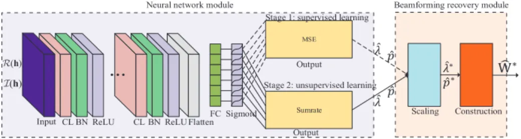
Fig. 4. BNN for the sum rate maximization problem.

B. Hybrid BNN Structure

The BNN for problem P3 is presented in Fig. 4. The major difference from the BNNs in

Figs. 2 and 3 is that the BNN in Fig. 4 has two stages of training. The first stage is responsible for pre-training using the supervised learning method with the loss function based on the MSE metric (24), while the second stage is responsible for enhanced training using the unsupervised learning method with the loss function whose metric is the objective function (25). Such a hybrid learning method of the supervised and unsupervised learning can significantly improve the learning performance and also accelerate convergence [29]. More specifically, the pre-training, as the approximation of WMMSE algorithm, starts with the random initialization of neural network parameters and the loss function (24). After the pre-training is finished, the neural network parameters are reserved and the loss function is replaced by (25), such that the second-stage training can achieve improved performance than the first-stage training.

Different from the BNNs in Figs. 2 and 3, the output layer in Fig. 4 generates 2K values

including the power allocation vectors pˆ and λˆ. Then the scaling layer scales the results of the

output layer qˆ and λˆ to meet the power constraint by the following method:

ˆ p∗ = Pmax ||pˆ||1 ˆ p and λˆ∗ = Pmax ||λˆ||1 ˆ λ. (26)

Finally, the construction layer constructs the downlink beamforming vectors according to (23): ˆ w∗_k=ppˆ∗_k (IN + PK k=1 ˆ λ∗ k σ2hkhHk ) −1_h k ||(IN +PK_k=1 ˆ λ∗_k σ2hkhHk)−1hk||2 ,∀k. (27)

˜

h

VII. SIMULATION RESULTS

To evaluate the performance of the proposed BNNs, we carry out numerical simulations to

compare the BNNs with several benchmark solutions (when available), including the optimal

beamforming,theZFbeamforming[58],theRZFbeamforming[59],andtheWMMSEalgorithm.

WeconsideradownlinktransmissionscenariowheretheBSisequippedwithN=6antennasand

itscoverageisadiscwitharadiusof500m.ThereareK=4single-antennausersandtheseusers

aredistributeduniformlywithinthecoverageoftheBS. Notethatnoneoftheseusersiscloserto

theBSthan100m.Thechannelofuserkismodelledashk=

√

dkh˜k∈CN×1where

k∼ CN (0, IN)is the small-scalefading[60] anddk= 128.1+ 37.6 log10(ω)[dB] denotesthe

pathloss between user k and the BS [61] with ω representing the distance in km. Here, shadow

fading isomitted for simplicity.The noise powerspectral density is−174 dBm/Hz and thetotal

system bandwidth is 20 MHz. For simplicity, we assume all the sub-streams have the same

importance and all the users have the same priority, i.e., ρk= 1, ∀k, and αk= 1, ∀k. Besides,

perfectCSIisassumedtobeavailableattheBS.

In our simulation, we prepare 20000 training samples and 5000 testing samples, respectively.

The validation split is set to 0.2 and the training data is randomly shuffled at each epoch. All

the BNNs have the same structure as shown in Table I. The fully-connected layer in the BNNs

for problems P1 and P2 has K neurons but that in the BNN for problem P3 has 2K neurons.

The Glorotnormal initializer[62] isused for weightinitialization andbiases areinitialized to 0.

Adam optimizer [63] is used with the MSE metric-based loss function. However, in the second

stage of the BNN for problem P3, the metric of the loss function becomes the sum rate. The

last activation layer is the sigmoid function so that the target output in the training and testing

samples should be normalized into (0,1] by dividing a factor. Also, the channel coefficients are

normalized bythe noise power beforebeing fed into the BNNsto avoid entering theinsensitive

areaofthesigmoidfunction. TheproposedBNNsolutionsareimplementedinPython3.6.5with

Tensorflow 1.2.1and Keras2.2.2 on a computerwith 1 Intel i7-7700U CPU Core and RAM of

32GB, andthe benchmarksare alsoimplementedin Python3.6.5 witha popularlibrary numpy.

Notethatunlessexplicitlymentionedotherwise, alltheneuralnetworkmodulesadoptthedefault

TABLE I

PARAMETERS OF THE NEURAL NETWORK MODULES.

Layer Parameter

Layer 1 (input) Input of size2×N K, batch of size 200, 100 epochs Layer 2 (convolutional) 8 kernels of3×3, zero padding 1, stride 1

Layer 3 (batch normalization) Momentum=0.99,= 0.001

Layer 4 (activation) ReLU

Layer 5 (convolutional) 8 kernels of3×3, zero padding 1, stride 1 Layer 7 (batch normalization) Momentum=0.99,= 0.001

Layer 6 (activation) ReLU Layer 8 (flatten)

Layer 9 (fully-connected) K or2Kneurons Layer 10 (activation) Sigmoid

Layer 11 output layer Adam optimizer, learning rate of 0.001, MSE metric

Normalized transmit power (dB)

0 5 10 15 20 25 30 SINR (dB) -10 -5 0 5 10 15 20 25 BNN Optimal ZF (a) Transmit power (dBm) 0 5 10 15 20 25 30 SINR (dB) -15 -10 -5 0 5 10 15 20 BNN Optimal ZF (b)

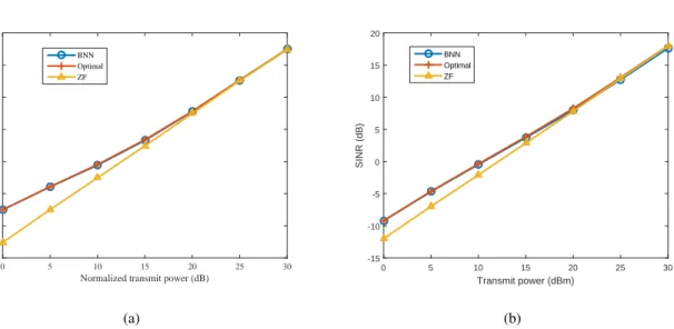
Fig. 5. The SINR performance averaged over 5000 samples in two different cases: (a) without large-scale fading and (b) with large-scale fading under{K= 4,N= 6}.

A. BNN for the SINR Balancing Problem

We first consider the BNN for the SINR balancing problem P1, which updates network

parameters in a supervised learning way. The iterative algorithm in [12, Table 1] is used to generate the training and testing samples. The ZF beamforming is achieved by allocating power to make all the users have the same SINR value under a total power constraint. Fig. 5 shows the SINR performance averaged over 5000 samples in two cases: one only considering the small-scale fading but the other considering both the small-small-scale fading and large-small-scale fading. In both

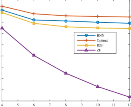
Transmit antenna number/ user number 4 5 6 7 8 9 10 11 12 SINR (dB) -4 -3 -2 -1 0 1 2 3 4 5 BNN Optimal RZF ZF

Fig. 6. Comparison of four different beamforming solutions, i.e., the optimal solution, the ZF beamforming, the RZF beamforming, and the BNN solution under {K = N, Pmax= 20dBm}.

Transmit antenna number

4 5 6 7 8 9 10 SINR (dB) 2 3 4 5 6 7 8 9 10 11 12 BNN Optimal ZF

Fig. 7. The SINR performance versus different transmit antenna numbers using the same trained BNN under{K= 4,N= 10,Pmax= 20dBm}.

cases, the SINR performance of the proposed BNN solution is very close to that of the optimal solution [12]. It is observed that there is an obvious gap between the optimal solution and the

ZF beamforming in the low normalized transmit-power (Pmax

σ2 ) regime of Fig. 5(a) as well as the

low transmit-power regime of Fig. 5(b). However, the gap decreases as the (normalized) transmit power increases.

To further compare the SINR performance of the optimal solution, the ZF beamforming,

the RZF beamforming whose regularization parameter is set as Pmax

K , and the BNN solution,

we evaluate the output SINR in Fig. 6 assuming that the number of users is the same as the

number of BS antennas, i.e., K = N, and they increase together. It is shown that the BNN

solution has some performance loss compared to the optimal solution due to the estimation error, but the BNN solution always achieves a better performance than the ZF beamforming and RZF beamforming. This fact indicates the application prospect of the BNN: the computational complexity and time of the BNN solution is similar to those of the ZF beamforming and RZF beamforming, but is much lower than that of the optimal solution because the optimal solution relies on an iterative process. Besides, we also find that the SINR performance of the four solutions decrease as the transmit antenna number (user number) increases and among the four solutions the ZF beamforming suffers most from the performance loss.

TABLE II

I/QTRANSFORMATION VERSUSP/MTRANSFORMATION.

K/N 4 6 8 10 12

I/Q transformation MSE 0.084 0.038 0.022 0.014 0.010 MAE 0.223 0.147 0.111 0.088 0.075 P/M transformation MSE 0.086 0.039 0.022 0.014 0.010 MAE 0.225 0.149 0.111 0.087 0.073

transformation, in terms of the MSE performance and MAE performance of the predicted

normalized power under the case with K =N and Pmax= 20 dBm. As shown in Table II, I/Q

transformation and P/M transformation have close performance.

In Fig. 7, we demonstrate the generality of the proposed BNN by fixing the user number as

K = 4 and the transmit power as Pmax = 20 dBm and show the SINR performance versus

different transmit antenna settings. We train only a single BNN with {K = 4, N = 10}, but

allow the number of transmit antennas to vary from 4 to 10 when using the trained BNN. Then the redundant entries at the inputs and outputs are filled with 0’s. It can be seen that these predicted results are very close to that of the optimal solution. This fact suggests the generality of the BNN, i.e., we can train a large BNN with more antennas which will also work for the cases with less antennas without re-training. This will be useful when some transmit antennas of the BS are malfunctioning or turned off.

B. BNN for the Power Minimization Problem

In this subsection, we consider the BNN for the power minimization problem P2, which also

updates network parameters in a supervised learning way. The iterative algorithm in [5] is used to generate the training and testing samples. The ZF beamforming for comparison is achieved by minimizing the power for each user with a QoS constraint since there is no inter-user interference. We first investigate the effect of the SINR constraints of users on the power consumption. For convenience of comparison, we assume the SINR constraints of all users are the same, i.e.

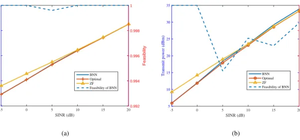
Γk = Γ,∀k. In Fig. 8, we compare the power performance of the optimal beamforming, the

ZF beamforming, and the beamforming obtained by the BNN. Note that both Figs. 8(a) and 8(b) have two Y-axes where the left Y-axis is used to measure the (normalized) transmit power averaged over the feasible sample set of the BNN solution and the right Y-axis is used to show

SINR (dB)

-5 0 5 10 15 20

Normalized transmit power (dB)

-10 0 10 20 30 Feasibility 0.992 0.994 0.996 0.998 1 BNN Optimal ZF Feasibility of BNN (a) SINR (dB) -5 0 5 10 15 20 Transmit power (dBm) 5 10 15 20 25 30 35 Feasibility 0.992 0.994 0.996 0.998 1 BNN Optimal ZF Feasibility of BNN (b)

Fig. 8. The power performance averaged over the feasible sample set of the BNN solution in two different cases: (a) without large-scale fading and (b) with large-scale fading under{K= 4,N= 6}.

the feasibility of the BNN. As mentioned in Section V, the BNN may fail to find a feasible

solution to problem P2 if the prediction error is unacceptable.

Figs. 8(a) and 8(b) present the (normalized) transmit power performance in the cases without and with consideration of the large-scale fading, respectively. In both cases, the (normalized) transmit power performance of the BNN solution is close to that of the optimal solution, and significantly outperforms the ZF beamforming in the low SINR-constraint regime which is higher than that of the optimal solution. We also find that, according to Fig. 8(b), the BNN solution performs slightly worse than the ZF solution when the SINR constraint is large, this is because the ZF solution becomes closer to the optimal solution as the SINR constraints increase, but the performance of the BNN solution is still close to that of the optimal solution. This fact suggests that when the SINR constraints are high, the ZF solution is a good choice instead of the BNN solution. Besides, we find that the feasibility of the BNN solution in both cases is more than 99.4%.

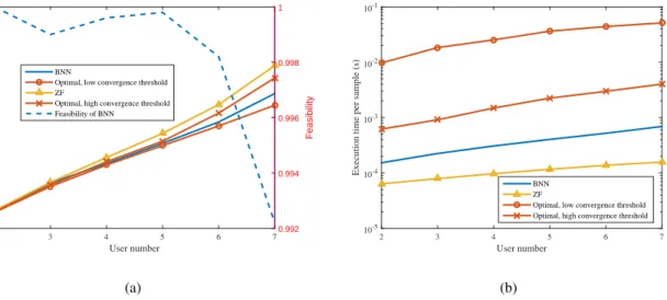
To further compare the BNN solution with the optimal solution and the ZF beamforming, we plot their power performance and execution time per sample in Figs. 9(a) and 9(b), re-spectively. Here, we consider two convergence strategies for the optimal iterative algorithm:

the high convergence threshold (ε1 = 10−2) which can be reached with less iterations and the

low convergence threshold (ε2 = 10−4) which requires more iterations for problem P2, i.e.,

|PK k=1||w (t−1) k || 2₋PK k=1||w (t) k || 2_| PK k=1||w (t−1) k ||2

User number 2 3 4 5 6 7 Transmit power (dBm) 10 15 20 25 30 Feasibility 0.992 0.994 0.996 0.998 1 BNN

Optimal, low convergence threshold ZF

Optimal, high convergence threshold Feasibility of BNN

(a)

User number

2 3 4 5 6 7

Execution time per sample (s)

10-5 10-4 10-3 10-2 10-1 BNN ZF

Optimal, low convergence threshold Optimal, high convergence threshold

(b)

Fig. 9. Comparison of three different beamforming solutions, i.e., the optimal solution, the BNN solution, and ZF beamforming: (a) power performance and (b) execution time per sample averaged over 5000 samples under{Γ = 5dB,N= 8}.

of users are fixed asN = 8 and Γ = 5 dB. It is observed from Fig. 9(a) that as the user number

K increases, the performance gap between the ZF beamforming and the optimal beamforming

with the low convergence threshold becomes large because more users share the array gain. The BNN solution, with the feasibility of up to 99%, shows a better performance than the ZF beamforming and the optimal iterative algorithm with the high convergence threshold. Fig. 9(b) demonstrates that compared to the optimal solution with the low convergence threshold, the BNN solution can reduce the execution time per sample by about two orders of magnitude, which is slightly longer than that of the ZF beamforming. This is because the BNN solution and the ZF beamforming are obtained without an iterative process, but the BNN needs to execute the neural network operations as well as the conversion process. We can reduce the iteration times using the high convergence threshold, but this leads to the power performance degradation. According to the results in Figs. 9(a) and 9(b), we can conclude that the BNN solution provides a good balance between the performance and computational complexity.

C. BNN for the Sum Rate Maximization Problem

In this subsection, we evaluate the performance of the BNN for the sum rate maximization

problemP3based on the proposed hybrid learning under the assumption thatK = 4andN = 4.

The ZF beamforming withpk = Pmax_K ,∀kand the RZF beamforming withpk =λk = Pmax_K ,∀kare

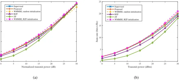
Normalized transmit power (dB)

0 5 10 15 20 25 30

Sum rate (bits/s/Hz)

0 5 10 15 20 25 30 Supervised Proposed

WMMSE, random initialization RZF ZF WMMSE, RZF initialization (a) Transmit power (dBm) 0 5 10 15 20 25 30

Sum rate (bits/s/Hz)

0 5 10 15 20 25 Supervised Proposed

WMMSE, random initialization RZF

ZF

WMMSE, RZF initialization

(b)

Fig. 10. The sum rate performance averaged over 5000 samples in two different cases: (a) without large-scale fading and (b) with large-scale fading under{K= 4,N= 4}.

relies on initialization [9, 10], two different initialization methods, the RZF initialization and the random initialization, are considered and the WMMSE algorithm with the RZF initialization is used to generate samples for the supervised learning in the first stage. First, Fig. 10 shows the sum rate performance averaged over 5000 samples in two different cases: the former case in Fig. 10(a) only considers small-scale fading and and the latter case in Fig. 10(b) considers both small-scale fading and large-scale fading. It is shown that the sum rate performance of all solutions increases as the (normalized) transmit power increases and different initialization methods of the WMMSE algorithm have a large performance gap. We observe that in both cases the proposed BNN solution based on the hybrid learning always achieves a performance close to that of the WMMSE algorithm with the RZF initialization, while the performance of the supervised learning-based BNN solution is less satisfactory. This is because the second stage of the hybrid learning method aims to maximize the sum rate and its performance is bounded

by the global optimal solution to problem P3. But the aim of the BNN solution based on the

supervised learning is to achieve as close to the WMMSE solution as possible and its performance is restricted by the WMMSE solution, which is verified in Figs. 10(a) and 10(b).

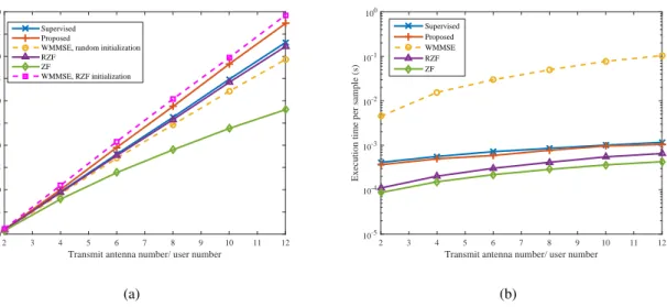
We further compare the sum rate performance and the computational complexity, in terms of the execution time per sample, of five beamforming solutions in Figs. 11(a) and 11(b), respectively. The iteration number of the WMMSE algorithm is limited to at most 10. We fix the

Transmit antenna number/ user number

2 3 4 5 6 7 8 9 10 11 12

Sum rate (bits/s/Hz)

10 15 20 25 30 35 40 45 50 55 60 Supervised Proposed

WMMSE, random initialization RZF

ZF

WMMSE, RZF initialization

(a)

Transmit antenna number/ user number

2 3 4 5 6 7 8 9 10 11 12

Execution time per sample (s)

10-5 10-4 10-3 10-2 10-1 100 Supervised Proposed WMMSE RZF ZF (b)

Fig.11. Comparisonoffivedifferentbeamformingsolutions,i.e.,theWMMSEsolution,BNNsolutionsbasedonthesupervised learningandtheproposedhybridlearning,respectively,theRZFbeamforming,andtheZFbeamforming:(a)sumrateperformance and(b)executiontimepersampleaveragedover5000samplesunder{K=N,Pmax=30dBm}.

as the user number, i.e., N = K. As the number of transmit antennas increases, the sum rate

performance of all five solutions increases simultaneously. The performance of the proposed

BNN solution based on the hybrid learning method is always close to that of the WMMSE

algorithm withthe RZF initialization, butis superior tothose of the otherfour solutionsand the

performance gap becomeslarger when the number of the transmitantenna increases. According

to Fig. 11(b), the execution time per sample of the BNN solutions based on the supervised

learning and hybrid learning methods is at the same level, which is slightly longer than that of

the ZF beamforming and the RZF beamforming, for the same reason of Fig. 9(b). As expected,

the WMMSE algorithm consumes the most time because of its iterative process. Similar to the

other proposed BNNs, it proves that the proposed BNN solution to the sum rate problem P3

provides a good balance between the performance and computational complexity.

VIII. CONCLUSIONS

In this paper, we proposed a DL-based framework for fast optimization of the beamforming

vectors in the MISO downlink and then devised three BNNs under this framework for the

SINR balancing problemunder a total power constraint, the power minimizationproblem under

individual QoS constraints, and the sum rate maximization problem under a total power

con-straint, respectively.The proposedBNNsare basedonthe CNNstructureand expertknowledge.

minimizationproblem becauseeffectivealgorithmsareavailablefor generatingtrainingsamples.

However, there is no practically useful algorithm to find the optimal solution to the nonconvex

sum rate maximization problem, therefore the corresponding BNN adoptes a hybrid learning

method which first pre-trains the neural network based on the supervised learning method,

and then updates the network parameters with the unsupervised learning method to further

improve learningperformance. Furthermore, in orderto reduce thecomplexity ofprediction, the

proposed BNNstakeadvantageof expertknowledgeto extractkey featuresinsteadof predicting

beamforming matrix directly. Simulation results demonstrated that the proposed BNN solutions

provided a good balance between the performance and computational complexity.

This work is an attempt to apply the DL technique to beamforming optimization. Actually,

a lot of extension works are worth further study. For example, it is unclear so far which input

format, I/Q transformationor P/Mtransformation, isbetter. In addition, thejoint optimizationof

user selection and beamforming design for the power minimization problem is interesting and

it deserves more investigation. Besides, user mobility, machine-type communications, imperfect

CSI, and multi-cell scenarios are also interesting extensions for future works.

REFERENCES

[1] W. Xia, G. Zheng, Y. Zhu, J. Zhang, J. Wang, and A. Petropulu, “Deep learning based beamforming neural networks in downlink MISO systems,” inProc. IEEE Int. Conf. Commun. (ICC) Workshop, Shanghai, China, May 2019, pp. 1–5. [2] E. Bj¨ornson, M. Bengtsson, and B. Ottersten, “Optimal multiuser transmit beamforming: A difficult problem with a simple

solution structure,”IEEE Signal Process. Mag., vol. 31, no. 4, pp. 142–148, Jul. 2014.

[3] H. Boche and M. Schubert, “A general duality theory for uplink and downlink beamforming,” inProc. IEEE Conf. Veh. Technol. Conf. (VTC), vol. 1, Vancouver, Canada, Sep. 2002, pp. 87–91.

[4] D. Gerlach and A. Paulraj, “Base station transmitting antenna arrays for multipath environments,”Signal Process., vol. 54, no. 1, pp. 59–73, Oct. 1996.

[5] Q. Shi, M. Razaviyayn, M. Hong, and Z. Luo, “SINR constrained beamforming for a MIMO multi-user downlink system: Algorithms and convergence analysis,”IEEE Trans. Signal Process., vol. 64, no. 11, pp. 2920–2933, Jun. 2016.

[6] F. Rashid-Farrokhi, K. R. Liu, and L. Tassiulas, “Transmit beamforming and power control for cellular wireless systems,”

IEEE J. Sel. Areas Commun., vol. 16, no. 8, pp. 1437–1450, Oct. 1998.

[7] A. B. Gershman, N. D. Sidiropoulos, S. Shahbazpanahi, M. Bengtsson, and B. Ottersten, “Convex optimization-based beamforming,”IEEE Signal Process. Mag., vol. 27, no. 3, pp. 62–75, May 2010.

[8] A. Wiesel, Y. C. Eldar, and S. Shamai, “Linear precoding via conic optimization for fixed MIMO receivers,”IEEE Trans. Signal Process., vol. 54, no. 1, pp. 161–176, Jan. 2006.

[9] Q. Shi, M. Razaviyayn, Z. Luo, and C. He, “An iteratively weighted MMSE approach to distributed sum-utility maximization for a MIMO interfering broadcast channel,”IEEE Trans. Signal Process., vol. 59, no. 9, pp. 4331–4340, Sep. 2011.