DP-F
AIR: A Simple Model for Understanding Optimal Multiprocessor Scheduling
Greg Levin
†, Shelby Funk
‡, Caitlin Sadowski
†, Ian Pye
†, Scott Brandt
††Computer Science Department ‡Department of Computer Science
University of California, Santa Cruz University of Georgia, Athens, GA
{glevin, supertri, ipye, sbrandt}@soe.ucsc.edu [email protected]
Abstract
We consider the problem of optimal real-time schedul-ing of periodic and sporadic tasks for identical multipro-cessors. A number of recent papers have used the notions offluid schedulinganddeadline partitioningto guarantee optimality and improve performance. In this paper, we develop a unifying theory with the DP-FAIR scheduling policy and examine how it overcomes problems faced by greedy scheduling algorithms. We then present a simple DP-FAIRscheduling algorithm,DP-WRAP, which serves as a least common ancestor to many recent algorithms. We also show how to extendDP-FAIRto the scheduling of spo-radic tasks with arbitrary deadlines.
1.
Introduction
Multiprocessor systems are becoming commonplace as more computers, even desktops, have multiple cores. Many implications of using a multiprocessor system, including scheduling issues, are still not well understood. Multipro-cessor scheduling is particularly difficult in the presence of hard real-time constraints. Real-time scheduling algo-rithms that are known to perform very well on uniprocessor systems, such as Earliest Deadline First (EDF) [21], do not perform as well on multiprocessors.
Broadly, there are two types of multiprocessor schedul-ing algorithms: globalandpartitioned. Global algorithms use a single scheduler for all processors and allow tasks to migrate between processors. Partitioned algorithms start by partitioning tasks among processors; scheduling is then handled by simpler uniprocessor algorithms, and no migra-tion is allowed. Partimigra-tioned approaches are easy to imple-ment, as they reduce multiprocessor scheduling to unipro-cessor scheduling. However, they are not optimal, in the sense that they can fail to schedule theoretically feasible task sets1.
1In fact, examples may be constructed where partitioned schedulers fail to successfully schedule tasks sets that only require(50 +)%of processor capacity [7, 22].
In 1996, Baruah et al. [5] introduced the PFAIR algo-rithm, the first optimal multiprocessor scheduler for peri-odic tasks. By migrating tasks between processors,PFAIR can successfully schedule any task set whose utilization does not exceed processor capacity. More recently, a num-ber of papers have exploited deadline partitioning (sub-dividing time into slices where all tasks have the same deadline) to achieve optimality while greatly reducing the number of required context switches and process migra-tions [3, 9, 26]. These and other algorithms, while superfi-cially different, have achieved optimality by expanding on the core idea of tracking thefluid schedule, or average rate curve. A better understanding of their shared traits will aid in the ability to understand, compare, and contrast these al-gorithms, to consolidate their insights, and to point towards new avenues of study.
The contributions of this papers are:
• We explore the difficulties of optimal multiprocessor scheduling and the failure of greedy algorithms.
• We give a simple set of guidelines, called DP-FAIR, for designing optimal schedulers for periodic task sets.
• We describe the DP-FAIRscheduling algorithm DP-WRAP(similar to EKG [3] and BF [26]), the simplest optimal scheduler to date, with reasonably good mi-gration bounds and limited computational overhead.
• We demonstrate the flexibility of the DP-FAIR guide-lines and the DP-WRAPalgorithm by extending them to handle sporadic task sets with arbitrary deadlines. The remainder of this paper is organized as follows. Section 2 formalizes the problem under consideration and provides relevant definitions. Section 3 examines why greedy scheduling algorithms (like EDF) tend to fail in a multiprocessor environment. Section 4 presents the DP-FAIRscheduling principles and proves their correctness; it also presents the simple DP-WRAPscheduling algorithm. Section 5 extends the DP-FAIRconditions to handle spo-radic tasks with arbitrary deadlines. Finally, Section 6 gives a brief survey of recent schedulers in the context of DP-FAIR.
m number of processors
n number of tasks
τ set of tasks{T1, . . . , Tn}
Ti ithtask
pi period (minimum interarrival time) ofTi
ei workload of each job ofTi
Di time between arrival and deadline ofTi
ai,h arrival time ofhthjob ofTi
δi ei/min{pi, Di} (density ofTi)
∆(τ) P
iδi (total density ofτ)
S(τ) m−∆(τ) (total slack ofτ)
σj jthtime slice, time interval =[tj−1, tj)
tj jthsystem deadline (end time ofσj)
Lj tj−tj−1 (length ofσj)
li,t local execution remaining forTiatt
ri,t li,t/(tj−t) (local utilization ofTiatt) Lt total local execution att
Rt total local utilization att
ci,t local capacity remaining forTiatt
αi,j(t) timeTihas been active inσjas oft
fi,j(t) timeTihas freed slack inσjas oft
wi,j(t) work executed byTiinσjas oft
Fj(t) Piδifi,j(t) (total slack freed inσjas oft)
Ij(t) total idle time inσjas oft
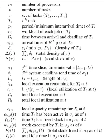
Figure 1.Summary of Notation
The first group of symbols defines a task set, the second group is used in Section 4, and the third in Section 5.
2.
Background
This paper considers the scheduling of n periodic or sporadic tasks on a system ofmidentical processors. With-out loss of generality, we assume the speed of each proces-sor is 1, i.e., each procesproces-sor performs one unit of work per unit of time. Each task will invoke a series of jobs, and each job requires a certain amount of work be performed before its deadline. Given a collection of periodic or spo-radic tasks, the basic problem is to find ascheduleto spec-ify which task (if any) runs on each processor at any given instant, with the restriction that no task can run on mul-tiple processors at the same time. We allow tasks to be preempted or to migrate between processors at any time.
A taskTi = (pi, ei, Di)is a process that invokes a
se-quence of jobs{Ti,h}h≥1. Each job Ti,h arrives at time
ai,h, and has an execution requirementeiand a deadline at
ai,h+Di. ThusTi,hmust be allowed to execute foreitime
units during the interval[ai,h, ai,h+Di). The minimum
time between the arrivals of the jobs ofTiispi. IfDi=pi,
we refer to this as animplicit deadlineand, dropping the implicitDi, use the abbreviated notationTi= (pi, ei);
oth-erwise, we say the task has anarbitrary deadline. IfTi is
Figure 2.Simple Scheduling Problem
Three tasks, each with a rate of2/3, can run successfully on two processors with migration.
a periodic task, then it invokes its first job at timet = 0 and all its remaining jobs are invoked exactlypitime units
apart, i.e.,ai,h = (h−1)pi for allh. IfTi is a sporadic
task, then it invokes its first job at any timet ≥0and the remaining jobs are invoked no less thanpitime units apart,
i.e.,ai,1≥0, andai,h≥ai,h−1+pifor allh >1. We let
τ ={T1, T2, . . . , Tn}denote a set ofnperiodic or sporadic
tasks.
One important parameter used to describe a taskTi is
itsutilizationui = ei/pi. For periodic tasks, the
utiliza-tion measures the proporutiliza-tion of time a task executes on average. For sporadic tasks, the utilization measures the “worst-case average”, i.e., the average proportion of re-quired computing time assuming a worst case sequence of arrivals (ai,j =ai,j−1+pi). The total utilization of task set
τ, denotedU(τ), is the sum of the individual utilizations:
U(τ) =
n X
i=1
ui .
When deadlines are not equal to periods, we instead use the task’sdensity,δi =ei/min{pi, Di}, and we let∆(τ)
denote the total density of the task set τ. Notice that if
Di = pi thenui = δi. For the remainder of the paper,
we will useδand∆for consistency, even when discussing utilization for tasks with implicit deadlines.
Avalidschedule is one where all jobs meet their dead-lines. We say that a set of tasks isfeasible if some valid schedule exists, and a scheduling algorithm isoptimalif it can successfully schedule any feasible task set. A simple example depicted in Figure 2 demonstrates a set of 3 tasks that can be successfully scheduled on two processors only when one of them divides its time between both CPUs.
Not all valid schedules are equally good. In order to re-duce overhead, scheduling algorithms must have short ex-ecution times and also try to minimize other costs, such as those associated with context switches and migrations. Al-though highly system-dependent, task migrations generally take longer than context switches, sometimes prohibitively longer. Because global scheduling algorithms migrate tasks and also tend to be complex (and, therefore, have long
run times), partitioned schemes are preferred in practice. Newer multiprocessor architectures, such as multicore pro-cessors, have significantly reduced the migration overhead. The preference for partitioned scheduling may no longer be necessary on these types of multiprocessors.
If we assume preemptions and migrations can occur in-stantly, then in theory it does not matterwhichprocessor is hosting a given task, only which tasks are running at a given time. This assumption can lead to clearer schedul-ing descriptions (e.g., Figures 2 & 4). In fact, some recent algorithms give no explicit prescription for how to assign tasks to processors [9, 13].
For now, we will focus on periodic task sets with im-plicit deadlines, and save the more general cases for Sec-tion 5. We will assume no scheduling overhead2, so that we should have enough CPU time to complete all jobs (i.e., the task set is feasible) provided:
(i) Total task workload doesn’t exceed total CPU capacity (∆(τ)≤m).
(ii) No task’s workload exceeds its period or deadline (δi≤1 ∀i).
(iii) Process migration is allowed.
Given unlimited context switching and migration, it is not hard to see that any task set satisfying these conditions will be feasible. This fact is just an extension of the unipro-cessor case presented by Liu and Layland [21]. Imagine that we can reschedule our jobs after eachof time. As
→0, we can turn each taskTion or off sufficiently often
so that it appears to be constantly running on only a fraction
δiof a processor. In the limit, each job executes at exactly
its necessary rate and, when all rates sum to no more than
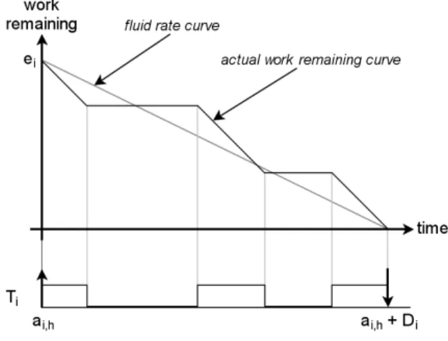
m, all jobs finish on time. Srinivasan et al. [25] refer to this as afluidscheduling model. Figure 3 shows the fluid and actual scheduling of a task.
Determining the feasibility of a periodic task set with implicit deadlines is easy; much more challenging is ac-tually finding a valid schedule that minimizes context switches and migrations. This has been the goal of recent papers in this problem domain, and is our primary interest. To motivate our approach, we explore the shortcomings of greedy schedulers.
3.
Greedy Schedulers
An attractive (and common [7]) first approach to scheduling is to try to find a simple greedy solution. Greedy algorithms are straightforward to explain, prove and im-plement. They often attempt to encapsulate the criticality 2Alternatively, we can assume the overhead costs are included in the tasks’ execution requirements. This is a valid assumption if the worst-case number of preemptions and migrations can be determined in advance, which is often the case. However, this implementation could lead to very pessimistic worst case execution times.
Figure 3.Fluid versus Practical Schedules
(likeliness of a missed deadline) of a job into a single quan-tity and then use that to greedily schedule jobs.
Two common greedy algorithms for uniprocessor scheduling are Earliest Deadline First (EDF) [21] and Least Laxity First (LLF) [24]. As their names imply, these algo-rithms give execution priority to the job with the earliest deadline or least laxity, respectively. Thelaxityof a job is the difference between its time and work remaining until its deadline. Although LLF has a higher scheduling over-head, both algorithms are optimal on a single processor; unfortunately, neither is optimal on a multiprocessor ( [18], Figure 4a).
The LLF scheduler is based partially on the observation that a schedule has become infeasible if any job ever has negative laxity (more work than time remaining). Clearly, any job whose laxity has reached zero must be immediately activated and run continuously until its deadline in order to complete its work on time. This observation leads us to our second consideration when designing a greedy algo-rithm. The “greedy” part tells uswhichtasks to schedule, but we must also specify whenthe algorithm will do the scheduling. That is, at what times should re-sorting and the application of the greedy preference occur? Three standard scheduling events are:
RELEASE: A task is at the beginning of its period; WORKCOMPLETE: A task has finished its work for its
current period, and must be turned off;
ZEROLAXITY: A task has no remaining laxity for its current period, and must be turned on.
Any simple greedy algorithm must specify its greedy sort key and which scheduling events it will observe. For example, when ZERO LAXITY events are added to EDF, the result is a hybrid scheduler known as EDZL [10]. While this provides an improvement over standard EDF for mul-tiprocessors, EDZL is still not optimal.
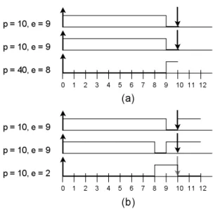
Figure 4.Greedy Counter-example
Task set which confounds known greedy schedulers using common events. (a) shows an incorrect greedy scheduling, while (b) shows a feasible proportional scheduling.
3.1.
Why Greedy Schedulers Fail
To improve upon greedy schedulers, it is necessary to understand why they fail. Consider the feasible task set
{T1= (10,9), T2= (10,9), T3= (40,8)}
shown in Figure 4(a); LLF cannot successfully schedule this job set on two processors. T1andT2each have laxity
of 1, and so are prioritized and run to completion whileT3’s
laxity drops from 32 to 23. WhenT1andT2finish att= 9,
T3is the only task with work remaining. One processor is
idle untilT1andT2are re-released att= 10.
In fact, it seems implausible thatanygreedy scheduler would choose to activateT3beforet = 9. Even att = 8,
T1 andT2 have earlier deadlines, lower laxity, higher
to-tal and remaining utilizations, etc. It is difficult to envision an intelligent criterion which would preferT3. And yet, if
T3 is not activated byt = 8, a deadline will eventually be
missed3. The following theorem generalizes this observa-tion.
Theorem 1 When the total utilization of a periodic task set is equal to the number of processors, then no feasible schedule can allow any processor to remain idle for any length of time.
Proof. Given tasksT1, . . . , Tnonmprocessors where the
rates sum tom. In a feasible schedule, taskTi, at the end of
3Betweent= 0andt= 40,(2×4×9) + 8 = 80units of work must be done, though the two processors can only accomplish 79 if one is idle betweent= 9and 10.
hperiods, must have done work equal tohei=h(piδi) =
(hpi)δi = ah+1δi, whereah+1 is the ending time of the
hth period. Let t0 be the first positive time at which all
tasks reach a deadline simultaneously (i.e., the least com-mon multiple of their periods). Then the total work done by all tasks by timet0must beP
it 0δ
i=t0Piδi=t0m. This
much work can be accomplished by timet0only if all pro-cessors are running continuously until this time. Any idle time implies less thant0m total work is done, and some
deadline will be missed.
Clearly something critical is happening at timet= 8in our example, but no obvious scheduling event occurs here, and no reasonable greedy sort would respond correctly. Only by consideringT1andT2as a setcan we see that they
leave two units of idle time to be filled by timet= 10, and that one job cannot fill this time on two processors simulta-neously. When greedy algorithms fail, it is usually for lack of some global knowledge. In our case, such knowledge is implicitly provided by a single over-constraint.
4.
Deadline Partitioning and DP-F
AIRTo date, the only known solutions to the “global knowl-edge” problem are variations on proportional fairness. By over-constraining our scheduling requirements, propor-tional fairness forces tasks to march in step with their fluid rate curves more precisely than is theoretically necessary. Suppose we modify our previous example to
{T1= (10,9), T2= (10,9), T3= (10,2)} .
All we have done is to impose the additional requirement that taskT3complete a proportional share of its work every
time the other tasks hit their deadlines. Suddenly we have a ZEROLAXITYevent at time 8.T3will then be switched on;
T1andT2will each run for one of the remaining two time
units on the other processor, and a feasible schedule results (see Figure 4b). In this example, where the third period was a multiple of the first two, it is easy to reformulate the problem in this way. When we have numerous jobs with disparate periods, the question of when to force jobs to hit their proportional rate quotas is not immediately obvious.
The first solution to this problem was thePFAIR schedul-ing scheme [5]. PFAIRcreates a scheduling event and re-computes the set of running tasks at every multiple of a discrete time quantum. The notion of proportional fairness used is very strict, requiring the actual work completed by a task to be within 1 unit of its fluid rate curve at each time quantum. The result of this policy is a large number of scheduling calculations and context switches, with corre-spondingly high overhead. Intuitively, it seems unneces-sary to adhere so closely to the fluid schedule: performance could be improved by a more judicious choice of schedul-ing events.
4.1.
DP-F
AIRConditions for Periodic Tasks
To motivate our next step, recall the following result by Hong and Leung [15].
Theorem 2 No optimal on-line scheduler can exist for a set of jobswith two or more distinct deadlineson anym -processor system, wherem >1. ♦ Note that Theorem 2 does not apply when all dead-lines are equal. In fact, Hong and Leung also present the RESCHEDULEalgorithm, which they prove is optimal when all jobs have the same deadline, even when some ar-rival times are unknown. Their RESCHEDULEalgorithm is similar in design to our own DP-WRAPalgorithm in Sec-tion 4.2. Let us first consider the benefit offorcingall jobs to have the same deadline.
Deadline partitioning(DP) is the technique of partition-ing time intoslices, demarcated by all the deadlines of all tasks in the system. Within each slice, all jobs are allo-cated a workload for the time slice and these workloads share the same deadline. While a number of recent algo-rithms [3, 9, 26] have used deadline partitioning, there has not previously been a unifying theory for why this tech-nique is so effective. With the DP-FAIR conditions pre-sented below, we provide such a theory.
There are two aspects to deadline partitioning: allocat-ing the workloads for all tasks for each time slice, and schedulingwithin a time slice. We say that an algorithm using this approach is DP-CORRECT if (i) the time slice scheduler will execute all jobs’ allocated workload by the end of the time slice whenever it is possible to do so, and (ii) jobs are allocated workloads for each slice so that it is possible to complete this work within the slice, and com-pletion of these workloads causes all tasks’ actual deadlines to be met. In other words, any DP-CORRECTscheduler is optimal.
Before we proceed, we will require some additional no-tation. We lett0= 0andt1, t2, . . .denote the distinct
dead-lines of all tasks inτ, wheretj < tj+1for allj ≥0. Then
thejthtime slice, denotedσ
j, is[tj−1, tj), and has length
Lj=tj−tj−1. Unless otherwise noted, we only consider
one time sliceσjat a time. As general conventions, when
timetis a parameter, we will subscript (e.g.,Xt) to refer
to “remainingX”, and parenthesize (e.g.,X(t)) to refer to “X so far”. Subscripthwill index thehthjob in a task,i
will represent taskTi, andjis for time sliceσj.
We analyze schedules by considering execution during
σj, drawing heavily on notation from the LLREF
schedul-ing algorithm [9]. Thelocal execution remainingof a task
Tiat timet, denoted`i,t, is the amount of time thatTimust
execute before the next time slice boundary, i.e., between timestandtj. A task’slocal utilizationri,t=`i,t/(tj−t)
is the proportion of time betweent and tj that Ti must
spend executing. We let Lt and Rt denote a task set’s
summed local remaining execution and utilization, respec-tively, at timet.
The scheduling process is most easily understood when the task set has full utilization, i.e., ∆(τ) = m. Since we do not generally expect full utilization, one or more dummy tasks may be introduced to make up the differ-ence. With this intent, we define theslackof a task set to be
S(τ) =m−∆(τ). Consider a time slice of length 10 on 2 processors, and a task set with∆(τ) = 1.5. The system has the capacity to do 20 units of work, but with only 15 units of work to be done, 5 units of idle time must appear somewhere within the slice. While common sense might dictate that an algorithm should always be doing work if there is work to be done, and that the idle time should there-fore come at the end of the slice, this is an unnecessary over-constraint on algorithm design. By viewing slack as a dummy job and idle time as a necessary activity, we pro-vide maximum freedom in scheduling the time slice.
Note that our description of idle time as a capacity-consuming resource, and our attempts to provide maxi-mum flexibility in scheduling it, are not just for conve-nience. While our model treats it as dead processor time, that “dead time” can actually be employed for a num-ber of purposes, including load balancing [4], improving performance [3, 19], creating a work-conserving scheduler [12, 13], or running non-real-time tasks in a hybrid sys-tem [20].
We now propose a minimally restrictive set of schedul-ing rules, DP-FAIR, which ensure that an algorithm is DP-CORRECT and provide substantial latitude for algorithm design. DP-FAIRAllocation for periodic task sets with im-plicit deadlines is quite simple: ensure that all tasks hit their fluid rate curves at the end of each slice by assigning each task a workload proportional to its utilization; that is, task
Tiis assigned workload`i,tj−1 =δi×Ljfor time sliceσj.
With these allocations in mind, we are ready to formulate our DP-FAIRScheduling conditions.Fj(t)in RULE3 is a
freed slackterm that will be used in Section 5, but for now is just zero.
Definition 1 (DP-FAIR Scheduling for time slices) A slice-scheduling algorithm isDP-FAIRif it schedules jobs within a time sliceσjaccording to the following rules:
RULE1:Always run a job with zero local laxity; RULE2:Never run a job with no remaining local work; RULE3:Do not voluntarily allow more than
(S(τ)×Lj) +Fj(t)units of idle time to occur inσj
before timet. ♦
We now prove that any DP-FAIRscheduler is optimal via a pair of Lemmas.
Lemma 3 If tasksτ are scheduled within a time slice ac-cording toDP-FAIR, andRt≤mat all timest∈σj, then
all tasks inτ will meet their local deadlines at the end of the slice.
Proof. A task can only miss its (local) deadline if it achieves negative (local) laxity. However, by RULE1, any job that hits zero laxity will be run to completion on some processor. The only way this scheme can fail to finish all jobs’ local workloads on time is if more thanmjobs simul-taneously have zero laxity, so that one of them cannot be run. Since a zero laxity job hasri,t = 1, we would have
Rt≥m+ 1, contradicting our assumption. Lemma 4 If a set τ of periodic tasks with implicit dead-lines is scheduled inσjusing anyDP-FAIRalgorithm, then
Rt≤mwill hold at all timest∈σj.
Proof.Let us introduce the dummy jobTn+1representing
idle time, and give it utilizationS(τ). Note thatTn+1’s
uti-lization can be larger than 1, since this one “job” is allowed to run on multiple processors at once. (To stay closer to our task model, we could introduceS(τ)/jobs, each with utilization, and let→0. For this proof, this is an unnec-essary complication.) We let`n+1,tbe the portion of the
totalS(τ)×Ljidle time inσjnot yet used up as of timet,
and let Lt = n X i=1 `i,t and L0t = n+1 X i=1 `i,t
be the work remaining at time t in our original and ex-tended task sets, respectively. Now, themprocessors are consuming the workload fromT1, . . . , Tn+1 at a rate of
m per time unit, so of the mLj units of work and idle
time that needed to be consumed at the beginning ofσj,
m(tj−tj−1)−m(t−tj−1) =m(tj−t)remain at timet, i.e.,L0 t=m(tj−t). Then Rt = n X i=1 `i,t tj−t ≤ 1 tj−t n+1 X i=1 `i,t = L0 t tj−t = m , as desired.
Theorem 5 Any DP-FAIRscheduling algorithm for peri-odic task sets with implicit deadlines is optimal.
Proof. Lemmas 3 and 4 show that all tasks will meet all local deadlines at the end of time slices by following DP-FAIR’s rules; that is, each job’s work completed will match its fluid rate curve ateverysystem deadline, including its own. Since anyTi’s fluid rate curve is zero at its own
dead-lines, it follows thatTiwill meet its deadlines. This holds
for all jobs from all tasks, so any DP-FAIR algorithm is
optimal.
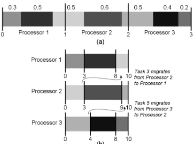
Figure 5.The DP-WRAPAlgorithm
(a)Seven tasks with utilizations shown above. These are lined up in arbitrary order, then split at length 1 intervals.
(b)Each processor runs its task set over a length 10 time slice. Jobs sliced in (a) are seen migrating in (b).
RULES1-3 of Definition 1 are about as simple a set of criteria as one could hope for. In essence,
“If a job needs to be started now in order to finish on time, then start it. If a job finishes, then stop it. Don’t allow idle time in excess of the task set’s slack.”
These three rules, although an overconstraint when ap-plied at every slice boundary, are obviously necessary to keep tasks hitting their fluid rate curves. Yet, when we re-quire proportional workloads be completed at all system deadlines (DP-FAIR Allocation), they are also sufficient. As these rules are so simple, they leave plenty of room to design scheduling algorithms that attempt to reduce the number of context switches and task migrations or address variants of the basic problem model.
4.2.
The DP-W
RAPAlgorithm for Periodic Tasks
We now present our DP-WRAPalgorithm. DP-WRAP is a simplification of EKG [3], and is perhaps the simplest possible DP-FAIRscheduler. The algorithm may be visu-alized as follows. To schedule jobs inσj, make a “block”
of length δi for each Ti, and line these blocks up along
a number line (in any order), starting at zero. Their total length will be no more thanm. Split this stack of blocks into length 1 chunks at1,2, . . . , m−1, and assign each chunk to its own processor. Each length 1 chunk of tasks represents the scheduling of tasks on the respective pro-cessor; tasks which are sliced in two migrate between their two processors (this task-to-processor scheme is essentially McNaughton’s wrap around algorithm [23]). See Figure 5 for an illustration with 7 tasks and 3 processors. To find the actual timing points of context switches (at local WORK
COMPLETEevents) within anyσj, multiply each length 1
segment byLj.
It is immediately clear from this description that all three DP-FAIRscheduling rules are satisfied. Tasks which mi-grate are run at the beginning of the slice on one proces-sor, and at the end on the other. So long as such a task has utilization no more than 1 (which is required forany feasible schedule), its running times on the two processors will not overlap. We now have the straightforward DP-WRAPscheduling algorithm: compute the context switch times indicated in the diagram (partial sums of task uti-lizations), reduce modulo 1 for each processor, and mul-tiply times byLj. Except for this last multiplication, all
calculations can be done once as a preprocessing step, so long as the task set is static. Note that there isno compu-tational overhead at secondary events: here, a “schedul-ing event” (which in many algorithms requires iterat“schedul-ing through all jobs, performing various calculations, or even sorting them) is merely following a predetermined instruc-tion to replace one task with another on one processor; no “decisions” are made.
Notice that, in general, there will bem−1tasks which are required to migrate. Further, if we repeat a predeter-mined ordering for each time slice, each of thesem−1 tasks will migratetwiceper window: once in the middle, and again at the end, when it moves back to its starting pro-cessor. We can cut this number of migrations in half simply by reversing (mirroring[3]) the ordering of tasks on each processor in odd-numbered slices. Looking at the example in Figure 5, task 3 runs for the first 0.3 of the window on processor 2, then for the last 0.2 on processor 1. If we re-verse the ordering within each processor for the next slice, then task 3 willstarton processor 1 (for 0.2) and thenfinish on processor 2 (for 0.3).
Theorem 6 The DP-WRAP scheduling algorithm with mirroring in odd slices will produce at mostn−1context switches andm−1migrations per slice.
Proof. With mirroring, context switches and migrations only occur in the middle of a slice, never at the end. In the worst case, every job except the first causes a context switch when it is started, resulting isn−1context switches per slice. There arem−1tasks which migrate once each
per slice.
Various heuristics could be added to improve DP-WRAP’s performance in terms of context switches and mi-grations (e.g., EKG). Instead, we present DP-WRAPin its simplest form to demonstrate how the DP-FAIR schedul-ing rules can lead to a minimal optimal algorithm, which is both easy to describe and implement, and which requires little computational overhead.
5.
DP-F
AIRConditions for Sporadic Tasks
and (Un)constrained Deadlines
Due to their simplicity, the DP-FAIR scheduling rules may be extended to various generalizations of the schedul-ing problem without excess complications. In this section, we will see how to expand DP-FAIRto handle tasks with sporadic job arrivals. We will also consider constrained deadlines, whereDi ≤piand, consequently,δi =ei/Di;
the case ofarbitrarydeadlines (additionally allowingDi>
pi) is addressed in Section 5.2. We will give more detailed
rules for how to allocate workloads within a time slice in these cases; the rules for scheduling in a time slice remain the same, except that we now use theFj(t)term in RULE3.
We maintain the (sufficient but no longer necessary) re-quirements that ∆(τ) ≤ m and δi ≤ 1 ∀i. Because
there exist feasible task sets with sporadic arrivals where these conditions are violated4, and our extended DP-FAIR
rules do not handle these cases, DP-FAIR algorithms are no longer optimal. In fact, it has recently been shown that there can be no optimal algorithm for sporadic task sets [11]. Thus we will limit ourselves to showing that DP-FAIRalgorithms are optimal on task sets with∆(τ)≤m
andδi≤1∀i.
In the domain of sporadic tasks and constrained dead-lines, a task may not use all the capacity reserved for it. Sinceδi =ei/DiwhenDi < pi, the time between
dead-line and next period represents unused capacity. The same is true for the late time between earliest possible and ac-tual arrivals for a sporadic task. During this time (i.e., be-tweenai,h−1+Diandai,h), we say that a task isfreeing
slack(orinactive); a task isactivebetween timesai,hand
ai,h+Di (even if it has no work remaining). Thus, for
each task, time is partitioned into slack freeing and active periods. Because∆(τ)≤m,Ti“owns” a portionδiof the
system’s total capacitym, even during times when the task is inactive. For this reason, we still attach a task’s freed slack to it for accounting purposes, even though this slack goes into the system’s general pool of idle processor time.
Similarly to how`i,trepresents local execution time
re-maining, we will letci,trepresentlocal capacityremaining
for task Ti at time t. Local execution is only consumed
(at a rate of 1) when the task is executing; local capacity is consumed either by the task executing (at a rate of 1) or freeing slack (at a rate ofδi). We defineαi,j(t)andfi,j(t)
to be the amounts of time thatTihas been active or freeing
slack, respectively, during sliceσjas of timet. We usefi,j
andαi,jas shorthands forfi,j(tj)andαi,j(tj).
In time sliceσj,Tiwill be allotted a total ofδi×αi,j
local execution time (although this must be allocated
dy-4For example,T
1= (2,1,1)andT2= (2,1,2)onm= 1processor
namically as new jobs arrive), and fixed local capacity
ci,tj−1 = δi×Lj = δi(αi,j+fi,j)
Finally, we define thefreed slack inσjas of timetto be
Fj(t) = n X
i=1
(δi×fi,j(t)) .
We now present two rules for work allocation in our new problem domain.
Definition 2 (DP-FAIR Allocation for sporadic tasks and constrained deadlines)An algorithm hasDP-FAIR Alloca-tionif, for every time sliceσj, local execution is allocated
according to the following rules:
RULE4: Initialize`i,tj−1 to 0. At the beginning time
t0 of any active time segment for Ti in σj (either
t0 =tj−1orai,h) that ends at timet00= min{ai,h+
Di, tj}, increment`i,tbyδi(t00−t0).
RULE5:If a taskTiarrives and has a deadline within
the same time sliceσj, split the remainder ofσjinto
two secondary slicesσj1andσj2so thatTi’s deadline
coincides with the end ofσ1
j. Divide remaining local
execution (and capacity) of all jobs (as well as slack allotment forRULE3) in proportion to the lengths of
σ1
j andσj2. This rule may be invoked repeatedly /
re-cursively by multipleTiwithinσj. ♦
Since we requireDi ≤ pi, an active period forTi can
only end at a task deadline, not the end of a period. Since RULE 5 creates a new slice whenever a deadline appears within an existing slice, all deadlines form the end of some slice. Thus, once a job is active within some slice, it cannot become inactive before the end of that slice. Now, δi×
αi,jwork is required ofTiinσj, so`i,tis incremented by
δi×αi,jwheneverTibecomes active inσj(which will be
attj−1 if the task startsσj with work remaining). Since
ci,tj−1 =δi(αi,j+fi,j), we will haveci,t> `i,tso long as
Tiis freeing slack, andci,t=`i,tonceTibecomes active.
Lemma 3 from the previous section makes no assump-tion about deadlines or periodicity, and so is still valid in this extended problem domain. Thus, to prove the correct-ness of these new DP-FAIRconditions, it only remains to show thatRt≤mfor allt∈σj, and that RULE5 suffices
to meet deadlines introduced in the middle ofσj.
Lemma 7 ADP-FAIRalgorithm cannot cause more than (S(τ)×Lj) +Fj(t)units of idle time in sliceσjprior to
timet.
Proof. Since RULE3 prohibitsvoluntaryidle time in ex-cess of this amount and Fj(t) is a non-decreasing
func-tion, we only need to prove that mandatory idle time (when
we have fewer jobs with work remaining than processors) cannot force this limit to be broken. Let Ij(t) be the
amount of idle time as of timet during sliceσj. For the
sake of contradiction, lett0 be the first failure point inσj.
SinceIj andFj are continuous functions oft, this means
that Ij(t0) = (S(τ)×Lj) +Fj(t0) and Ij(t0 +) >
(S(τ)×Lj) +Fj(t0+)for all sufficiently small >0.
Since tasks can’t switch from active to inactive in the middle of a slice, if a task has no work to do at timet0, it is either because it has not yet become active, or because it has finished its entire workload for the current slice. We can therefore partitionτ into three sets at time t0: letA
be the set of active tasks with work remaining, B be the set of unarrived (slack freeing) tasks, and Cbe the set of tasks that have arrived and completed their allotted work for σj. For convenience, we will let ∆X =Pi∈Xδi for
X ∈ {A, B, C}.
Based on our definition of local capacity, any task Ti
should account for δiLj processor time duringσj with a
combination of work done and idle time from slack freed. At timet0, all freed slack has been consumed as idle time, so tasks inBhave used exactly their allotment of processor time so far. Ctasks, on the other hand, have already used allof their allotted time, having freed their slack (if any) and finished their workloads. That is, they have consumed ∆CLjprocessor time, and are∆C(tj−t0)aheadof their
fair share at timet0. Similarly, the static slack poolS(τ)Lj
is already consumed, and so isS(τ)(tj−t0)ahead of its
proportional allotment at timet0. This means that tasks in
Amust be collectively(∆C+S(τ))(tj−t0)unitsbehind
on their use of processor time. If they were keeping up, they would have∆A(tj −t0)work remaining, so as it is
they must have exactly
∆A(tj−t0) + (∆C+S(τ))(tj−t0) = (m−∆B)(tj−t0)
work remaining, since∆A+ ∆B+ ∆C+S(τ) =m.
Given our definition oft0, RULE3 tells us that we can-not choose to idle processors at timet0. If|A| ≥ m, then we can runmtasks at timet0. Ij(t)will not immediately
increase, contradicting our definition oft0. Thus, we must have|A|< m. By RULE1, we know that each job inA, if left to run on its own processor, will finish its work on time. ThusAcan’t have more than|A|(tj−t0)work remaining.
From above,
(m−∆B)(tj−t0)≤ |A|(tj−t0) ⇒ ∆B ≥m− |A| .
Tasks in B are freeing slack at a rate of ∆B at time t0;
the system is only adding idle time at a rate of m− |A|. ThenFj(t)is growing faster thanIj(t)at timet0, andIj(t)
cannot immediately exceedS(τ)Lj+Fj(t), again
contra-dicting our definition oft0. Since there can be no first point
Lemma 8 If a set τ of sporadic tasks with constrained deadlines is scheduled inσjusing anyDP-FAIRalgorithm,
thenRt≤mwill hold at all timest∈σj.
Proof.As of timet∈σj, the system has consumedm(t−
tj−1)capacity, either by executing jobs, or by idling. If it
has idled forIj(t)time units by timetthen Lemma 7 gives
Ij(t) ≤ S(τ)Lj +Fj(t). If we letwi,j(t) be the work
executed on taskTiduringσjas of timet, then we have
m(t−tj−1) = Ij(t) + n X i=1 wi,j(t) , (1) and
ci,t = ci,tj−1−wi,j(t)−δifi,j(t)
= δiLj−wi,j(t)−δifi,j(t) . (2)
Recalling thatri,t(tj−t) =`i,t≤ci,t,
Rt(tj−t) = n X i=1 `i,t ≤ n X i=1 ci,t = n X i=1 (δiLj−wi,j(t)−δifi,j(t)) by (2) = ∆(τ)Lj− n X i=1 wi,j(t)−Fj(t) ≤ (m−S(τ))Lj− n X i=1 wi,j(t) + (S(τ)Lj−Ij(t)) = mLj−(m(t−tj−1)) by (1) = m(tj−t)
and we see thatRt≤m, as desired.
Theorem 9 AnyDP-FAIRscheduling algorithm is optimal for sporadic task sets with constrained deadlines where ∆(τ)≤mandδi≤1∀i.
Proof. As in Theorem 5, all tasks finishing their local workloads at the end of time slices ensures that they hit their fluid rate curves at their deadlines, i.e., they don’t miss their deadlines. The only remaining questions are whether a task which arrives and has its deadline within a slice will meet this deadline, and whether RULE5 will interfere with other tasks completing their workloads.
If task Ti has an arrival at time t0 = ai,h in σj, then
m(t0−tj−1)work and idle time have been consumed thus
far in the slice, and the remaining capacity ofm(tj−t0)is
exactly enough to complete each task’s allotment ofδiLj
plus consume theS(τ)Lj static slack. If we create
sub-slicesσ1
j = [t0, t00)andσ2j = [t00, tj), wheret00=ai,h+Di,
and divide remaining work for each task and idle time be-tween these subslices proportionally to their lengths, then
each subslice will have been given a work/slack load ex-actly equal to its capacity. Lemmas 3 and 8 prove that, by following a DP-FAIR slice scheduling policy, these workloads will be successfully completed. Any other task
Ti0 6= Ti has its remaining work divided betweenσ1j and
σ2
j, and so it is finished by the end ofσj, as it requires.
As forTi, since it has been freeing slack prior tot0, it has
exactlyδi(tj−t0)capacity reserved for the remainder ofσj.
Ticlaims the proper proportionδi(t00−t0) =δiDi=eiof
this capacity for execution inσj1, and gets exactly enough work done to meet its deadline.
5.1.
Modifying DP-W
RAPModifying DP-WRAPto handle arrivals within a time slice is fairly straightforward. If a taskTigenerates a job at
timet0within time sliceσjandt0+Di≥tj, then we
allo-cate execution time`i,t0=δi(tj−t0), as per RULE4. This execution is wrapped onto the end of the existing schedule without otherwise impacting the schedule forσj.
Ift0+D
i < tj, then we need to split the remainder of
σjinto two subslicesσ1j andσ2j according to RULE5.Ti’s
workload is given entirely toσ1
j. The remaining workloads
of all other tasks are divided proportionally betweenσj1and
σ2
j. Each subslice is scheduled as described in Section 4.2.
5.2.
Arbitrary Deadlines
Let us now consider the problem where deadlines can be larger than periods via the following example.
Example Consider the periodic task set τ on m = 2 processors where T1 = (6,4) and T2 = T3 = T4 =
T5 = (3,1,6). Since∆(τ) = 4/6 + 4(1/3) = 2, and
4 + 4×2×1 = 12units of work must be done by time 6 in order to meet our time slice deadlines, the system can allow no idle time. However, if we runT2thenT3to
com-pletion on the first processor andT4thenT5on the second,
then at time 2, tasksT2, . . . , T5are out of work. Only at
this point is T1 forced to run by zero laxity. Until more
work arrives forT2, . . . , T5 at time 3, the other processor
sits idle, implying eventual failure by Theorem 1. ♦
Allowing deadlines longer than periods breaks the “global knowledge” granted by giving all tasks the same deadlines. Fortunately, the problem is easily solved. If we are given a task whereDi> pi, we simply impose an
arti-ficial deadline ofDi0 =pi. This doesn’t increase the task’s
densityδi, and if the artificial deadline is met, the real one
will certainly be also. However, these artificial deadlines might force unnecessary slice boundaries. In the absence of artificial deadlines, if a task were to finish its workload in some slice prior to its deadline, then that period of the task wouldn’t create any slice boundary. Increasing the number of time slices, in turn, incurs additional overhead from the added context switches and migrations.
5.3.
Some Simplifications
RULE5’s time slice splitting could be very complicated, particularly if it is done recursively for several tasks within a single time slice. We can avoid ever having to split time slices in this manner by ensuring time slices are never longer than the minimum deadline. Like our solution for arbitrary deadlines, this simplifies scheduling but increases context switches and migrations.
We could also simplify RULE3 by replacing it with suf-ficiently strong heuristics. A simple one is “Never allow a processor to idle if there are tasks waiting to execute.” A somewhat less restrictive rule is “At all timest, at least
dRtetasks are executing jobs.” These rules would be easier
to implement in practice, and also satisfy RULE3.
6.
Related Work
We now examine some recent algorithms in the con-text of DP-FAIR. Unless otherwise noted, the following algorithms only address periodic task sets with implicit deadlines. PFAIR [5] was the first optimal multiprocessor scheduler. It uses a very strict notion of proportional fair-ness to target fluid rate curves at every multiple of a dis-crete time quantum, and incurs a large overhead in context switches and migrations. The 2003 BF Algorithm [26] ap-pears to be the first use of deadline partitioning for real-time scheduling. BF modifiesPFAIR, and is still quantum-based. Because of the resultant integer rounding, work-load assignments aren’t quite DP-FAIR, but the scheme is DP-CORRECT and closely resembles DP-WRAP. It also matches our early insight [6] that fluid rate targets are only important at deadlines, not at every time quantum.
The 2006 LLREF [9] and EKG [3] algorithms were the first optimal schedulers that were not quantum-based, and most subsequent work has been an extension of one of these two models. LLREF is a strictly DP-FAIRalgorithm, but does unnecessary work: at each local ZERO LAXITY or WORKCOMPLETEevent, it resorts all jobs, and executes thosemwith least laxity. However, it does introduce the “T-L Plane” visualization, which can be very instructive in thinking about slice scheduling.
EKG is very similar to our DP-WRAP for periodic tasks, but with two improvements. First, the non-migrating tasks assigned to a given processor are scheduled with uniprocessor EDF instead of McNaughton’s wrap around algorithm [23]. This reduces context switching since some of a processor’s tasks may not run during a slice, but adds some computational complexity. While this means that work allocation in time slices is not DP-FAIR, it is easy to verify that EDF will correctly schedule these non-migrating tasks. EKG’s other improvement only applies to task sets with∆(τ)< m. Ifτhas enough slack, it allows the “end” segments of some processors to be left idle, instead of
par-tially assigning a task which will wrap and migrate. This allows subsets of processors to be scheduled independently, meaning that any task’s deadline will only impose slice overhead on the tasks in its processor subgroup. This may be controlled with a tunable parameterk, which gives parti-tioned EDF in one extreme (k= 1), and an optimal sched-uler almost identical to DP-WRAPin the other (k=m).
Following these two works, numerous other algorithms have appeared that expand upon them, either to provide improvements or to address variants of the basic periodic scheduling problem. Andersson et al. [1, 2] provide a pair of EKG variant algorithms for handling sporadic tasks and arbitrary deadlines, but use fixed width (instead of deadline bounded) time slices. The Ehd2-SIP [16] and EDDP [17] algorithms are also similar to EKG, but sacrifice optimal-ity in favor of improved general performance. While they fail to schedule some feasible task sets, they have a high success rate until∆(τ)reaches the 80-90% range.
Subsequent improvements to LLREF have all done away with some of that algorithm’s unnecessary schedul-ing overhead. Funaoka et al. present the E-TNPA [13] and TRPA [12] algorithms which, for task sets with∆(τ)< m, fill the idle time in a slice with work from future slices; that is, they arework conserving(they never allow an idle processor when there’s a job available to run on it). Thus, only their slice scheduling (not their allocations) are DP-FAIR. Like LLREF, neither gives a prescription for as-signing tasks to processors, so it is difficult to gauge their real overheads. Chen et al. [8] extend the T-L Plane model to handle the extended problem ofuniform multiprocessors (where processors run at different speeds, but treat all tasks uniformly). Based on this, they develop PCG, the first opti-mal scheduler for uniform multiprocessors. Funk et al. [14] extend LLREF with LRE-TL to handle sporadic as well as periodic tasks, and remove the sorting overhead from each scheduler invocation. They also extend their work to uni-form multiprocessors.
6.1.
Comparisons With DP-W
RAPBecause DP-WRAP is designed to be simple and in-structive, not optimized for performance, we have not un-dertaken extensive side-by-side comparisons with exist-ing algorithms. Early simulations show that DP-WRAP causes about 1/3 as many context switches and migrations as LLREF. However, other papers have noted LLREF’s inefficiencies [13, 14], and we would expect BF and EKG to show improvements comparable to DP-WRAP. We ex-pect EKG (with appropriately tuned kparameter) to out-perform DP-WRAPand BF on task sets with∆(τ)< m. Additional simulation comparisons may be performed as necessary to test future refinements to DP-WRAP.
In terms of algorithmic complexity, DP-WRAPhas the clear advantage. It doesO(n)work at the beginning of each
slice to determine switching and migration times, and then each event just requires a constant time lookup. For peri-odic task sets with implicit deadlines, every slice is equiva-lent. Thus, the only work needed at the beginning of a slice is multiplying the reusable schedule by the length of the slice, giving minimal overhead. Scheduling complexity per slice for LLREF and LRE-TL areO(n2)andO(nlogn),
respectively. EKG also has a worst-caseO(nlogn) per slice complexity due to its EDF subroutine, but is more ef-ficient in practice. BF isO(n)per slice, (like DP-WRAP, BF does its slice scheduling up front), but each slice is scheduled differently, and the complexity due to time quan-tum rounding is high.
7.
Conclusion
There have been a number of recent advances in scheduling algorithms for periodic task sets in hard real-time, multiprocessor environments. A recognition of their shared traits and insights, and an underlying theory to ex-plain their success, were previously missing from the lit-erature. This paper provides such a theory. We started by examining the inherent problems of older, greedy ap-proaches and used this to motivate the simple DP-FAIR conditions for optimal scheduling of periodic tasks. We demonstrated the power and flexibility of DP-FAIRby de-scribing the simplest optimal scheduler to date, DP-WRAP, and by extending the DP-FAIRrules to sporadic tasks with arbitrary deadlines. We hope that our model aids in un-derstanding past work, and contributes to the direction of future research.
References
[1] B. Andersson and K. Bletsas. Sporadic Multiprocessor Scheduling with Few Preemptions. Euromicro Conference on Real-Time Systems (ECRTS), 2008.
[2] B. Andersson, K. Bletsas, and S. K. Baruah. Scheduling Arbitrary Deadline Sporadic Task Systems on Multiproces-sors.IEEE Real-Time Systems Symposium (RTSS), 2008. [3] B. Andersson and E. Tovar. Multiprocessor Scheduling with
Few Preemptions.IEEE Embedded and Real-Time Comput-ing Systems and Applications (RTCSA), 2006.
[4] S. K. Baruah and J. Carpenter. Multiprocessor Fixed-Priority Scheduling with Restricted Interprocessor Migra-tions. Journal of Embedded Computing, 1(2):169–178, 2004.
[5] S. K. Baruah, N. K. Cohen, C. G. Plaxton, and D. Varvel. Proportionate Progress: A Notion of Fairness in Resource Allocation.Algorithmica, 15(6):600–625, 1996.
[6] S. A. Brandt, S. Banachowski, C. Lin, and T. Bisson. Dy-namic Integrated Scheduling of Hard Time, Soft Real-Time, and Non-Real-Time Processes.IEEE Real-Time Sys-tems Symposium (RTSS), 2003.
[7] J. Carpenter, S. Funk, P. Holman, A. Srinivasan, J. An-derson, and S. K. Baruah. A categorization of real-time multiprocessor scheduling problems and algorithms. In
Handbook on Scheduling Algorithms, Methods, and Mod-els, pages 30.1–30.19. Chapman Hall/CRC, 2004.
[8] S.-Y. Chen and C.-W. Hsueh. Optimal Dynamic-priority Real-Time Scheduling Algorithms for Uniform Multipro-cessors.IEEE Real-Time Systems Symposium (RTSS), 2008. [9] H. Cho, B. Ravindran, and E. Jensen. An Optimal Real-Time Scheduling Algorithm for Multiprocessors. IEEE Real-Time Systems Symposium (RTSS), 2006.
[10] S.-K. Cho, S. Lee, A. Han, and K.-J. Lin. Efficient Real-Time Scheduling Algorithms for Multiprocessor Systems.
IEICE Transactions on Communications, E85-B(12):2859– 2867, 2002.
[11] N. Fisher, J. Goossens, and S. Baruah. Optimal Online Mul-tiprocessor Scheduling of Sporadic Real-Time Tasks is Im-possible.Real-Time Systems, to appear, 2010.
[12] K. Funaoka, S. Kato, and N. Yamasaki. New Abstraction for Optimal Real-Time Scheduling on Multiprocessors. IEEE Embedded and Real-Time Computing Systems and Applica-tions (RTCSA), 2008.
[13] K. Funaoka, S. Kato, and N. Yamasaki. Work-Conserving Optimal Real-Time Scheduling on Multiprocessors. Eu-romicro Conference on Real-Time Systems (ECRTS), 2008. [14] S. Funk and V. Nadadur. LRE-TL: An Optimal
Multipro-cessor Algorithm for Sporadic Task Sets. Conference on Real-Time and Network Systems (RTNS), 2009.
[15] K. S. Hong and J. Y.-T. Leung. On-Line Scheduling of Real-Time Tasks. IEEE Transactions on Computers, 41:1326– 1331, 1992.
[16] S. Kato and N. Yamasaki. Real-Time Scheduling with Task Splitting on Multiprocessors. IEEE Embedded and Real-Time Computing Systems and Applications (RTCSA), 2007. [17] S. Kato and N. Yamasaki. Portioned EDF-based Schedul-ing on Multiprocessors. ACM International Conference on Embedded Software (EMSOFT), 2008.
[18] J. Leung. A new algorithm for scheduling periodic, real-time tasks.Algorithmica, 4(1):209–219, 1989.
[19] C. Lin and S. A. Brandt. Improving Soft Real-Time Perfor-mance Through Better Slack Management.IEEE Real-Time Systems Symposium (RTSS), 2005.
[20] C. Lin, T. Kaldewey, A. Povzner, and S. A. Brandt. Diverse Soft Real-Time Processing in an Integrated System. IEEE Real-Time Systems Symposium (RTSS), 2006.
[21] C. Liu and J. Layland. Scheduling Algorithms for Multi-programming in a Hard-Real-Time Environment. Journal of the ACM (JACM), 20(1):46–61, 1973.
[22] J. M. L´opez, M. Garcia, J. L. Diaz, and D. F. Garcia. Worst-case Utilization Bound for EDF Scheduling on Real-Time Multiprocessor Systems. Euromicro Conference on Real-Time Systems (ECRTS), 2000.
[23] R. McNaughton. Scheduling with Deadlines and Loss Func-tions.Machine Science, 6(1):1–12, October 1959.
[24] A. K. Mok. Fundamental design problems of distributed systems for the hard-real-time environment. Technical re-port, Massachusetts Institute of Technology, 1983. [25] A. Srinivasan, P. Holman, J. H. Anderson, and S. K. Baruah.
The Case for Fair Multiprocessor Scheduling. Interna-tional Symposium on Parallel and Distributed Processing (IPDPS), 2003.
[26] D. Zhu, D. Moss´e, and R. Melhem. Multiple-Resource Peri-odic Scheduling Problem: how much fairness in necessary?