Very High Accuracy and Fast Dependency Parsing is not a Contradiction

Very High Accuracy and Fast Dependency Parsing is not a Contradiction

Bernd Bohnet

University of Stuttgart

Institut f¨ur Maschinelle Sprachverarbeitung

[email protected]

Abstract

In addition to a high accuracy, short pars-ing and trainpars-ing times are the most impor-tant properties of a parser. However, pars-ing and trainpars-ing times are still relatively long. To determine why, we analyzed the time usage of a dependency parser. We il-lustrate that the mapping of the features onto their weights in the support vector machine is the major factor in time com-plexity. To resolve this problem, we im-plemented the passive-aggressive percep-tron algorithm as a Hash Kernel. The Hash Kernel substantially improves the parsing times and takes into account the features of negative examples built dur-ing the traindur-ing. This has lead to a higher accuracy. We could further increase the parsing and training speed with a paral-lel feature extraction and a paralparal-lel parsing algorithm. We are convinced that the Hash Kernel and the parallelization can be ap-plied successful to other NLP applications as well such as transition based depen-dency parsers, phrase structrue parsers, and machine translation.

1 Introduction

Highly accurate dependency parsers have high de-mands on resources and long parsing times. The training of a parser frequently takes several days and the parsing of a sentence can take on average up to a minute. The parsing time usage is impor-tant for many applications. For instance, dialog

systems only have a few hundred milliseconds to analyze a sentence and machine translation sys-tems, have to consider in that time some thousand translation alternatives for the translation of a sen-tence.

Parsing and training times can be improved by methods that maintain the accuracy level, or methods that trade accuracy against better parsing times. Software developers and researchers are usually unwilling to reduce the quality of their ap-plications. Consequently, we have to consider at first methods to improve a parser, which do not in-volve an accuracy loss, such as faster algorithms, faster implementation of algorithms, parallel al-gorithms that use several CPU cores, and feature selection that eliminates the features that do not improve accuracy.

We employ, as a basis for our parser, the second order maximum spanning tree dependency pars-ing algorithm of Carreras (2007). This algorithm frequently reaches very good, or even the best la-beled attachment scores, and was one of the most used parsing algorithms in the shared task 2009 of the Conference on Natural Language Learning (CoNLL) (Hajiˇc et al., 2009). We combined this parsing algorithm with the passive-aggressive per-ceptron algorithm (Crammer et al., 2003; McDon-ald et al., 2005; Crammer et al., 2006). A parser build out of these two algorithms provides a good baseline and starting point to improve upon the parsing and training times.

The rest of the paper is structured as follows. In Section 2, we describe related work. In section 3, we analyze the time usage of the components of

the parser. In Section 4, we introduce a new Ker-nel that resolves some of the bottlenecks and im-proves the performance. In Section 5, we describe the parallel parsing algorithms which nearly al-lowed us to divide the parsing times by the num-ber of cores. In Section 6, we determine the opti-mal setting for the Non-Projective Approximation Algorithm. In Section 7, we conclude with a sum-mary and an outline of further research.

2 Related Work

The two main approaches to dependency parsing are transition based dependency parsing (Nivre, 2003; Yamada and Matsumoto., 2003; Titov and Henderson, 2007) and maximum spanning tree based dependency parsing (Eisner, 1996; Eisner, 2000; McDonald and Pereira, 2006). Transition based parsers typically have a linear or quadratic complexity (Nivre et al., 2004; Attardi, 2006). Nivre (2009) introduced a transition based non-projective parsing algorithm that has a worst case quadratic complexity and an expected linear pars-ing time. Titov and Henderson (2007) combined a transition based parsing algorithm, which used a beam search with a latent variable machine learn-ing technique.

Maximum spanning tree dependency based parsers decomposes a dependency structure into parts known as “factors”. The factors of the first order maximum spanning tree parsing algorithm are edges consisting of the head, the dependent (child) and the edge label. This algorithm has a quadratic complexity. The second order parsing algorithm of McDonald and Pereira (2006) uses a separate algorithm for edge labeling. This algo-rithm uses in addition to the first order factors: the edges to those children which are closest to the de-pendent. The second order algorithm of Carreras (2007) uses in addition to McDonald and Pereira (2006) the child of the dependent occurring in the sentence between the head and the dependent, and the an edge to a grandchild. The edge labeling is an integral part of the algorithm which requires an additional loop over the labels. This algorithm therefore has a complexity of O(n4_{). Johansson}

and Nugues (2008) reduced the needed number of loops over the edge labels by using only the edges that existed in the training corpus for a distinct

head and child part-of-speech tag combination. The transition based parsers have a lower com-plexity. Nevertheless, the reported run times in the last shared tasks were similar to the maxi-mum spanning tree parsers. For a transition based parser, Gesmundo et al. (2009) reported run times between 2.2 days for English and 4.7 days for Czech for the joint training of syntactic and se-mantic dependencies. The parsing times were about one word per second, which speeds up quickly with a smaller beam-size, although the ac-curacy of the parser degrades a bit. Johansson and Nugues (2008) reported training times of 2.4 days for English with the high-order parsing algorithm of Carreras (2007).

3 Analysis of Time Usage

We built a baseline parser to measure the time us-age. The baseline parser resembles the architec-ture of McDonald and Pereira (2006). It consists of the second order parsing algorithm of Carreras (2007), the non-projective approximation algo-rithm (McDonald and Pereira, 2006), the passive-aggressive support vector machine, and a feature extraction component. The features are listed in Table 4. As in McDonald et al. (2005), the parser stores the features of each training example in a file. In each epoch of the training, the feature file is read, and the weights are calculated and stored in an array. This procedure is up to 5 times faster than computing the features each time anew. But the parser has to maintain large arrays: for the weights of the sentence and the training file. Therefore, the parser needs 3GB of main memory for English and 100GB of disc space for the train-ing file. The parstrain-ing time is approximately 20% faster, since some of the values did not have to be recalculated.

Algorithm 1 illustrates the training algorithm in pseudo code. τ is the set of training examples where an example is a pair (xi,yi) of a sentence and the corresponding dependency structure. −→w

and −→v are weight vectors. The first loop ex-tracts features from the sentencexi and maps the features to numbers. The numbers are grouped into three vectors for the features of all possible edges φh,d, possible edges in combination with siblingsφh,d,sand in combination with

grandchil-te+s tr tp ta rest total te pars. train. sent. feat. LAS UAS

Chinese 4582 748 95 - 3 846 3298 3262 84h 22277 8.76M 76.88 81.27

English 1509 168 12.5 20 1.5 202 1223 1258 38.5h 39279 8.47M 90.14 92.45

German 945 139 7.7 17.8 1.5 166 419 429 26.7h 36020 9.16M 87.64 90.03

Spanish 3329 779 36 - 2 816 2518 2550 16.9h 14329 5.51M 86.02 89.54

Table 1:te+sis the elapsed time in milliseconds to extract and store the features,trto read the features and to calculate the weight arrays,tpto predict the projective parse tree,tato apply the non-projective approximation algorithm, rest is the time to conduct the other parts such as the update function, train. is the total training time per instance (tr+tp+ta+rest ), andteis the elapsed time to extract the features. The next columns illustrate the parsing time in milliseconds per sentence for the test set, training time in hours, the number of sentences in the training set, the total number of features in million, the labeled attachment score of the test set, and the unlabeled attachment score.

Algorithm 1: Training – baseline algorithm

τ={(xi, yi)}Ii=1// Training data

−

→w= 0,−→v = 0

γ=E∗I// passive-aggresive update weight

for i = 1 to I

ts

s+e; extract-and-store-features(xi);tes+e;

for n = 1 toE// iteration over the training epochs

for i = 1 toI// iteration over the training examples k_←(n₋1)_∗I+i γ=E_∗I₋k+ 2// passive-aggressive weight ts r,k;A= read-features-and-calc-arrays(i,−→w) ;ter,k ts p,k;yp= predicte-projective-parse-tree(A);tep,k ts

a,k;ya= non-projective-approx.(yp,A);tea,k

update−→w,−→v according to∆(yp, yi) andγ

w=v/(E_∗I)// average

dren φh,d,g where h, d, g, and s are the indexes of the words included inxi. Finally, the method stores the feature vectors on the hard disc.

The next two loops build the main part of the training algorithm. The outer loop iterates over the number of training epochs, while the inner loop iterates over all training examples. The on-line training algorithm considers a single training example in each iteration. The first function in the loop reads the features and computes the weights

Afor the factors in the sentencexi. Ais a set of weight arrays.

A={−→w∗−→f_h,d,−→w ∗−→f_h,d,s,−→w ∗−→fh,d,g} The parsing algorithm uses the weight arrays to predict a projective dependency structure yp. The non-projective approximation algorithm has as input the dependency structure and the weight arrays. It rearranges the edges and tries to in-crease the total score of the dependency structure. This algorithm builds a dependency structure ya, which might be non-projective. The training

al-gorithm updates −→w according to the difference between the predicted dependency structures ya and the reference structure yi. It updates −→v as well, whereby the algorithm additionally weights the updates by γ. Since the algorithm decreases

γ in each round, the algorithm adapts the weights more aggressively at the beginning (Crammer et al., 2006). After all iterations, the algorithm com-putes the average of−→v, which reduces the effect of overfitting (Collins, 2002).

We have inserted into the training algorithm functions to measure the start times ts and the end times te _{for the procedures to compute and} store the features, to read the features, to pre-dict the projective parse, and to calculate the non-projective approximation. We calculate the aver-age elapsed time per instance, as the averaver-age over all training examples and epochs:

tx =

PE∗I

k=1tex,k−tsx,k

E∗I .

We use the training set and the test set of the CoNLL shared task 2009 for our experiments. Ta-ble 1 shows the elapsed times in ₁₀₀₀1 seconds (milliseconds) of the selected languages for the procedure calls in the loops of Algorithm 1. We had to measure the times for the feature extraction in the parsing algorithm, since in the training al-gorithm, the time can only be measured together with the time for storing the features. The table contains additional figures for the total training time and parsing scores.1

The parsing algorithm itself only required, to our surprise, 12.5 ms (tp) for a English sentence

1

We use a Intel Nehalem i7 CPU 3.33 Ghz. With turbo mode on, the clock speed was 3.46 Ghz.

on average, while the feature extraction needs 1223 ms. To extract the features takes about 100 times longer than to build a projective depen-dency tree. The feature extraction is already im-plemented efficiently. It uses only numbers to rep-resent features which it combines to a long integer number and then maps by a hash table2to a 32bit integer number. The parsing algorithm uses the integer number as an index to access the weights in the vectors−→w and−→v.

The complexity of the parsing algorithm is usu-ally considered the reason for long parsing times. However, it is not the most time consuming com-ponent as proven by the above analysis. There-fore, we investigated the question further, asking what causes the high time consumption of the fea-ture extraction?

In our next experiment, we left out the mapping of the features to the index of the weight vectors. The feature extraction takes 88 ms/sentence with-out the mapping and 1223 ms/sentence with the mapping. The feature–index mapping needs 93% of the time to extract the features and 91% of the total parsing time. What causes the high time con-sumption of the feature–index mapping?

The mapping has to provide a number as an in-dex for the features in the training examples and to filter out the features of examples built, while the parser predicts the dependency structures. The al-gorithm filters out negative features to reduce the memory requirement, even if they could improve the parsing result. We will call the features built due to the training examples positive features and the rest negative features. We counted 5.8 times more access to negative features than positive fea-tures.

We now look more into the implementation de-tails of the used hash table to answer the pre-viously asked question. The hash table for the feature–index mapping uses three arrays: one for the keys, one for the values and a status array to indicate the deleted elements. If a program stores a value then the hash function uses the key to cal-culate the location of the value. Since the hash function is a heuristic function, the predicted lo-cation might be wrong, which leads to so-called

2

We use the hash tables of the trove library:

http://sourceforge.net/projects/trove4j.

hash misses. In such cases the hash algorithm has to retry to find the value. We counted 87% hash misses including misses where the hash had to retry several times. The number of hash misses was high, because of the additional negative fea-tures. The CPU cache can only store a small amount of the data from the hash table. Therefore, the memory controller has frequently to transfer data from the main memory into the CPU. This procedure is relatively slow. We traced down the high time consumption to the access of the key and the access of the value. Successive accesses to the arrays are fast, but the relative random ac-cesses via the hash function are very slow. The large number of accesses to the three arrays, be-cause of the negative features, positive features and because of the hash misses multiplied by the time needed to transfer the data into the CPU are the reason for the high time consumption.

We tried to solve this problem with Bloom fil-ters, larger hash tables and customized hash func-tions to reduce the hash misses. These techniques did not help much. However, a substantial im-provement did result when we eliminated the hash table completely, and directly accessed the weight vectors−→w and −→v with a hash function. This led us to the use of Hash Kernels.

4 Hash Kernel

A Hash Kernel for structured data uses a hash function h : J _{→ {}1...n_}to index φ, cf. Shi et al. (2009). φmaps the observations X to a fea-ture space. We defineφ(x, y)as the numeric fea-ture representation indexed byJ. Letφ_k(x, y) =

φj(x, y) the hash based feature–index mapping, where h(j) = k. The process of parsing a sen-tencexi is to find a parse treeyp that maximizes a scoring function argmaxyF(xi, y). The learning problem is to fit the functionF so that the errors of the predicted parse treeyare as low as possible. The scoring function of the Hash Kernel is

F(x, y) =−→w ∗φ(x, y)

where−→w is the weight vector and the size of−→w is

n.

Algorithm 2 shows the update function of the Hash Kernel. We derived the update function from the update function of MIRA (Crammer et

Algorithm 2: Update of the Hash Kernel

//yp= arg maxyF(xi, y)

update(−→w ,−→v , xi, yi, yp, γ)

ǫ= ∆(yi, yp)// number of wrong labeled edges

ifǫ >0then − →u _←(φ(xi, yi)−φ(xi, yp)) ν=ǫ−(F(xt,yi)−F(xi,yp)) ||−→u||2 − →w _{← −}→w+ν_{∗ −}→u − →v _←~v+γ_∗ν_{∗ −}→u return−→w,−→v

al., 2006). The parameters of the function are the weight vectors −→w and −→v, the sentence xi, the gold dependency structure yi, the predicted dependency structure yp, and the update weight

γ. The function ∆ calculates the number of wrong labeled edges. The update function up-dates the weight vectors, if at least one edge is la-beled wrong. It calculates the difference−→u of the feature vectors of the gold dependency structure

φ(xi, yi) and the predicted dependency structure

φ(xi, yp). Each time, we use the feature represen-tationφ, the hash functionhmaps the features to integer numbers between 1 and _|−→w_|. After that the update function calculates the margin ν and updates−→w and−→v respectively.

Algorithm 3 shows the training algorithm for the Hash Kernel in pseudo code. A main dif-ference to the baseline algorithm is that it does not store the features because of the required time which is needed to store the additional negative features. Accordingly, the algorithm first extracts the features for each training instance, then maps the features to indexes for the weight vector with the hash function and calculates the weight arrays.

Algorithm 3: Training – Hash Kernel

for n_←1 toE// iteration over the training epochs

for i_←1 toI// iteration over the training exmaples k_←(n₋1)_∗I+i

γ_←E_∗I₋k+ 2// passive-aggressive weight ts

e,k;A←extr.-features-&-calc-arrays(i,−→w) ;tee,k

ts

p,k;yp←predicte-projective-parse-tree(A);tep,k

ts

a,k;ya←non-projective-approx.(yp,A);tea,k

update−→w,−→v according to∆(yp, yi) andγ

w=v/(E_∗I)// average

For different j, the hash function h(j) might generate the same value k. This means that the hash function maps more than one feature to the

same weight. We call such cases collisions. Col-lisions can reduce the accuracy, since the weights are changed arbitrarily. This procedure is similar to randomization of weights (features), which aims to save space by sharing values in the weight vector (Blum., 2006; Rahimi and Recht, 2008). The Hash Kernel shares values when collisions occur that can be considered as an approximation of the kernel function, because a weight might be adapted due to more than one feature. If the approximation works well then we would need only a relatively small weight vector otherwise we need a larger weight vector to reduce the chance of collisions. In an experiments, we compared two hash functions and different hash sizes. We selected for the comparison a standard hash function (h1) and a custom hash function

(h2). The idea for the custom hash functionh2is

not to overlap the values of the feature sequence number and the edge label with other values. These values are stored at the beginning of a long number, which represents a feature.

h1← |(l xor(l∨0xffffffff00000000>>32))% size|3

h2← |(l xor((l >>13) ∨ 0xffffffffffffe000)xor

((l >>24) ∨ 0xffffffffffff0000)xor ((l >>33) _∨ 0xfffffffffffc0000)xor ((l >>40) _∨ 0xfffffffffff00000))% size_| vector size h1 #(h1) h2 #(h2) 411527 85.67 0.41 85.74 0.41 3292489 87.82 3.27 87.97 3.28 10503061 88.26 8.83 88.35 8.77 21006137 88.19 12.58 88.41 12.53 42012281 88.32 12.45 88.34 15.27 115911564∗ 88.32 17.58 88.39 17.34 179669557 88.34 17.65 88.28 17.84 Table 2: The labeled attachment scores for differ-ent weight vector sizes and the number of nonzero values in the feature vectors in millions. ∗_{Not a} prime number.

Table 2 shows the labeled attachment scores for selected weight vector sizes and the number of nonzero weights. Most of the numbers in Table 2 are primes, since they are frequently used to ob-tain a better distribution of the content in hash

ta-3_{>> n}

bles. h2 has more nonzero weights thanh1.

Nev-ertheless, we did not observe any clear improve-ment of the accuracy scores. The values do not change significantly for a weight vector size of 10 million and more elements. We choose a weight vector size of 115911564 values for further exper-iments since we get more non zero weights and therefore fewer collisions.

te tp ta r total par. trai.

Chinese 1308 - 200 3 1511 1184 93h

English 379 21.3 18.2 1.5 420 354 46h

German 209 12 15.3 1.7 238 126 24h

Spanish 1056 - 39 2 1097 1044 44h

Table 3: The time in milliseconds for the feature extraction, projective parsing, non-projective ap-proximation, rest (r), the total training time per instance, the average parsing (par.) time in mil-liseconds for the test set and the training time in hours 0 1 2 3 0 5000 10000 15000 Spanish

Figure 1: The difference of the labeled attachment score between the baseline parser and the parser with the Hash Kernel (y-axis) for increasing large training sets (x-axis).

Table 3 contains the measured times for the Hash Kernel as used in Algorithm 2. The parser needs 0.354 seconds in average to parse a sen-tence of the English test set. This is 3.5 times faster than the baseline parser. The reason for that is the faster feature mapping of the Hash Kernel. Therefore, the measured timetefor the feature ex-traction and the calculation of the weight arrays are much lower than for the baseline parser. The training is about 19% slower since we could no longer use a file to store the feature indexes of the training examples because of the large number of negative features. We counted about twice the number of nonzero weights in the weight vector of

the Hash Kernel compared to the baseline parser. For instance, we counted for English 17.34 Mil-lions nonzero weights in the Hash Kernel and 8.47 Millions in baseline parser and for Chinese 18.28 Millions nonzero weights in the Hash Kernel and 8.76 Millions in the baseline parser. Table 6 shows the scores for all languages of the shared task 2009. The attachment scores increased for all lan-guages. It increased most for Catalan and Span-ish. These two corpora have the smallest training sets. We searched for the reason and found that the Hash Kernel provides an overproportional ac-curacy gain with less training data compared to MIRA. Figure 1 shows the difference between the labeled attachment score of the parser with MIRA and the Hash Kernel for Spanish. The decreasing curve shows clearly that the Hash Kernel provides an overproportional accuracy gain with less train-ing data compared to the baseline. This provides an advantage for small training corpora.

However, this is probably not the main rea-son for the high improvement, since for languages with only slightly larger training sets such as Chi-nese the improvement is much lower and the gra-dient at the end of the curve is so that a huge amount of training data would be needed to make the curve reach zero.

5 Parallelization

Current CPUs have up to 12 cores and we will see soon CPUs with more cores. Also graphic cards provide many simple cores. Parsing algo-rithms can use several cores. Especially, the tasks to extract the features and to calculate the weight arrays can be well implemented as parallel algo-rithm. We could also successful parallelize the projective parsing and the non-projective approx-imation algorithm. Algorithm 4 shows the paral-lel feature extraction in pseudo code. The main method prepares a list of tasks which can be per-formed in parallel and afterwards it creates the threads that perform the tasks. Each thread re-moves from the task list an element, carries out the task and stores the result. This procedure is repeated until the list is empty. The main method waits until all threads are completed and returns the result. For the parallel algorithms, Table 5 shows the elapsed times depend on the number of

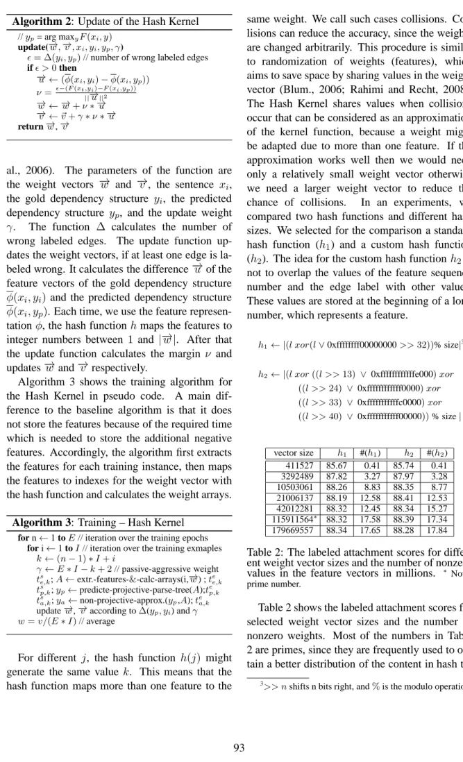
# Standard Features # Linear Features Linear G. Features Sibling Features 1 l,hf,hp,d(h,d) 14 l,hp,h+1p,dp,d(h,d) 44 l,gp,dp,d+1p,d(h,d) 99 l,sl,hp,d(h,d)⊕r(h,d) 2 l,hf,d(h,d) 15 l,hp,d-1p,dp,d(h,d) 45 l,gp,dp,d-1p,d(h,d) 100 l,sl,dp,d(h,d)⊕r(h,d) 3 l,hp,d(h,d) 16 l,hp,dp,d+1p,d(h,d) 46 l,gp,g+1p,d-1p,dp,d(h,d) 101 l,hl,dp,d(h,d)⊕r(h,d) 4 l,df,dp,d(h,d) 17 l,hp,h+1p,d-1p,dp,d(h,d) 47 l,g-1p,gp,d-1p,dp,d(h,d) 102 l,dl,sp,d(h,d)⊕r(h,d) 5 l,hp,d(h,d) 18 l,h-1p,h+1p,d-1p,dp,d(h,d) 48 l,gp,g+1p,dp,d+1p,d(h,d) 75 l,∀dm,∀sm,d(h,d) 6 l,dp,d(h,d) 19 l,hp,h+1p,dp,d+1p,d(h,d) 49 l,g-1p,gp,dp,d+1p,d(h,d) 76 l,∀hm,∀sm,d(h,s) 7 l,hf,hp,df,dp,d(h,d) 20 l,h-1p,hp,dp,d-1p,d(h,d) 50 l,gp,g+1p,hp,d(h,d) Linear S. Features 8 l,hp,df,dp,d(h,d) Grandchild Features 51 l,gp,g-1p,hp,d(h,d) 58 l,sp,s+1p,hp,d(h,d) 9 l,hf,df,dp,d(h,d) 21 l,hp,dp,gp,d(h,d,g) 52 l,gp,hp,h+1p,d(h,d) 59 l,sp,s-1p,hp,d(h,d) 10 l,hf,hp,df,d(h,d) 22 l,hp,gp,d(h,d,g) 53 l,gp,hp,h-1p,d(h,d) 60 l,sp,hp,h+1p,d(h,d) 11 l,hf,df,hp,d(h,d) 23 l,dp,gp,d(h,d,g) 54 l,gp,g+1p,h-1p,hp,d(h,d) 61 l,sp,hp,h-1p,d(h,d) 12 l,hf,df,d(h,d) 24 l,hf,gf,d(h,d,g) 55 l,g-1p,gp,h-1p,hp,d(h,d) 62 l,sp,s+1p,h-1p,d(h,d) 13 l,hp,dp,d(h,d) 25 l,df,gf,d(h,d,g) 56 l,gp,g+1p,hp,h+1p,d(h,d) 63 l,s-1p,sp,h-1p,d(h,d) 77 l,hl,hp,d(h,d) 26 l,gf,hp,d(h,d,g) 57 l,g-1p,gp,hp,h+1p,d(h,d) 64 l,sp,s+1p,hp,d(h,d) 78 l,hl,d(h,d) 27 l,gf,dp,d(h,d,g) Sibling Features 65 l,s-1p,sp,hp,h+1p,d(h,d) 79 l,hp,d(h,d) 28 l,hf,gp,d(h,d,g) 30 l,hp,dp,sp,d(h,d)⊕r(h,d) 66 l,sp,s+1p,dp,d(h,d) 80 l,dl,dp,d(h,d) 29 l,df,gp,d(h,d,g) 31 l,hp,sp,d(h,d)⊕r(h,d) 67 l,sp,s-1p,dp,d(h,d) 81 l,dl,d(h,d) 91 l,hl,gl,d(h,d,g) 32 l,dp,sp,d(h,d)⊕r(h,d) 68 sp,dp,d+1p,d(h,d) 82 l,dp,d(h,d) 92 l,dp,gp,d(h,d,g) 33 l,pf,sf,d(h,d)⊕r(h,d) 69 sp,dp,d-1p,d(h,d) 83 l,dl,hp,dp,hl,d(h,d) 93 l,gl,hp,d(h,d,g) 34 l,pp,sf,d(h,d)⊕r(h,d) 70 sp,s+1p,d-1p,dp,d(h,d) 84 l,dl,hp,dp,d(h,d) 94 l,gl,dp,d(h,d,g) 35 l,sf,pp,d(h,d)⊕r(h,d) 71 s-1p,sp,d-1p,dp,d(h,d) 85 l,hl,dl,dp,d(h,d) 95 l,hl,gp,d(h,d,g) 36 l,sf,dp,d(h,d)⊕r(h,d) 72 sp,s+1p,dp,d+1p,d(h,d) 86 l,hl,hp,dp,d(h,d) 96 l,dl,gp,d(h,d,g) 37 l,sf,dp,d(h,d)⊕r(h,d) 73 s-1p,sp,dp,d+1p,d(h,d) 87 l,hl,dl,hp,d(h,d) 74 l,∀dm,∀gm,d(h,d) 38 l,df,sp,d(h,d)⊕r(h,d) Special Feature

88 l,hl,dl,d(h,d) Linear G. Features 97 l,hl,sl,d(h,d)⊕r(h,d) 39 ∀l,hp,dp,xpbetween h,d

89 l,hp,dp,d(h,d) 42 l,gp,g+1p,dp,d(h,d) 98 l,dl,sl,d(h,d)⊕r(h,d)

41 l,_∀hm,∀dm,d(h,d) 43 l,gp,g-1p,dp,d(h,d)

Table 4: Features Groups. l represents the label, h the head, d the dependent, s a sibling, and g a grandchild, d(x,y,[,z]) the order of words, and r(x,y) the distance.

used cores. The parsing time is 1.9 times faster on two cores and 3.4 times faster on 4 cores. Hy-per threading can improve the parsing times again and we get with hyper threading 4.6 faster parsing times. Hyper threading possibly reduces the over-head of threads, which contains already our single core version.

Algorithm 4: Parallel Feature Extraction

A// weight arrays

extract-features-and-calc-arrays(xi)

data-list← {}// thread-save data list

forw1←1to|xi|

forw2←1to|xi|

data-list←data-list∪{(w1, w2)}

c←number of CPU cores

fort←1toc

Tt←create-array-thread(t, xi,data-list)

start array-threadTt// start thread t

fort_←1toc

joinTt// wait until threadtis finished

A_← A_∪collect-result(Tt)

returnA //

array-threadT

d_←remove-first-element(data-list)

ifdis empty then end-thread

... // extract features and calculate partdofA

Cores te tp ta rest total pars. train.

1 379 21.3 18.2 1.5 420 354 45.8h

2 196 11.7 9.2 2.1 219 187 23.9h

3 138 8.9 6.5 1.6 155 126 16.6h

4 106 8.2 5.2 1.6 121 105 13.2h

4+4h 73.3 8.8 4.8 1.3 88.2 77 9.6h

Table 5: Elapsed times in milliseconds for differ-ent numbers of cores. The parsing time (pars.) are expressed in milliseconds per sentence and the training (train.) time in hours. The last row shows the times for 8 threads on a 4 core CPU with Hyper-threading. For these experiment, we set the clock speed to 3.46 Ghz in order to have the same clock speed for all experiments.

6 Non-Projective Approximation Threshold

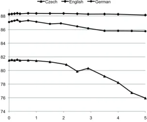
For non-projective parsing, we use the Non-Projective Approximation Algorithm of McDon-ald and Pereira (2006). The algorithm rearranges edges in a dependency tree when they improve the score. Bohnet (2009) extended the algorithm by a threshold which biases the rearrangement of the edges. With a threshold, it is possible to gain a higher percentage of correct dependency links. We determined a threshold in experiments for Czech, English and German. In the experiment, we use the Hash Kernel and increase the

thresh-System Average Catalan Chinese Czech English German Japanese Spanish Top CoNLL 09 85.77(1) 87.86(1) 79.19(4) 80.38(1) 89.88(2) 87.48(2) 92.57(3) 87.64(1)

Baseline Parser 85.10 85.70 76.88 76.93 90.14 87.64 92.26 86.12

this work 86.33 87.45 76.99 80.96 90.33 88.06 92.47 88.13

Table 6: Top LAS of the CoNLL 2009 of (1) Gesmundo et al. (2009), (2) Bohnet (2009), (3) Che et al. (2009), and (4) Ren et al. (2009); LAS of the baseline parser and the parser with Hash Kernel. The numbers in bold face mark the top scores. We used for Catalan, Chinese, Japanese and Spanish the projective parsing algorithm.

old at the beginning in small steps by 0.1 and later in larger steps by 0.5 and 1.0. Figure 2 shows the labeled attachment scores for the Czech, En-glish and German development set in relation to the rearrangement threshold. The curves for all languages are a bit volatile. The English curve is rather flat. It increases a bit until about 0.3 and remains relative stable before it slightly de-creases. The labeled attachment score for Ger-man and Czech increases until 0.3 as well and then both scores start to decrease. For English a thresh-old between 0.3 and about 2.0 would work well. For German and Czech, a threshold of about 0.3 is the best choice. We selected for all three lan-guages a threshold of 0.3. 74 76 78 80 82 84 86 88 0 1 2 3 4 5

Czech English German

Figure 2: English, German, and Czech labeled at-tachment score (y-axis) for the development set in relation to the rearrangement threshold (x-axis). 7 Conclusion and Future Work

We have developed a very fast parser with ex-cellent attachment scores. For the languages of the 2009 CoNLL Shared Task, the parser could reach higher accuracy scores on average than the top performing systems. The scores for Catalan, Chinese and Japanese are still lower than the top

scores. However, the parser would have ranked second for these languages. For Catalan and Chinese, the top results obtained transition-based parsers. Therefore, the integration of both tech-niques as in Nivre and McDonald (2008) seems to be very promising. For instance, to improve the accuracy further, more global constrains cap-turing the subcategorization correct could be inte-grated as in Riedel and Clarke (2006). Our faster algorithms may make it feasible to consider fur-ther higher order factors.

In this paper, we have investigated possibilities for increasing parsing speed without any accuracy loss. The parsing time is 3.5 times faster on a sin-gle CPU core than the baseline parser which has an typical architecture for a maximum spanning tree parser. The improvement is due solely to the Hash Kernel. The Hash Kernel was also a prereq-uisite for the parallelization of the parser because it requires much less memory bandwidth which is nowadays a bottleneck of parsers and many other applications.

By using parallel algorithms, we could further increase the parsing time by a factor of 3.4 on a 4 core CPU and including hyper threading by a factor of 4.6. The parsing speed is 16 times faster for the English test set than the conventional ap-proach. The parser needs only 77 millisecond in average to parse a sentence and the speed will scale with the number of cores that become avail-able in future. To gain even faster parsing times, it may be possible to trade accuracy against speed. In a pilot experiment, we have shown that it is possible to reduce the parsing time in this way to as little as 9 milliseconds. We are convinced that the Hash Kernel can be applied successful to tran-sition based dependency parsers, phrase structure parsers and many other NLP applications.4

4

We provide the Parser and Hash Kernel as open source for download from http://code.google.com/p/mate-tools.

References

Attardi, G. 2006. Experiments with a Multilanguage Non-Projective Dependency Parser. In Proceedings

of CoNLL, pages 166–170.

Blum., A. 2006. Random Projection, Margins, Ker-nels, and Feature-Selection. In LNCS, pages 52–68. Springer.

Bohnet, B. 2009. Efficient Parsing of Syntactic and Semantic Dependency Structures. In Proceedings

of the 13th Conference on Computational Natural Language Learning (CoNLL-2009).

Carreras, X. 2007. Experiments with a Higher-order Projective Dependency Parser. In EMNLP/CoNLL. Che, W., Li Z., Li Y., Guo Y., Qin B., and Liu T. 2009.

Multilingual Dependency-based Syntactic and Se-mantic Parsing. In Proceedings of the 13th

Confer-ence on Computational Natural Language Learning (CoNLL-2009).

Collins, M. 2002. Discriminative Training Methods for Hidden Markov Models: Theory and Experi-ments with Perceptron Algorithms. In EMNLP. Crammer, K., O. Dekel, S. Shalev-Shwartz, and

Y. Singer. 2003. Online Passive-Aggressive Algo-rithms. In Sixteenth Annual Conference on Neural

Information Processing Systems (NIPS).

Crammer, K., O. Dekel, S. Shalev-Shwartz, and Y. Singer. 2006. Online Passive-Aggressive Al-gorithms. Journal of Machine Learning Research, 7:551–585.

Eisner, J. 1996. Three New Probabilistic Models for Dependency Parsing: An Exploration. In

Proceed-ings of the 16th International Conference on Com-putational Linguistics (COLING-96), pages 340–

345, Copenhaen.

Eisner, J., 2000. Bilexical Grammars and their

Cubic-time Parsing Algorithms, pages 29–62. Kluwer Academic Publishers.

Gesmundo, A., J. Henderson, P. Merlo, and I. Titov. 2009. A Latent Variable Model of Syn-chronous Syntactic-Semantic Parsing for Multiple Languages. In Proceedings of the 13th

Confer-ence on Computational Natural Language Learning (CoNLL-2009), Boulder, Colorado, USA., June 4-5.

Hajiˇc, J., M. Ciaramita, R. Johansson, D. Kawahara, M. Ant`onia Mart´ı, L. M`arquez, A. Meyers, J. Nivre, S. Pad ´o, J. ˇStˇep´anek, P. Straˇn´ak, M. Surdeanu, N. Xue, and Y. Zhang. 2009. The CoNLL-2009 Shared Task: Syntactic and Semantic Dependencies in Multiple Languages. In Proceedings of the 13th

CoNLL-2009, June 4-5, Boulder, Colorado, USA.

Johansson, R. and P. Nugues. 2008. Dependency-based Syntactic–Semantic Analysis with PropBank and NomBank. In Proceedings of the Shared Task

Session of CoNLL-2008, Manchester, UK.

McDonald, R. and F. Pereira. 2006. Online Learning of Approximate Dependency Parsing Algorithms. In In Proc. of EACL, pages 81–88.

McDonald, R., K. Crammer, and F. Pereira. 2005. On-line Large-margin Training of Dependency Parsers. In Proc. ACL, pages 91–98.

Nivre, J. and R. McDonald. 2008. Integrating Graph-Based and Transition-Graph-Based Dependency Parsers. In ACL-08, pages 950–958, Columbus, Ohio. Nivre, J., J. Hall, and J. Nilsson. 2004.

Memory-Based Dependency Parsing. In Proceedings of the

8th CoNLL, pages 49–56, Boston, Massachusetts.

Nivre, J. 2003. An Efficient Algorithm for Pro-jective Dependency Parsing. In 8th International

Workshop on Parsing Technologies, pages 149–160,

Nancy, France.

Nivre, J. 2009. Non-Projective Dependency Parsing in Expected Linear Time. In Proceedings of the 47th

Annual Meeting of the ACL and the 4th IJCNLP of the AFNLP, pages 351–359, Suntec, Singapore.

Rahimi, A. and B. Recht. 2008. Random Features for Large-Scale Kernel Machines. In Platt, J.C., D. Koller, Y. Singer, and S. Roweis, editors,

Ad-vances in Neural Information Processing Systems,

volume 20. MIT Press, Cambridge, MA.

Ren, H., D. Ji Jing Wan, and M. Zhang. 2009. Pars-ing Syntactic and Semantic Dependencies for Mul-tiple Languages with a Pipeline Approach. In

Pro-ceedings of the 13th Conference on Computational Natural Language Learning (CoNLL-2009),

Boul-der, Colorado, USA., June 4-5.

Riedel, S. and J. Clarke. 2006. Incremental Inte-ger Linear Programming for Non-projective Depen-dency Parsing. In Proceedings of the 2006

Con-ference on Empirical Methods in Natural Language Processing, pages 129–137, Sydney, Australia, July.

Association for Computational Linguistics.

Shi, Q., J. Petterson, G. Dror, J. Langford, A. Smola, and S.V.N. Vishwanathan. 2009. Hash Kernels for Structured Data. In Journal of Machine Learning. Titov, I. and J. Henderson. 2007. A Latent Variable

Model for Generative Dependency Parsing. In

Pro-ceedings of IWPT, pages 144–155.

Yamada, H. and Y. Matsumoto. 2003. Statistical De-pendency Analysis with Support Vector Machines. In Proceedings of IWPT, pages 195–206.