A Bayesian Variable Selection Approach Yields Improved Detection of Brain Activation From Complex-Valued fMRI

Marquette University

e-Publications@Marquette

Mathematics, Statistics and Computer Science

Faculty Research and Publications

Mathematics, Statistics and Computer Science,

Department of (-2019)

1-1-2018

A Bayesian Variable Selection Approach Yields

Improved Detection of Brain Activation From

Complex-Valued f MRI

Cheng-Han Yu

University of California - Santa Cruz

Raquel Prado

University of California - Santa Cruz

Hernando Ombao

King Abdullah University of Science and Technology

Daniel B. Rowe

Marquette University, [email protected]

Accepted version.

Journal of the American Statistical Association, Vol. 113, No. 524 (2018):

1395-1410.

DOI. © 2018 Taylor & Francis. Used with permission.

Marquette University

e-Publications@Marquette

Mathematics and Statistical Sciences Faculty Research and

Publications/College of Arts and Sciences

This paper is NOT THE PUBLISHED VERSION;

but the author’s final, peer-reviewed manuscript.

The

published version may be accessed by following the link in th citation below.

Journal of the American Statistical Association

, Vol. 113, No. 524 (2018): 1395-1410.

DOI

. This article is

© Taylor & Francis and permission has been granted for this version to appear in

e-Publications@Marquette

. Taylor & Francis does not grant permission for this article to be further

copied/distributed or hosted elsewhere without the express permission from Taylor & Francis.

A Bayesian Variable Selection Approach Yields Improved

Detection of Brain Activation From Complex-Valued fMRI

Cheng-Han Yu

Department of Applied Mathematics & Statistics, University of California at Santa Cruz, Santa Cruz, CA

Raquel Prado

Department of Applied Mathematics & Statistics, University of California at Santa Cruz, Santa Cruz, CA

Hernando Ombao

Statistics Program, King Abdullah University of Science and Technology (KAUST), Saudi Arabia

Daniel Rowe

Department of Mathematics, Statistics and Computer Science, Marquette University, Milwaukee, WI

Abstract

Voxel functional magnetic resonance imaging (fMRI) time courses are complex-valued signals giving rise to

magnitude and phase data. Nevertheless, most studies use only the magnitude signals and thus discard half of the data that could potentially contain important information. Methods that make use of complex-valued fMRI (CV-fMRI) data have been shown to lead to superior power in detecting active voxels when compared to magnitude-only methods, particularly for small signal-to-noise ratios (SNRs). We present a new Bayesian variable selection approach for detecting brain activation at the voxel level from CV-fMRI data. We develop models with complex-valued spike-and-slab priors on the activation parameters that are able to combine the magnitude and phase information. We present a complex-valued EM variable selection algorithm that leads to fast detection at the voxel level in CV-fMRI slices and also consider full posterior inference via Markov chain Monte Carlo (MCMC).

Model performance is illustrated through extensive simulation studies, including the analysis of physically based simulated CV-fMRI slices. Finally, we use the complex-valued Bayesian approach to detect active voxels in human CV-fMRI from a healthy individual who performed unilateral finger tapping in a designed experiment. The

proposed approach leads to improved detection of activation in the expected motor-related brain regions and produces fewer false positive results than other methods for CV-fMRI. Supplementary materials for this article are available online.

Keywords:

Bayesian modeling, Complex-valued time series, CV-fMRI, Variable selection

1. Introduction

As an imaging modality, fMRI is able to indirectly measure neuronal activity by detecting changes in the blood oxygen level dependent (BOLD) signal. In a typical task-related fMRI experiment, hemodynamic activity over the entire brain volume is observed at T time points while a subject performs a series of tasks, leading to a set of T large-dimensional fMRI scans, typically T rectangular lattices with about 5K–10K voxels.

In MRI and fMRI, images or voxel measurements are complex-valued due to phase imperfections after Fourier encoding and inverse Fourier image reconstruction. Thus in fMRI, voxel time course measurements consist of real and imaginary components (Bernstein, Thomasson, and Perman

1989

; Macovski

1996

; Haacke et al.

1999

) and these are generally converted to magnitude and phase voxel time courses. However, most fMRI brain activation studies discard the phase information and rely on magnitude-only image time courses. When this is done, the original complex-valued data are unrecoverable as operations that involve magnitude-only reconstruction are not unique. Some attempts have been made to avoid working with complex-valued voxel time courses or standard magnitude-based reconstruction algorithms. For instance, Bernstein, Thomasson, and Perman (

1989

) and Prah et al. (

2010

) showed that detectability in low signal-to-noise (SNR) regions of magnetic resonance images is improved by using a phase-corrected real reconstruction instead of magnitude-only reconstructions. In this article, we develop a Bayesian model for detecting activation that uses both the real and imaginary components in CV-fMRI data, leading to more accurate activation results.

Bandettini et al. (

1992

) demonstrated that voxel time courses can be used as effective tools for localizing brain function in humans. Early common model-based approaches to the analysis of magnitude fMRI data relied on the general linear model (GLM), as first proposed by Friston, Jezzard, and Turner (

1994

). In this model, the observed magnitude-only fMRI signal is modeled as the underlying expected BOLD response plus a noise component. In other words, for each voxel v = 1, …, V, the voxel-wise GLM can be written as

y

𝑣𝑣

=

X

𝑣𝑣

𝛃𝛃

𝑣𝑣

+

𝛜𝛜

𝑣𝑣

,

(1)

where  yv is the T × 1 response vector of magnitude-only fMRI time course for voxel v,  Xv is the T × q design matrix

whose components include the expected BOLD responses for each of p experimental tasks or input stimuli and possibly other regressors such as trends (and so, p⩽q),

𝛃𝛃

𝑣𝑣 is a q × 1 vector of regression coefficients and

𝛜𝛜

𝑣𝑣

is

a T × 1 error vector, which captures random noises due to scanner artifacts and any additional subject-related physiological noise. In the absence of intercepts, trends, or any other covariates that are not task-specific, that is, when q = p, each of the p BOLD responses in  Xv is the discretized convolution of a stimulus on-and-off signal with

the so-called hemodynamic response function (HRF) that models the hemodynamic delay in the magnetic resonance signal (Friston et al.

2007

). In addition, the HRF is often assumed to be the same across voxels, resulting in  Xv =  X for all v.

Sophisticated Bayesian models, including spatial and spatio-temporal approaches, have been developed for magnitude-only fMRI data. For instance, Bowman et al. (

2008

) considered a two-stage Bayesian hierarchical model with temporal correlations at the first stage and spatial correlations at the second stage. In Lee et al. (

2014

), temporal dependence is characterized via autoregressive models, Zellner’s g-priors are assumed for the regression coefficients, and a binary spatial Ising prior is used to specify anatomical information and spatial interaction between voxels. In Zhang et al. (

2014

), a general error structure is used to capture general dependence, and a Markov random field (MRF) prior is used to detect activations in a nonparametric way. Alternative Bayesian approaches for magnitude-only data are summarized in Zhang, Guindani, and Vannucci (

2015

), Zhang et al. (

2016

), and Chiang et al. (

2017

). These sophisticated and well-constructed models, however, are based only on the magnitude information provided by the data and do not incorporate the phase information. Furthermore, many of these magnitude-only approaches also work under the assumption that the errors are normally distributed which may be problematic, resulting in incorrect standard errors that can produce inaccurate activation results. In fact, if both the real and imaginary components of the CV-fMRI signals have independent normally distributed errors with the same variance, the magnitude-only signals actually follow a Ricean distribution that is approximately normal only in the case of large SNRs (Rice

1944

; Gudbjartsson and Patz

1995

; Rowe and Logan

2004

). However, the SNRs may not be large enough in practice for this approximate normality to hold. This is increasingly true in cases with higher voxel resolutions and for voxels with a large degree of signal drop-out, that is, those for which the signal is not available or has small SNR, such as voxels located near air/tissue boundaries. In particular, Adrian, Maitra, and Rowe (

2013

) showed that with magnitude-only models, tests derived using Ricean modeling are superior to Gaussian-based activation tests for SNRs below 0.6. Rowe (

2005b

) also showed that Gaussian-based activation parameter estimates were biased for SNRs under 10. Our approach overcomes these limitations of magnitude-only models by jointly considering the real and imaginary components of CV-fMRI data.

Complex-valued modeling has been widely used in several applied areas allowing full utilization of real and imaginary, or equivalently magnitude and phase, information in certain signals and images, providing a general framework for the analysis of several classes of processes (see, e.g., Mandic and Goh,

2009

). The incorporation of phase information has proven key in communications and imaging (Oppenheim and Lim

1981

), as complex-valued modeling simultaneously handles the intensity and direction when dealing with radar, sonar, and wind data. In the fMRI context, CV-fMRI data that jointly consist of magnitude and phase images are not provided by the scanners as the default output, but they are usually readily available. For instance, GE scanners typically provide an output file that contains the raw complex-valued k-space data and other information, as well as the magnitude images. Magnitude and phase images, or real and imaginary images, can be easily obtained by simply changing a preset control variable in an input file, making CV-fMRI data available to neuroimaging researchers and practitioners.

A number of tools for CV-fMRI data analysis have been proposed in the literature, including nonmodel-based exploratory independent component analysis (ICA; Calhoun et al.

2002

), as well as direct modeling of the complex activation data (Lai and Glover

1997

; Rowe and Logan

2004

,

2005

; Rowe

2005a

; Lee et al.

2007

; Rowe

2009

; Lee, Shahram, and Pauly

2009

). Approaches such as those in Rowe and Logan (

2004

,

2005

); Rowe (

2005a

); and Rowe (

2005b

) model the phase to directly estimate the phase angle using a polar coordinates representation, while the methods in Lee et al. (

2007

) and Lee, Shahram, and Pauly (

2009

) are based on Cartesian representations. More recently, complex-valued models with temporal correlations (including

autoregressive structures) have also been developed (Kociuba and Rowe

2016

; Adrian, Maitra, and Rowe

2017

). In particular, Rowe (

2005a

) specified the following structure for the complex-valued image measurement at time t and voxel v,

𝑦𝑦

𝑡𝑡

𝑣𝑣

=

𝑦𝑦

𝑡𝑡

𝑣𝑣

,

𝑅𝑅𝑅𝑅

+

𝑖𝑖𝑦𝑦

𝑡𝑡

𝑣𝑣

,

𝐼𝐼𝐼𝐼

∈ ℂ

,

𝑦𝑦

𝑡𝑡

𝑣𝑣

=

𝜌𝜌

𝑡𝑡

𝑣𝑣

𝑐𝑐𝑐𝑐𝑐𝑐

(

𝜙𝜙

𝑡𝑡

𝑣𝑣

) +

𝑖𝑖𝜌𝜌

𝑡𝑡

𝑣𝑣

𝑐𝑐𝑖𝑖𝑠𝑠

(

𝜙𝜙

𝑡𝑡

𝑣𝑣

) +

𝜂𝜂

𝑡𝑡

𝑣𝑣

,

(2)

where

𝜌𝜌

_𝑡𝑡𝑣𝑣

=

𝛽𝛽

₀𝑣𝑣

+

𝛽𝛽

₁𝑣𝑣

𝑥𝑥

_1,𝑡𝑡

+

⋯

+

𝛽𝛽

_𝑝𝑝𝑣𝑣₁

𝑥𝑥

_{𝑝𝑝1,𝑡𝑡} is the magnitude of yvt with p1 magnitude regressors, 𝜙𝜙_𝑡𝑡𝑣𝑣=

𝛼𝛼0𝑣𝑣+𝛼𝛼1𝑣𝑣𝑢𝑢1,𝑡𝑡+⋯+𝛼𝛼𝑝𝑝𝑣𝑣2𝑢𝑢𝑝𝑝2,𝑡𝑡is the phase of yvt with p2 regressors, and 𝑖𝑖=√−1.

.

All the regression coefficients βv0, …, βp1vand αv0, …, αp2v are real-valued. Here, aRe and aIm generically denote the real and imaginary parts of any

complex-valued quantity a = aRe + iaIm. The noise term ηvt is also assumed to be complex-valued, that is, ηvt =

ηt, Rev + iηvt, Im. When αv0≠ 0 and αvj = 0 for all j = 1, …, p2, we have the Rowe-Logan constant phase model. Note that

when no trends are included, the magnitude and phase regressors could be chosen to be identical to the expected bold responses associated with the p experimental tasks, that is, p1 = p2 = p and xj, t = uj, t for all j = 1, …, p. Rowe

(

2005a

) identified active voxels using a generalized likelihood ratio test.

Lee et al. (

2007

) and Lee, Shahram, and Pauly (

2009

) proposed a method based on a Cartesian model representation which has the following matrix form:

y

𝑣𝑣

=

X

𝛄𝛄

𝑣𝑣

+

𝛈𝛈

𝑣𝑣

,

(3)

with  yv _{= (y}v_{1,…, yT}v_{)′, 𝛄𝛄}𝑣𝑣_=𝛄𝛄 𝑅𝑅𝑅𝑅 𝑣𝑣 _{+𝑖𝑖𝛄𝛄} 𝐼𝐼𝐼𝐼 𝑣𝑣 _,𝛄𝛄 𝑅𝑅𝑅𝑅 𝑣𝑣 _{= (𝛾𝛾} 𝑅𝑅𝑅𝑅𝑣𝑣 ,1, … ,𝛾𝛾𝑅𝑅𝑅𝑅𝑣𝑣 ,𝑞𝑞)′, 𝛄𝛄𝐼𝐼𝐼𝐼𝑣𝑣 = (𝛾𝛾𝐼𝐼𝐼𝐼𝑣𝑣 ,1, … ,𝛾𝛾𝐼𝐼𝐼𝐼𝑣𝑣 ,𝑞𝑞)′, with q = p + 1,  X = (x′1,

…, xT′)′, wherext = (1, x1, t, …, xp, t)′,t = 1, …, T, and complex-valued noise vector 𝛈𝛈𝑣𝑣= (𝜂𝜂₁𝑣𝑣, … ,𝜂𝜂_𝑇𝑇𝑣𝑣).. Lee et al. (2007)

combined this general linear model representation in Cartesian coordinates with a Hotelling’s T2_{-test to detect}

active sites. Model (3) is equivalent to the Rowe–Logan constant phase complex-valued model (Rowe and

Logan 2004) if p1 = p, 𝛄𝛄_{𝑅𝑅𝑅𝑅}𝑣𝑣 =�𝛽𝛽₀𝑣𝑣, … ,𝛽𝛽_𝑝𝑝𝑣𝑣�′𝑐𝑐𝑐𝑐𝑐𝑐(𝛼𝛼₀𝑣𝑣) and 𝛄𝛄_{𝐼𝐼𝐼𝐼}𝑣𝑣 = (𝛽𝛽₀𝑣𝑣, … ,𝛽𝛽_𝑝𝑝𝑣𝑣)′𝑐𝑐𝑖𝑖𝑠𝑠(𝛼𝛼₀𝑣𝑣).. Model (3) is also equivalent to

the complex-valued magnitude and phase activation model in Rowe and Logan (2005) when there is only a single regressor in both, magnitude and phase, corresponding to a 0/1 vector representing a boxcar block design. The references cited above show that modeling the complete CV-fMRI data leads to superior power in detecting active voxels when compared to magnitude-only approaches, especially for situations in which the SNRs are relatively small. However, in spite of their advantages, currently available methods for CV-fMRI data rely on mechanisms that control some notion of error to correct for multiple testing, such as Bonferroni corrections, and therefore involve two-step procedures. The first step provides estimates of the potentially active voxels according to some model, while the second step involves using one of the standard methods to correct for multiple testing. Furthermore, available methods for CV-fMRI data assume that the voxels are independent and do not offer a principled framework for parameter learning through borrowing information across voxels.

Here, we present a Bayesian approach that allows us to infer active voxels using both the real and imaginary information provided by the CV-fMRI data. This approach builds on Bayesian variable selection methods to detect active voxels and hence does not suffer from the multiple comparison issues that typically affect multiple

hypothesis testing (Scott and Berger 2006). Activation detection and parameter estimation are achieved by a model-based framework that allows us to borrow information across voxels. In addition to obtaining full posterior inference via Markov chain Monte Carlo (MCMC), we develop a complex-valued extension of the Expectation-Maximization (EM) algorithm for Bayesian variable selection of Rockova and George (2014) that allows for fast detection of active voxels in large-dimensional CV-fMRI. The advantages of our approach are illustrated in the analysis of simulated data, including physically realistic simulated CV-fMRI data, as well as human CV-fMRI data. We show that the proposed methods lead to more accurate activation results than those obtained from

magnitude-only methods or from currently available methods for CV-fMRI data. Section

2

presents the models and algorithms for posterior estimation and inference. Section

3

illustrates the performance of the Bayesian

approach for detecting active voxels in simulated datasets, including physically realistic synthetic CV-fMRI data. Section

4

shows and discusses the results obtained from analyzing a human CV-fMRI dataset with the proposed Bayesian approach. Finally, Section

5

presents a discussion and future extensions.

2. Bayesian Models for Detecting Activation in Complex-Valued fMRI Data

As mentioned above, we develop a model that makes use of the complete magnitude and phase information provided by the CV-fMRI data. However, unlike previous approaches (Rowe and Logan 2004, 2005;

Rowe 2005a, 2009; Lee et al. 2007), we use a fully Bayesian framework for identifying active voxels via variable selection in the complex-valued domain.

We follow the Cartesian coordinates approach of Lee et al. (2007) given in (3) and further assume independent and identically distributed complex-normal error vectors, that is,

y

𝑣𝑣

=

X

𝛄𝛄

𝑣𝑣

+

𝛈𝛈

𝑣𝑣

,

𝛈𝛈

𝑣𝑣

∼

CN

𝑇𝑇

(

𝟎𝟎

,

𝚪𝚪

𝑣𝑣

,

C

𝑣𝑣

),

(4)

with CN𝐿𝐿(𝛍𝛍,𝚪𝚪,C) denoting a complex normal distribution of dimension L with mean 𝛍𝛍, complex-valued, Hermitian

and nonnegative definite covariance matrix 𝚪𝚪, and complex-valued symmetric relation matrix  C. As shown below, the linear structure in this representation is computationally relevant, as it leads to fast Bayesian posterior estimation of active sites. Note also that any complex-valued normal distribution of dimension L has a real-valued normal representation of dimension 2L (Wooding 1956; van den Bos 1995; Picinbono 1996 Pici). Thus,

letting 𝚺𝚺𝑅𝑅𝑅𝑅𝑣𝑣 ,𝑅𝑅𝑅𝑅 =1₂𝑅𝑅𝑅𝑅(𝚪𝚪𝑣𝑣+C𝑣𝑣),𝚺𝚺𝐼𝐼𝐼𝐼𝑣𝑣 ,𝐼𝐼𝐼𝐼=1₂𝑅𝑅𝑅𝑅(𝚪𝚪𝑣𝑣−C𝑣𝑣),𝚺𝚺𝑅𝑅𝑅𝑅𝑣𝑣 ,𝐼𝐼𝐼𝐼 =1₂𝐼𝐼𝐼𝐼(−𝚪𝚪𝑣𝑣+C𝑣𝑣), and 𝚺𝚺𝐼𝐼𝐼𝐼𝑣𝑣 ,𝑅𝑅𝑅𝑅 =1₂𝐼𝐼𝐼𝐼(𝚪𝚪𝑣𝑣+

C_𝑣𝑣), model (4) also has a real-valued representation as

�

y

y

𝑅𝑅𝑅𝑅

𝑣𝑣

𝐼𝐼𝐼𝐼

𝑣𝑣

�

=

�

𝟎𝟎

X

𝟎𝟎

X

� �

𝛄𝛄

𝑅𝑅𝑅𝑅

𝑣𝑣

𝛄𝛄

𝐼𝐼𝐼𝐼

𝑣𝑣

�

+

� 𝛈𝛈

𝑅𝑅𝑅𝑅

𝑣𝑣

𝛈𝛈

𝐼𝐼𝐼𝐼

𝑣𝑣

,

�

,

(5)

or equivalently,

y

𝑟𝑟

𝑣𝑣

=

X

𝑟𝑟

𝛄𝛄

𝑟𝑟

𝑣𝑣

+

𝛈𝛈

𝑟𝑟

𝑣𝑣

,

(6)

with  yv

r = (( yRev)′, ( yvIm)′)′,  Xr = blockdiag( X,  X), 𝛄𝛄_𝑟𝑟𝑣𝑣= ((𝛄𝛄_{𝑅𝑅𝑅𝑅}𝑣𝑣 )′, (𝛄𝛄_{𝐼𝐼𝐼𝐼}𝑣𝑣 )′)′, and 𝛈𝛈_𝑟𝑟𝑣𝑣 = ((𝛈𝛈_{𝑅𝑅𝑅𝑅}𝑣𝑣 )′, (𝛈𝛈_{𝐼𝐼𝐼𝐼}𝑣𝑣 )′)′, where 𝛈𝛈_𝑟𝑟𝑣𝑣∼

𝑁𝑁2𝑇𝑇(𝟎𝟎,𝛴𝛴𝑣𝑣) with

𝛴𝛴

𝑣𝑣

=

�

𝚺𝚺

𝚺𝚺

𝑅𝑅𝑅𝑅

𝑣𝑣

,

𝑅𝑅𝑅𝑅

𝚺𝚺

𝑅𝑅𝑅𝑅

𝑣𝑣

,

𝐼𝐼𝐼𝐼

𝐼𝐼𝐼𝐼

,

𝑅𝑅𝑅𝑅

𝑣𝑣

𝚺𝚺

𝐼𝐼𝐼𝐼

,

𝐼𝐼𝐼𝐼

𝑣𝑣

�

.

The simplest possible structure for 𝛈𝛈𝑣𝑣 _{is that obtained by taking 𝛈𝛈}𝑣𝑣_∼CN

𝑇𝑇(𝟎𝟎, 2𝜎𝜎𝑣𝑣2I𝑇𝑇,𝟎𝟎) or equivalently,

setting 𝛴𝛴𝑣𝑣=𝜎𝜎𝑣𝑣2I2𝑇𝑇 in the real-valued Gaussian representation. This implies that there is no correlation within the

real components and within the imaginary components of 𝛈𝛈𝑣𝑣_{, and also that there is no correlation between the}

real and imaginary components of 𝛈𝛈𝑣𝑣_{. These assumptions can be relaxed to include correlations within the real}

and imaginary components to capture temporal structure (as illustrated in some of the analysis of synthetic and human CV-fMRI data presented in Sections 3 and 4), or correlations between the real and imaginary components for more structured noise.

Below we describe the priors and the corresponding posterior inference for the simplest noise structure, focusing on complex-valued priors for 𝛄𝛄𝑣𝑣 _{that lead to posterior inference of activation in CV-fMRI at the voxel-specific}

2.1. Priors

In the absence of any trends and intercepts, and without loss of generality, that is, for the case in which  X in (4) contains only the expected BOLD signals for each of p stimuli/tasks with no baselines or trends, activation can be viewed as a variable selection problem (Xia, Liang, and Wang 2009; Zhang, Guindani, and Vannucci 2015). In other words, if γv

j= γRe, jv + iγvIm, j≠ 0 for voxelv and task j, such voxel is identified as active under task j. Note that

complex-valued priors must be considered for γv

j. Here we develop a complex-valued domain analogue of the

Bayesian variable selection methods of George and McCulloch (1993, 1997) and Rockova and George (2014). If trends and/or intercepts are needed, they can easily be included in the model along with priors on their

corresponding parameters and integrated out, as done in the applications illustrated in Sections 3 and 4. Thus, we focus the discussion below to the case in which  X only consists of the expected BOLD signals associated with each of the p experimental stimuli/tasks.

Our proposed complex-valued spike-and-slab priors for γv_{j extend the widely used real-valued spike-and-slab}

priors by considering

�𝛾𝛾

_𝑗𝑗𝑣𝑣

|

𝜓𝜓

_𝑗𝑗𝑣𝑣

� ∼ �

1

−𝜓𝜓

_𝑗𝑗𝑣𝑣

�𝑔𝑔

0

�𝛾𝛾

𝑗𝑗𝑣𝑣

�

+

𝜓𝜓

𝑗𝑗𝑣𝑣

𝑔𝑔�𝛾𝛾

𝑗𝑗𝑣𝑣

�

,

with g0( · ) and g( · ) complex-valued distributions with mean zero, and ψvj∈{0, 1}, where ψvj = 1 indicates that

voxel v is active during task j. Therefore, this prior allows us to determine if a voxel is active by jointly considering the real and imaginary components of γvj. In general, we consider priors with g0(γvj) = CN1(0, σ2vω0, σ2vλ0), and g(γvj)

= CN1(0, σ2vω1, σ2vλ1), and their corresponding vectorial representation given by

𝛄𝛄

𝑣𝑣

|

𝛙𝛙

𝑣𝑣

∼ 𝐶𝐶𝑁𝑁

𝑝𝑝

(

𝟎𝟎

,

𝜎𝜎

𝑣𝑣2

𝛀𝛀

𝑣𝑣

,

𝜎𝜎

𝑣𝑣2

𝚲𝚲

𝑣𝑣

),

(7)

with 𝛀𝛀𝑣𝑣=diag�(1− 𝜓𝜓1𝑣𝑣)𝜔𝜔0+𝜓𝜓1𝑣𝑣𝜔𝜔1, … ,�1− 𝜓𝜓𝑝𝑝𝑣𝑣�𝜔𝜔0+𝜓𝜓𝑝𝑝𝑣𝑣𝜔𝜔1�, 𝚲𝚲𝑣𝑣=diag((1− 𝜓𝜓1𝑣𝑣)𝜆𝜆0+𝜓𝜓1𝑣𝑣𝜆𝜆1, … , (1−

𝜓𝜓𝑝𝑝𝑣𝑣)𝜆𝜆0+𝜓𝜓𝑝𝑝𝑣𝑣𝜆𝜆1) and 𝛙𝛙𝑣𝑣= [𝜓𝜓1𝑣𝑣, … ,𝜓𝜓𝑝𝑝𝑣𝑣]. The real-valued representation of this prior is �𝛄𝛄𝑅𝑅𝑅𝑅 𝑣𝑣 𝛄𝛄𝐼𝐼𝐼𝐼𝑣𝑣 � ∼ 𝑁𝑁2𝑝𝑝�𝟎𝟎,𝜎𝜎𝑣𝑣2𝛴𝛴(𝛙𝛙𝑣𝑣)�, where 𝛴𝛴(𝛙𝛙𝑣𝑣) =�𝛴𝛴𝑅𝑅𝑅𝑅,𝑅𝑅𝑅𝑅(𝛙𝛙 𝑣𝑣_{) 𝛴𝛴} 𝑅𝑅𝑅𝑅,𝐼𝐼𝐼𝐼(𝛙𝛙𝑣𝑣) 𝛴𝛴𝐼𝐼𝐼𝐼,𝑅𝑅𝑅𝑅(𝛙𝛙𝑣𝑣) 𝛴𝛴𝐼𝐼𝐼𝐼,𝐼𝐼𝐼𝐼(𝛙𝛙𝑣𝑣)�. Given 𝛙𝛙 𝑣𝑣_{, we} obtain 𝛴𝛴(𝛙𝛙𝑣𝑣_{) from 𝛀𝛀} 𝑣𝑣 and 𝚲𝚲𝑣𝑣 via 𝛴𝛴𝑅𝑅𝑅𝑅,𝑅𝑅𝑅𝑅(𝛙𝛙𝑣𝑣) =1₂𝑅𝑅𝑅𝑅(𝛀𝛀𝑣𝑣+𝛴𝛴𝐼𝐼𝐼𝐼,𝐼𝐼𝐼𝐼(𝛙𝛙𝑣𝑣) =1₂𝑅𝑅𝑅𝑅(𝛀𝛀𝑣𝑣− 𝚲𝚲𝑣𝑣), 𝛴𝛴𝑅𝑅𝑅𝑅,𝐼𝐼𝐼𝐼(𝛙𝛙𝑣𝑣) = 1 2𝐼𝐼𝐼𝐼(−𝛀𝛀𝑣𝑣+𝚲𝚲𝑣𝑣), and 𝛴𝛴𝐼𝐼𝐼𝐼,𝑅𝑅𝑅𝑅(𝛙𝛙𝑣𝑣) = 1 2𝐼𝐼𝐼𝐼(𝛀𝛀𝑣𝑣+𝚲𝚲𝑣𝑣).

In the data analyses presented below, we take g0(γvj) = CN1(0, 2v0σ2v, 0) and g(γvj) = CN1(0, 2v1σ2v, 0), with

parameters 0 < v0 < v1, and with smaller values of v0 favoring the detection of even weakly activated voxels. As

shown in Section

2.2

, this prior structure leads to a closed-form complex-valued EMVS algorithm, referred to as C-EMVS here, that allows for fast identification of active voxels. Once again, note that the real-valued

representation of this prior is given by

�𝛾𝛾

𝑗𝑗,𝑅𝑅𝑅𝑅

,

𝛾𝛾

𝑗𝑗,𝐼𝐼𝐼𝐼

�

′

∼ �

1

−𝜓𝜓

𝑗𝑗𝑣𝑣

�𝑔𝑔

0𝑟𝑟

��𝛾𝛾

𝑗𝑗𝑣𝑣,𝑅𝑅𝑅𝑅

,

𝛾𝛾

𝑗𝑗𝑣𝑣,𝐼𝐼𝐼𝐼

�

′

�

+

𝜓𝜓

_𝑗𝑗𝑣𝑣

𝑔𝑔

𝑟𝑟

��𝛾𝛾

𝑅𝑅𝑅𝑅𝑣𝑣 ,𝑗𝑗

,

𝛾𝛾

𝐼𝐼𝐼𝐼𝑣𝑣 ,𝑗𝑗

�

′

�

with 𝑔𝑔0𝑟𝑟((𝛾𝛾𝑅𝑅𝑅𝑅𝑣𝑣 ,𝑗𝑗,𝛾𝛾𝐼𝐼𝐼𝐼𝑣𝑣 ,𝑗𝑗)′) =𝑁𝑁2(𝟎𝟎,𝑣𝑣0𝜎𝜎𝑣𝑣2I2) and 𝑔𝑔𝑟𝑟((𝛾𝛾𝑅𝑅𝑅𝑅𝑣𝑣 ,𝑗𝑗,𝛾𝛾𝐼𝐼𝐼𝐼𝑣𝑣 ,𝑗𝑗)′) =𝑁𝑁2(𝟎𝟎,𝑣𝑣1𝜎𝜎𝑣𝑣2I2).

We complete the prior specification taking σ2_{v∼IG(aσ, bσ), ψvj∼Bernoulli(θj), with θj∼ Beta(aθ, bθ), for all j = 1,}

…, p and aσ, bσ, aθ, bθ constants. In particular, as discussed in the examples, we consider aσ = bσ = 1/2 and values of v0, v1, aθ, and bθ selected following guidelines similar to those provided in Rockova and George (

2014

) and

Wang et al. (

2015

). This prior structure relates voxels through the common probability that the binary variables for a given task jare equal to one, that is, Pr(ψvj= 1|θj) = θj, for all the voxels v = 1, …, V.

2.2. Posterior Inference

We summarize the algorithms for posterior inference below. We first describe a complex-valued EMVS algorithm, C-EMVS, that leads to fast detection of active sites under the Bayesian model. A similar EMVS algorithm can be derived for magnitude-only models. We then provide a Markov chain Monte Carlo (MCMC) scheme that allows us to obtain full posterior inference. The simulations and experimental data analyzed in Sections

3

and 4 focus on the performance of the complex-valued and magnitude-only EMVS algorithms, as full MCMC is usually not computationally efficient for the analysis of large-dimensional voxel-level fMRI and CV-fMRI.

2.2.1. A C-EMVS Algorithm for Fast Posterior Computations

Rockova and George (2014) proposed an expectation-maximization approach to Bayesian variable selection (EMVS) that takes advantage of the continuity of the spike distribution to produce rapidly computable closed-form expressions. Here, we develop an EMVS-based approach to posterior computation that combines the linear and complex-valued Gaussian structure in (4), the complex-valued spike-and-slab prior for 𝛄𝛄𝑣𝑣 _{in (7), and the priors}

for the remaining model parameters described in Section 2.1 above. More specifically, we now summarize the steps of the C-EMVS algorithm for the simplest model specification considered in the simulation studies presented in Section 3 (algorithms for general models are detailed in the online Appendices). This model is given by

y

𝑣𝑣

=

X

𝛾𝛾

𝑣𝑣

+

𝜂𝜂

𝑣𝑣

,

𝜂𝜂

𝑣𝑣

∼

CN

𝑇𝑇

(

𝟎𝟎

,2

𝜎𝜎

𝑣𝑣2

I,

𝟎𝟎

),

𝛾𝛾

_𝑗𝑗𝑣𝑣

∣ 𝜓𝜓

_𝑗𝑗𝑣𝑣

∼ �

1

−𝜓𝜓

_𝑗𝑗𝑣𝑣

�

CN

₁

(0,2

𝑣𝑣

₀

𝜎𝜎

_𝑣𝑣2

,0)

+

𝜓𝜓

_𝑗𝑗𝑣𝑣

CN

1

(0,2

𝑣𝑣

1

𝜎𝜎

𝑣𝑣2

,0),

𝑗𝑗

= 1, … ,

𝑝𝑝

,

𝜎𝜎

𝑣𝑣2

∼

IG(

𝑎𝑎

𝜎𝜎

,

𝑏𝑏

𝜎𝜎

),

𝜓𝜓

𝑗𝑗𝑣𝑣

∣ 𝜃𝜃

𝑗𝑗

∼

Bernoulli

�𝜃𝜃

𝑗𝑗

�

,

𝜃𝜃

𝑗𝑗

∼

Beta(

𝑎𝑎

𝜃𝜃

,

𝑏𝑏

𝜃𝜃

).

(8)

Note that, for each task j, model (8) relates voxels through the common probability that the binary variables that specify the activation at the voxel-level for such task are equal to one, that is, Pr(ψv

j = 1∣θj) = θj for all voxels v = 1,

…, V and each task j = 1, …, p. Letting 𝛄𝛄= [𝛄𝛄1_{, … ,𝛄𝛄}𝑉𝑉_{],𝛙𝛙= [𝛙𝛙}1_{, … ,𝛙𝛙}𝑉𝑉_{], with 𝛙𝛙}𝑣𝑣 _{= (𝜓𝜓}

1𝑣𝑣,⋯,𝜓𝜓𝑝𝑝𝑣𝑣)′, 𝛉𝛉=

𝜋𝜋

(

𝛾𝛾

,

𝛙𝛙

,

𝛉𝛉

,

𝛔𝛔

2

∣

y)

∝ �

[

𝑓𝑓

(y

𝑣𝑣

mid

𝛄𝛄

𝑣𝑣

,

𝜎𝜎

𝑣𝑣2

)

𝜋𝜋

(

𝛄𝛄

𝑣𝑣

∣𝛙𝛙

𝑣𝑣

,

𝜎𝜎

𝑣𝑣2

)

𝑉𝑉 𝑣𝑣=1

×

𝜋𝜋

(

𝛙𝛙

𝑣𝑣

∣𝛉𝛉

)

𝜋𝜋

(

𝜎𝜎

𝑣𝑣2

)]

𝜋𝜋

(

𝛉𝛉

)

∝ �

[CN

_𝑇𝑇

(y

𝑣𝑣

∣

X

𝛄𝛄

𝑣𝑣

,2

𝜎𝜎

𝑣𝑣2

I

,

𝟎𝟎

)

𝑉𝑉 𝑣𝑣=1

× CN

𝑝𝑝

(

𝛄𝛄

𝑣𝑣

∣𝟎𝟎

,

𝜎𝜎

𝑣𝑣2

𝛀𝛀

𝑣𝑣

,

𝟎𝟎

)

�

×

��𝜋𝜋

(

𝜎𝜎

𝑣𝑣2

)

∏

𝑝𝑝𝑗𝑗=1

Bernoulli

�𝜓𝜓

𝑗𝑗𝑣𝑣

∣𝜃𝜃

𝑗𝑗

��

𝑉𝑉 𝑣𝑣=1

×

�

Beta

�𝜃𝜃

𝑗𝑗

∣𝑎𝑎

𝜃𝜃

,

𝑏𝑏

𝜃𝜃

�

𝑝𝑝 𝑗𝑗=1

,

(9)

where 𝛀𝛀𝑣𝑣= 2 ×diag((1− 𝜓𝜓1𝑣𝑣)𝑣𝑣0+𝜓𝜓1𝑣𝑣𝑣𝑣1, … , (1− 𝜓𝜓𝑝𝑝𝑣𝑣)𝑣𝑣0+𝜓𝜓𝑝𝑝𝑣𝑣𝑣𝑣1).

An EM algorithm for maximizing the full posterior 𝜋𝜋(𝛾𝛾,𝛉𝛉,𝛔𝛔2_{∣y) for this complex-valued model, referred to as}

C-EMVS, is derived by iteratively maximizing the objective function

𝑄𝑄

(

𝛾𝛾

,

𝛉𝛉

,

𝛔𝛔

2

∣ 𝛾𝛾

(𝑙𝑙)

,

𝛉𝛉

(𝑙𝑙)

,

𝛔𝛔

2,(𝑙𝑙)

)

= E

_{𝛙𝛙∣·}

[

𝑙𝑙𝑐𝑐𝑔𝑔𝜋𝜋

(

𝛾𝛾

,

𝛙𝛙

,

𝛉𝛉

,

𝛔𝛔

2

∣

y)|

𝛾𝛾

(𝑙𝑙)

,

𝛉𝛉

(𝑙𝑙)

,

𝛔𝛔

2,(𝑙𝑙)

,y],

at iteration l + 1, where E𝛙𝛙|·(·) = E𝛙𝛙∣𝛾𝛾(𝑙𝑙)_,𝛉𝛉(𝑙𝑙)_,𝛔𝛔2,(𝑙𝑙)_,y(·).. Note that at iteration l + 1, the function Q( · ) uses the maxima found at iteration l. Given the form of the log posterior in this case, we can write

𝑄𝑄

(

𝛾𝛾

,

𝛉𝛉

,

𝛔𝛔

2

∣ 𝛾𝛾

(𝑙𝑙)

,

𝛉𝛉

(𝑙𝑙)

,

𝛔𝛔

2,(𝑙𝑙)

)

=

𝑄𝑄

1

(

𝛾𝛾

,

𝛔𝛔

2

∣ 𝛾𝛾

(𝑙𝑙)

,

𝛉𝛉

(𝑙𝑙)

,

𝛔𝛔

2,(𝑙𝑙)

) +

𝑄𝑄

2

(

𝛉𝛉 ∣ 𝛾𝛾

(𝑙𝑙)

,

𝛉𝛉

(𝑙𝑙)

,

𝛔𝛔

2,(𝑙𝑙)

) +

𝐾𝐾

𝑄𝑄

,

(10)

with

𝑄𝑄

₁

(

𝛾𝛾

,

𝛔𝛔

2

∣ 𝛾𝛾

(𝑙𝑙)

,

𝛉𝛉

(𝑙𝑙)

,

𝛔𝛔

2,(𝑙𝑙)

) =

�

𝑉𝑉

𝑄𝑄

₁𝑣𝑣

� 𝛾𝛾

𝑣𝑣

,

𝜎𝜎

_𝑣𝑣2

∣∣ 𝛾𝛾

𝑣𝑣,(𝑙𝑙)

,

𝛉𝛉

(𝑙𝑙)

,

𝜎𝜎

_𝑣𝑣2,(𝑙𝑙)

�

𝑣𝑣=1

and

K

Q

a

constant. For the E-step, we compute

the conditional expectations E𝜓𝜓𝑣𝑣_∣·[𝜓𝜓_𝑗𝑗𝑣𝑣] and E_𝜓𝜓𝑣𝑣_∣·[ 1 (1−𝜓𝜓_𝑗𝑗𝑣𝑣_{)𝑣𝑣0+𝜓𝜓}

𝑗𝑗

𝑣𝑣_𝑣𝑣1].. The

M-step solves for (𝛾𝛾(𝑙𝑙+1)_,𝛔𝛔2,(𝑙𝑙+1)_{) and 𝛉𝛉}(𝑙𝑙+1) _{by maximizing Q}v_{1 for v = 1, …, V and Q2 in (10). The complete}

details for this C-EMVS algorithm, as well as those for algorithms under more general complex-valued priors (e.g., noncircular priors) can be found in the online Appendices.

The C-EMVS algorithm is iterated until ∥ 𝛄𝛄(𝑙𝑙)_{− 𝛄𝛄}(𝑙𝑙−1)_{∥<𝜖𝜖,∥ 𝛉𝛉}(𝑙𝑙)_{− 𝛉𝛉}(𝑙𝑙−1)_{∥<𝜖𝜖 and ∥ 𝛔𝛔}2,(𝑙𝑙)_{− 𝛔𝛔}2,(𝑙𝑙−1)_{∥<𝜖𝜖, with}

ε small. In the analyses of simulated and human experimental data presented in Sections3and 4, we use ε = 10− 3_. We assess convergence by monitoring that the log-posterior distribution increases at each step of the algorithm. Once the EM algorithm converges, we obtain estimated posterior modes 𝛾𝛾�, 𝛔𝛔�2_{, and 𝛉𝛉�. Then, for each voxel we}

compute 𝑃𝑃𝑃𝑃(𝜓𝜓𝑗𝑗𝑣𝑣 = 1∣ 𝛾𝛾�,𝛉𝛉�,𝛔𝛔�2,y), and we label a given voxel v active for task j if 𝑃𝑃𝑃𝑃(𝜓𝜓𝑗𝑗𝑣𝑣= 1∣ 𝛾𝛾�,𝛉𝛉�,𝛔𝛔�2,y) >𝛿𝛿,

where δ is a fixed threshold value. This is equivalent to saying that a voxel is active if its corresponding strength is greater than some real-valued threshold γ*, v_{j, that is, |𝛾𝛾�}

𝑗𝑗𝑣𝑣| >𝛾𝛾𝑗𝑗∗,𝑣𝑣.. A common choice of δ is 0.5, which leads to a

local version of the median probability model of Barbieri and Berger (2004). Some researchers in the fMRI

community suggest using δ = 0.8722 for magnitude-only models. Smith and Fahrmeir (2007) gave a clear description of the motivation for this threshold value in the context of a Bayesian spatial model. Given that our

models do not explicitly incorporate a spatial structure, we use δ = 0.5 in the following analyses. A further alternative that could be considered within a Bayesian decision-theoretical framework is to choose the threshold by minimizing a well-defined loss function, or via Bayesian false discovery rates (see, e.g., Müeller, Parmigiani, and Rice, 2006 and Sun et al., 2015).

Finally note that, if desired, the algorithm can also be implemented for the real-valued version of the model in (8) given by

�

y

y

𝑅𝑅𝑅𝑅𝑣𝑣 𝐼𝐼𝐼𝐼 𝑣𝑣

�

=

X

𝑟𝑟

𝛄𝛄

𝑟𝑟𝑣𝑣

+

𝛈𝛈

𝑟𝑟𝑣𝑣

,

𝛈𝛈

𝑟𝑟𝑣𝑣

∼ 𝑁𝑁

2𝑇𝑇

(

𝟎𝟎

,

𝜎𝜎

𝑣𝑣2

I

2𝑇𝑇

),

𝛄𝛄

𝑟𝑟𝑣𝑣

=

�

𝛄𝛄

𝑅𝑅𝑅𝑅 𝑣𝑣

𝛄𝛄

𝐼𝐼𝐼𝐼𝑣𝑣

� ∼ 𝑁𝑁

2𝑝𝑝

�𝟎𝟎

,

𝜎𝜎

𝑣𝑣 2

�

𝛴𝛴

𝑅𝑅𝑅𝑅,𝑅𝑅𝑅𝑅

(

𝛙𝛙

𝑣𝑣

)

𝟎𝟎

𝟎𝟎

𝛴𝛴

𝐼𝐼𝐼𝐼,𝐼𝐼𝐼𝐼

(

𝛙𝛙

𝑣𝑣

)

��

,

and the same priors on σ2_{v, ψvj, and θj specified above.}

2.2.2. Posterior Inference via Markov Chain Monte Carlo

Full posterior inference can be obtained via MCMC. Similar to the C-EMVS case described above, we generalize the Stochastic Search Variable Selection algorithm (SSVS) proposed by George and McCulloch (1993) to the complex-valued domain. Suppose we have a simplified complex-valued model such as (8) except that we now use a “nonconjugate” version of the spike-and-slab prior on 𝛄𝛄𝑣𝑣_{, that is, γ}v

j∣ψvj∼(1 − ψvj)CN1(0, 2v0, 0) + ψvjCN1(0, 2v1,

0), j = 1, …, p. The general vectorized form of this prior can be written as 𝛾𝛾𝑣𝑣 _{∣ 𝛙𝛙}𝑣𝑣_∼CN

𝑝𝑝(𝟎𝟎,𝛀𝛀𝑣𝑣,𝟎𝟎), with 𝛀𝛀𝑣𝑣=

2 ×diag[(1− 𝜓𝜓1𝑣𝑣)𝑣𝑣0+𝜓𝜓1𝑣𝑣𝑣𝑣1, … , (1− 𝜓𝜓𝑝𝑝𝑣𝑣)𝑣𝑣0+𝜓𝜓𝑝𝑝𝑣𝑣𝑣𝑣1].. Then, the posterior full conditional distributions for a

Gibbs sampling scheme can be derived as follows: For each v, v = 1, …, V, 𝛾𝛾𝑣𝑣_∣y𝑣𝑣_,𝜎𝜎

𝑣𝑣2,𝛙𝛙𝑣𝑣∼CN𝑝𝑝(𝜇𝜇𝛾𝛾𝑣𝑣,𝛀𝛀𝑝𝑝𝑝𝑝𝑝𝑝𝑣𝑣 ,𝟎𝟎), with 𝛀𝛀pos𝑣𝑣 = (2−1𝜎𝜎𝑣𝑣−2X′X+𝛀𝛀𝑣𝑣−1)−1, and 𝜇𝜇𝛾𝛾𝑣𝑣 =

𝛀𝛀pos𝑣𝑣 X′y𝑣𝑣/𝜎𝜎𝑣𝑣2.

𝜎𝜎𝑣𝑣2∣y𝑣𝑣,𝛾𝛾𝑣𝑣 ∼IG(𝑎𝑎𝜎𝜎𝑣𝑣,pos,𝑏𝑏𝜎𝜎𝑣𝑣,pos), with 𝑎𝑎𝜎𝜎𝑣𝑣,pos =𝑇𝑇+𝑎𝑎𝜎𝜎 and 𝑏𝑏𝜎𝜎𝑣𝑣,pos =∥y𝑣𝑣−X𝛄𝛄𝑣𝑣∥2/2 +𝑏𝑏𝜎𝜎.

Pr(𝜓𝜓_𝑗𝑗𝑣𝑣 _{= 1∣y}𝑣𝑣_,𝛾𝛾𝑣𝑣_,𝜎𝜎2_{,𝜃𝜃,𝛙𝛙} −𝑗𝑗

𝑣𝑣 _{) =} 𝑐𝑐𝑗𝑗𝑣𝑣

𝑐𝑐_𝑗𝑗𝑣𝑣+𝑅𝑅_𝑗𝑗𝑣𝑣, with 𝑐𝑐𝑗𝑗𝑣𝑣=𝜋𝜋(𝛄𝛄𝑗𝑗𝑣𝑣∣y𝑣𝑣,𝜓𝜓𝑗𝑗𝑣𝑣= 1,𝛙𝛙−𝑗𝑗𝑣𝑣 ) ×𝜃𝜃𝑗𝑗and𝑅𝑅𝑗𝑗𝑣𝑣=𝜋𝜋(𝛄𝛄𝑗𝑗𝑣𝑣 ∣y𝑣𝑣,𝜓𝜓𝑗𝑗𝑣𝑣=

0,𝛙𝛙_−𝑗𝑗𝑣𝑣 _{) × (1− 𝜃𝜃}

𝑗𝑗). Here 𝜋𝜋(𝛄𝛄𝑗𝑗𝑣𝑣 ∣y𝑣𝑣,𝜓𝜓𝑗𝑗𝑣𝑣= 1,𝛙𝛙−𝑗𝑗𝑣𝑣 ) and 𝜋𝜋(𝛄𝛄𝑗𝑗𝑣𝑣∣y𝑣𝑣,𝜓𝜓𝑗𝑗𝑣𝑣= 0,𝛙𝛙−𝑗𝑗𝑣𝑣 ) are complex-normal densities

(see online Appendices for details).

For each j, j = 1, …, p, 𝜃𝜃𝑗𝑗∣y,𝛙𝛙𝑣𝑣 ∼Beta(∑𝑣𝑣=1𝑉𝑉 𝜓𝜓𝑗𝑗𝑣𝑣+𝑎𝑎𝜃𝜃,𝑉𝑉 − ∑𝑉𝑉𝑣𝑣=1 𝜓𝜓𝑗𝑗𝑣𝑣+𝑏𝑏𝜃𝜃).

To decide whether a voxel v is active or not after MCMC convergence is achieved, we look at the posterior

probability of ψv_{j = 1, for each task-related BOLD signal j = 1, …, p. A detailed derivation of general complex-valued}

3. Simulation Studies

We show the performance of the proposed complex-valued variable selection methods for detecting activation in two simulation studies. The first study compares the C-EMVS algorithm to computationally fast alternatives that are often used in practice, such as lasso and adaptive lasso (Tibshirani

1996

; Zou

2006

). We also compare the results obtained by the proposed complex-valued model and priors via the C-EMVS algorithm with those obtained using a magnitude-only Bayesian model with the real-valued priors in Rockova and George (

2014

). The

magnitude-only voxel time series courses are obtained by taking the moduli of the CV-fMRI signals at each voxel. The second study considers a physically realistic simulated CV-fMRI dataset.

3.1. Simulation Study I

We simulated 20 datasets consisting of 48 × 48 CV-fMRI slices with a constant baseline signal and a single

expected BOLD signal (i.e., p = 1) resulting from the convolution of a stimulus indicator function and the canonical hemodynamic response function. Three activation regions were simulated using the function

specifyregion

in the

R

package

neuRosim

(Welvaert et al.

2011

). More specifically, for v = 1, …, 48 × 48, and t = 1, …, 200, the time series for each voxel v were simulated as follows:

𝑦𝑦

_𝑡𝑡𝑣𝑣_{,𝑅𝑅𝑅𝑅}

= (

𝛽𝛽

0

+

𝛽𝛽

1

𝑓𝑓

𝑣𝑣

𝑧𝑧

𝑡𝑡

)

𝑐𝑐𝑐𝑐𝑐𝑐

(

𝛼𝛼

0

) +

𝜂𝜂

𝑡𝑡𝑣𝑣,𝑅𝑅𝑅𝑅

,

𝜂𝜂

𝑣𝑣𝑡𝑡,𝑅𝑅𝑅𝑅

∼ 𝑁𝑁

(0,

𝜎𝜎

2

)

𝑦𝑦

_𝑡𝑡𝑣𝑣_{,𝐼𝐼𝐼𝐼}

= (

𝛽𝛽

0

+

𝛽𝛽

1

𝑓𝑓

𝑣𝑣

𝑧𝑧

𝑡𝑡

)

𝑐𝑐𝑖𝑖𝑠𝑠

(

𝛼𝛼

0

) +

𝜂𝜂

𝑡𝑡𝑣𝑣,𝐼𝐼𝐼𝐼

,

𝜂𝜂

𝑣𝑣𝑡𝑡,𝐼𝐼𝐼𝐼

∼ 𝑁𝑁

(0,

𝜎𝜎

2

),

(11)

whereFigure 1_{fv is the BOLD signal strength or intensity rate of voxel v, with fv = 0 if voxel v is nonactive and fv≠ 0 if} voxel v is in an active region. The values of fv for active voxels were specified using the argument

fading

in the

function

specifyregion

in

neurosim

. Here, the fading of the expected BOLD signal decays exponentially depending on the distance of the active voxel v with coordinates (i, j), to the center of the active region with coordinates (i′,j′), that is, the fading for voxelv is given by

𝑓𝑓

𝑣𝑣

(

𝑖𝑖

,

𝑗𝑗

) =

1

4

{2 · exp[

−

((

𝑖𝑖 − 𝑖𝑖

′

)

2

+ (

𝑗𝑗 − 𝑗𝑗

′

)

2

) ·

𝜚𝜚

] + 2},

where ϱ is the decay rate in [0, 1] with 0 and 1 corresponding, respectively, to no decay and to the strongest decay. zt in (11) is the BOLD signal given by the convolution of the canonical HRF, denoted as ht, and the stimulus

indicator function st, that is, zt = ht⊗st.

We used α0= π/4 and different values of β0and β1 to examine the performance of the proposed complex-valued

models using the C-EMVS algorithm for posterior computations. These were chosen to set specific values of the SNR and the contrast-to-noise ratio (CNR) as defined in Rowe and Logan (2004), with SNR = β0/σ and CNR = β1/σ.

Note that active voxels have different CNRs given by CNRv= (β1fv)/σ, withCNR_𝑣𝑣≤CNR for all v, as fv∈ [0, 1].

Hence, the largest CNR for active voxels is β1/σ, computed using no fading, while the smallest CNR is𝛽𝛽₁𝑓𝑓min/𝜎𝜎,

where 𝑓𝑓min=𝐼𝐼𝑖𝑖𝑠𝑠{𝑣𝑣∈𝐴𝐴}𝑓𝑓𝑣𝑣 and Ais the set of active voxels. The average CNR is ∑{v∈A}β1fv/|A|. In this simulation, we

used 𝑓𝑓min≈0.50and ∑{v∈A}fv/|A| ≈ 0.71, with |A| = 103 active voxels, which accounts for 4.47% of all voxels.

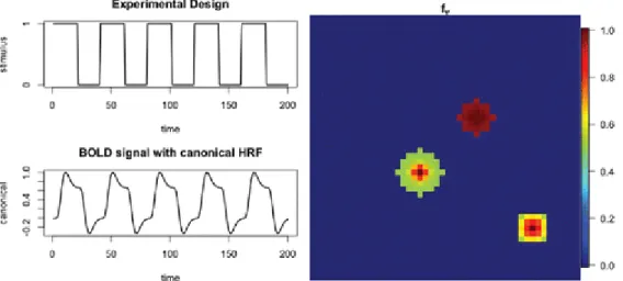
The top left plot in

Figure 1

shows the experimental block design, with st = 1 if the stimulus is on and st = 0

otherwise. It consists of five epochs of 20 sec on and 20 sec off with an observation interval of 1. The resulting BOLD signal zt is shown in the bottom left plot. The right plot displays the active regions with the

corresponding fv values. The three active regions are centered at the coordinates (20, 20), (30, 30), and (40, 10),

with radius arguments 3, 2, 1, and fading arguments 0.5, 0.01, and 0.3, respectively, for each region. The bottom-right region is a square and the other two are circles.

Figure 1.

Left: Block experimental design (top); expected BOLD signal obtained from convolving the stimulus indicator signal with the canonical hemodynamic function (bottom). Right: Activation regions and fv values for

active voxels.

Four different SNRs, 0.5, 1, 5, and 10, and three different CNRs, 0.5, 1, and 1.5, were considered, resulting in 12 different SNR-CNR data types. These are numbered as shown in Table 1. We generated 20 simulated datasets for each SNR-CNR data type and computed classification performance measures (sensitivity, specificity, precision, and accuracy) to examine how well our algorithm and other methods perform in the different scenarios.

Table 1. Twelve data types and their corresponding SNR and CNR.

SNR 0.5 1 5 10

CNR 0.5 1 1.5 0.5 1 1.5 0.5 1 1.5 0.5 1 1.5

Data type 1 2 3 4 5 6 7 8 9 10 11 12

Four methods are compared in this simulation study, the proposed Bayesian complex-valued model using the C-EMVS algorithm for posterior computations (referred to as CV in the results below), the Bayesian magnitude-only model with the EMVS algorithm (MO), and the lasso (LA) and adaptive lasso (ALA), both for magnitude-only data.

The Bayesian complex-valued model used here has the form

𝑦𝑦

𝑡𝑡

𝑣𝑣

=

𝛾𝛾

1

∗

+

𝛾𝛾

2

∗

,

𝑣𝑣

𝑥𝑥

𝑡𝑡

+

𝜂𝜂

𝑡𝑡

𝑣𝑣

,

𝜂𝜂

𝑡𝑡

𝑣𝑣

∼

CN

1

(0,2

𝜎𝜎

2

,0),

with γ*1a baseline parameter and γ*, v2 the complex-valued activation parameters for each voxel and xt = zt. For

the baseline parameter, we use a prior of the form π(γ*1)∝1. For the activation parameters and the remaining

model parameters, we used the following priors:

𝛾𝛾

2

∗

,

𝑣𝑣

∣ 𝜓𝜓

𝑣𝑣

∼

(1

−𝜓𝜓

𝑣𝑣

)CN

1

(0,2

𝑣𝑣

0

𝜎𝜎

2

,0) +

𝜓𝜓

𝑣𝑣

CN

1

(0,2

𝑣𝑣

1

𝜎𝜎

2

,0),

𝜎𝜎

2

∼

IG(1/2,1/2),

𝜓𝜓

𝑣𝑣

∣ 𝜃𝜃 ∼

Bernoulli(

𝜃𝜃

),

𝜃𝜃 ∼

Beta(1,1).

TheFigure 2_{baseline parameter was integrated out before proceeding with the C-EMVS or MCMC algorithms for} posterior inference and detection of active sites, so we used the algorithms outlined in Section

2

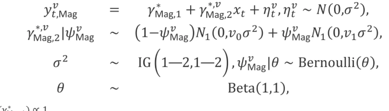
and detailed in the online Appendices.

We also consider a Bayesian model for the magnitude-only data. The magnitude-only time courses are obtained as 𝑦𝑦_𝑡𝑡𝑣𝑣_{,Mag=�(𝑦𝑦}

𝑡𝑡𝑣𝑣,𝑅𝑅𝑅𝑅)2+ (𝑦𝑦𝑡𝑡𝑣𝑣,𝐼𝐼𝐼𝐼)2. The MO model used to analyze these data is essentially the same as the CV

model used for the complex-valued data, except that the linear model is now real-valued and the priors on the regression coefficients are real-valued Gaussian spike-and-slab priors. This is

𝑦𝑦

_𝑡𝑡𝑣𝑣_,Mag

=

𝛾𝛾

Mag∗ ,1

+

𝛾𝛾

Mag∗,𝑣𝑣 ,2

𝑥𝑥

𝑡𝑡

+

𝜂𝜂

𝑡𝑡𝑣𝑣

,

𝜂𝜂

𝑡𝑡𝑣𝑣

∼ 𝑁𝑁

(0,

𝜎𝜎

2

),

𝛾𝛾

Mag∗,𝑣𝑣,2

|

𝜓𝜓Mag

𝑣𝑣

∼ �

1

−𝜓𝜓Mag

𝑣𝑣

�𝑁𝑁

1

(0,

𝑣𝑣

0

𝜎𝜎

2

) +

𝜓𝜓Mag

𝑣𝑣

𝑁𝑁

1

(0,

𝑣𝑣

1

𝜎𝜎

2

),

𝜎𝜎

2

∼

IG

�

1 2,1 2

�

,

𝜓𝜓Mag

𝑣𝑣

|

𝜃𝜃 ∼

Bernoulli(

𝜃𝜃

),

𝜃𝜃

∼

Beta(1,1),

and 𝜋𝜋(𝛾𝛾Mag∗ ,1)∝1..

The tuning parameters in the Bayesian CV and MO models above, v0 and v1, are chosen as suggested in Rockova

and George (2014) and Wang et al. (2015). More specifically, we fix v1, taking v1 = 1 and choose the optimal v0 in

each case, denoted as 𝑣𝑣0CV and 𝑣𝑣0MO,, for the CV and MO models, respectively, by maximizing the marginal

posterior 𝜋𝜋₀(𝛙𝛙 ∣y) that evaluates 𝛙𝛙 according to the submodel that contains only those variables for which ψv j =

1. This marginal can be derived in closed form up to a normalizing constant. From our experience with the real and simulated datasets analyzed here, the optimal v0 takes values around 1⁄�100𝑇𝑇𝑝𝑝 and usually lies in the

interval (1/�1000𝑇𝑇𝑝𝑝, 1/�10𝑇𝑇𝑝𝑝), where p is the number of tasks. In this simulation, we only have one task so p = 1.

Finally, we also applied the lasso (LA) and adaptive lasso (ALA) methods (Tibshirani 1996; Zou 2006) to the magnitude-only data. Both LA and ALA use a regularization parameter and ALA uses additional weights to allow for different penalizations in the regression coefficients (the 𝛾𝛾Mag∗,𝑣𝑣,2 parameters in our case). The regularization

parameter was chosen using a five-fold cross-validation approach and the weights in the ALA were set

to 1 |⁄ 𝛾𝛾�Mag∗,𝑣𝑣,2|,, where 𝛾𝛾�Mag∗,𝑣𝑣,2 is the ordinary least-square estimator of 𝛾𝛾Mag∗,𝑣𝑣,2. LA and ALA were implemented using

the R package glmnet (Friedman, Hastie, and Tibshirani 2010).

The resulting average performance measures over the 20 simulated datasets for the four different methods are summarized in

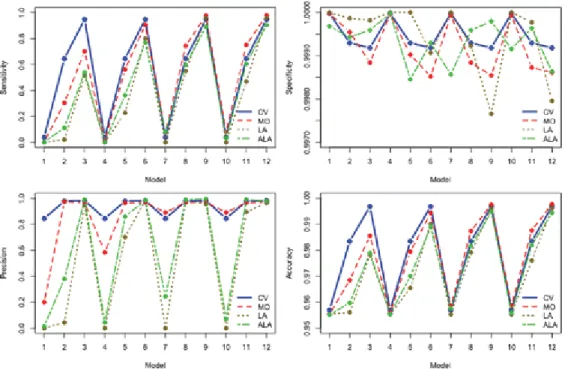
Figure 2

. Note that this simulation contains 2201 nonactive voxels out of a total 2304 voxels, so any model can achieve 95.53% accuracy by simply classifying all voxels as nonactive. Hence, the accuracy subfigure is plotted from 0.95 to 1 for clear comparison. Similarly, the specificity is plotted from 0.997 to 1.

Figure 2.

Sensitivity (top-left), specificity (top-right), precision (bottom-left), and accuracy (bottom-right) for four models: Complex-valued EM (CV; blue, solid), magnitude-only EM (MO; red, dash), Lasso (LA; brown, dotted), and adaptive Lasso (ALA; green, dash-dotted).

First, we seeFigure 3_{that both Bayesian variable selection approaches, the one for the CV-fMRI and the one for} magnitude-only data (MO), dominate the traditional lasso (LA) and adaptive lasso (ALA) for magnitude-only data in terms of sensitivity (power), precision, and accuracy. The Bayesian approaches are able to eliminate most of the false positives by borrowing strength across voxels via the common probability of activation parameter θ. The Bayesian CV and MO methods are comparable to lasso and adaptive lasso in terms of specificity, while the first provide a more complete inferential analysis. The main advantage of the Bayesian CV model with respect to the Bayesian MO model is that the CV model significantly detects more true positives than the MO when the SNR is small, which leads to higher sensitivity, precision, and accuracy. When the SNR is fairly large, using the

information provided only by the magnitude leads to good activation results in these simulated scenarios. In fact, the MO model even has a slightly larger sensitivity than the CV model when the SNR is 5 or 10. On the other hand, the CV model leads to higher specificity and precision than the MO model even when the SNR is 5 or 10.

Moreover, the performance of the CV model is very consistent across different SNRs. Hence, when the CV-fMRI data are recorded under small SNRs or when researchers are uncertain about the magnitude of the SNR in their data, the CV model stands out as the best option among the models considered here. Given that improved MRI technology allows for improved spatial resolution and therefore reduces SNR, we would expect that complex-valued models will become an essential tool for detecting active sites in CV-fMRI data.

Figure 3 shows the true activation and strength maps for one of the 20 simulated datasets with SNR = 0.5 and CNR = 1 along with the estimated activation and strength maps (only for sites labeled as active) obtained from the C-EMVS (CV), the magnitude-only C-EMVS (MO), and adaptive lasso (ALA). The strength maps for lasso are not shown, as lasso detected no active sites. Both activation maps for the complex-valued and magnitude-only EMVS display activation levels that result from setting v1 = 1 and choosing the optimal values of v0 for each method as discussed

above. For this dataset and with our prior distribution settings, we found that the optimal values were 𝑣𝑣₀CV ₌

0.0071 and 𝑣𝑣₀MO_{= 0.0056. The C-EMVS approach clearly outperforms all the other approaches: it has higher}

power for detecting active voxels while simultaneously controlling for false positives, and also leads to more accurate estimation of the activation strength (note that MO and ALA clearly underestimate the strength). In relation to this point, we computed the mean squared errors (MSEs) for this simulated dataset under the C-EMVS, MO, and ALA approaches for voxels that are labeled as active for at least one of the three methods and found that the MSEs values were, respectively, 0.0080, 0.0084, and 0.1162. The complex-valued model also leads to more accurate inference for σ. Magnitude-only models underestimate σ when the SNR is small as a consequence of the

fact that the MO error distribution is truly Ricean at low SNRs. This can lead to an increase of false positives when detecting activation (in fact, we can see that the specificity values obtained with the complex-valued model are generally higher than those obtained with magnitude-only model as shown in Figure 2). For example, for a dataset generated under a true value of σ = 0.5, when SNR = 0.5, we found 𝜎𝜎�CV= 0.497, while 𝜎𝜎�MO= 0.346. To obtain

better estimates of σ with MO models, we need to considerably increase the SNR. For instance, for a simulated dataset with SNR = 10, we obtained 𝜎𝜎�MO= 0.495 which is closer to the true value 0.5. These results are

consistent with the findings of Rowe (2005b).

Figure 3. Activation and strength maps for a simulated dataset with SNR = 0.5 and CNR = 1. (a) Activation maps showing the true active sites, and the activation results obtained from C-EMVS, MO-EMVS, Lasso, and Adaptive Lasso. Activated sites are colored in red. (b) Strength maps: true strength and estimated strengths from C-EMVS, MO-EMVS, Lasso, and adaptive Lasso.

Finally, we also implemented the MCMC sampling approach outlined in Section

2

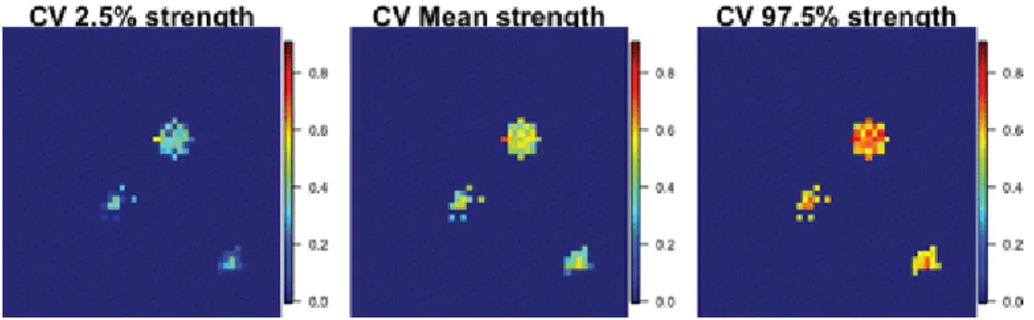
and detailed in the online Appendices to achieve full posterior inference for the complex-valued models. We obtained similar results to those from the C-EMVS algorithm in terms of the number of active sites and the strength of those sites, but we highlight that, in addition, the MCMC approach allows us to compute uncertainty measures related to activation strength and any other functions of the model parameters. For instance,

Figure 4

shows posterior mean strength maps and 95% posterior credibility strength maps for a single dataset obtained from the complex-valued model. As seen in this figure, the posterior mean estimates for the strength are similar to those obtained via the C-EMVS algorithm but the MCMC-based posterior credibility maps provide additional information about the strength maps. We see that, in general, there is less uncertainty about activation strength for voxels located in region centered at (30,30) than for voxels located in the region centered at (40,10). This makes sense given the true strength maps used to generate the simulated data (see

Figure 3

). In cases where this Gibbs sampling scheme is not computationally feasible (e.g., when several large-dimensional images for multiple subjects need to be analyzed), one could consider a hybrid approach that, say, uses the C-EMVS method to determine which sites are active and then uses the Gibbs sampling scheme only on regions of the brain that present active sites to obtain posterior uncertainty measures on strength maps and/or activation maps for those regions only. Alternative methods based on obtaining approximate inference via variational Bayes could also be considered (see, e.g., Yu et al., 2016).

Figure 4.

Strength maps for a simulated dataset with SNR = 0.5 and CNR = 1 obtained from a complex-valued model via MCMC. Left: 2.5% quantile map; Middle: Posterior mean map; Right: 97.5% quantile map.

3.1.1. Additional Structure: Temporal Correlation

We also analyzed synthetic CV-fMRI data simulated under (

11

) but with errors following an autoregressive

structure of order one, that is, ηvt, Re = ϕηt− 1,Rev+ ζvt, Re, with ζvt, Re independent Gaussian for all t, ζvt, Re∼N(0, σ2), and

ηvt, Im = ϕηt− 1,Imv+ ζvt, Im, with ζvt, Im also independent Gaussian for all t, ζvt, Im∼N(0, σ2) and ϕ∈ [0, 1) the AR

coefficient. We considered values of ϕ ranging from 0.1 to 0.9, and the same 12 SNR-CNR scenarios described in the previous simulation, with σ2 _{= 0.25. We analyzed these data using two versions of the model yvt= γ1* +}

γ*, v_{2xt+ ηvt: one version with ηvtiid complex normal, and another version with ηvt following a complex-valued}

AR(1) structure in ηvt= ηt, Rev + iηvt, Im as described above.

Figure 5

displays the sensitivity, specificity, precision,

and accuracy for the two versions of the CV model (independent and autoregressive errors) and two types of data (AR errors with ϕ = 0.5 and ϕ = 0.9). Overall we find that the larger the value of ϕ the harder it is to detect active sites, particularly for small SNR and CNR. This makes sense, as AR(1) errors with ϕ close to 1 may add a temporal structure that locally resembles a linear trend and can easily hide/mask the temporal behavior that characterizes active sites due to increased variability in the observed time series. We also see that while the CV model with independent errors has higher sensitivity, it also leads to a larger number of false positives (we only have about 77% specificity for the model with independent errors while we obtain 100% specificity for the model with AR errors when ϕ = 0.9). Therefore, the CV model with AR errors is overall a better option in terms of specificity, precision, and accuracy, particularly when ϕ is large.

Figure 5.

Sensitivity, specificity, precision, and accuracy plots for synthetic AR(1) CV-fMRI data with AR coefficients 0.5 (top plots) and 0.9 (bottom plots). The plots are based on results obtained from analyzing 20 datasets using models that assumed independent errors (dotted lines) and AR(1) errors (solid lines).

3.1.2. Additional Structure: HRF Effect and Prior Sensitivity Analyses

We also studied the effects of the HRF choice and the prior distributions. Regarding the HRFs, we

analyzed the simulated and human data presented in Sections

3

and 4 with three different classes of HRF

functions, namely, canonical, gamma, and boxcar with different choices for the parameters that define

each particular class. For a given HRF, we can select the optimal

v

0

and then choose the HRF and

corresponding

v

0

that leads to the smallest MSE (mean squared error) for a particular dataset. Overall we

found that the MSEs for the optimal HRFs within each class were comparable. Furthermore, the results in

terms of the number and locations of the sites labeled as active were also similar across the optimal HRFs

within each class.

We studied the sensitivity of our posterior results with respect to the prior distributions. In particular, as

mentioned above, we generally assume θ

∼

Beta(1, 1). In cases where a sparser structure is desired a

priori, that is, when it makes sense biologically to assume that the number of active sites is just a very

small percentage of the total number of sites, priors of the form θ

∼

Beta(1,

b

) with

b

large can be used.

In this simulation study, we found that the activation results were essentially the same for any prior

with

b

⩽

1000. Priors with values of

b

> 1000 lead to sparser results (i.e., less active sites) in the simulated

data. For the human data presented in Section

4

, we found that we are able to detect similar numbers

and locations of active sites for priors with values of

b

∈

[1, 100, 000]. Note that choosing

b

= 1000 leads

to a fairly informative prior, with about 0.09% of active sites expected a priori and rarely above 0.4% of

active sites expected a priori.

Finally, we assessed the effect of using noncircular complex-normal priors on 𝛄𝛄𝑣𝑣_{,, that is, priors of the form 𝛄𝛄}𝑣𝑣 _∣

𝛙𝛙𝑣𝑣 _∼CN

𝑝𝑝(𝟎𝟎,𝜎𝜎𝑣𝑣2𝛀𝛀𝑣𝑣,𝜎𝜎𝑣𝑣2𝚲𝚲𝑣𝑣), with 𝚲𝚲𝑣𝑣 ≠ 𝟎𝟎,, so that there is a nonzero correlation between the real and imaginary

components of 𝛄𝛄𝑣𝑣_{.. As expected, allowing for a correlation structure between the real and imaginary components}

of 𝛄𝛄𝑣𝑣_{. leads to improved results when such underlying structure is present in the data, that is, having a more}

flexible prior that accounts for this correlation leads to higher power for detecting activation and reduces the number of false positives. On the other hand, such priors also lead to models that are more computationally costly and may potentially lead to biases in the posterior results. Therefore, we recommend the use of noncircular priors only when there is a strong indication that there is a significant correlation between the real and complex components of 𝛄𝛄𝑣𝑣_{., and that such correlation structure is similar for active and nonactive voxels. Alternative priors}

noncircular priors in the analysis of a simulated dataset with high correlation among the real and imaginary components for both types of voxels, active and nonactive. The data were simulated following:

𝑦𝑦

𝑡𝑡

𝑣𝑣

,

𝑅𝑅𝑅𝑅

=

�𝛽𝛽

₀

+

𝛽𝛽

1

𝑣𝑣

,

𝑅𝑅𝑅𝑅

𝑧𝑧

𝑡𝑡

�𝑐𝑐𝑐𝑐𝑐𝑐

(

𝛼𝛼

₀

) +

𝜂𝜂

𝑡𝑡

𝑣𝑣

,

𝑅𝑅𝑅𝑅

,

𝜂𝜂

𝑡𝑡

𝑣𝑣

,

𝑅𝑅𝑅𝑅

∼ 𝑁𝑁

(0,

𝜎𝜎

2

),

𝑦𝑦

𝑡𝑡

𝑣𝑣

,

𝐼𝐼𝐼𝐼

=

�𝛽𝛽

0

+

𝛽𝛽

1

𝑣𝑣

,

𝐼𝐼𝐼𝐼

𝑧𝑧

𝑡𝑡

�𝑐𝑐𝑖𝑖𝑠𝑠

(

𝛼𝛼

0

) +

𝜂𝜂

𝑡𝑡

𝑣𝑣

,

𝐼𝐼𝐼𝐼

,

𝜂𝜂

𝑣𝑣

𝑡𝑡

,

𝐼𝐼𝐼𝐼

∼ 𝑁𝑁

(0,

𝜎𝜎

2

),

with α0= π/4, σ2= 0.1, SNR = 0.4, β0 = 0.8, and the same zt used in the previous simulation study. In addition, the

parameters βv_{1, Reand β}v_{1, Im were obtained from complex-normal distributions as follows. For active voxels, we}

sampled βv_{1, Re + iβ1, Imv from a complex noncircular normal with mean 0.7 and covariance and relation values that}

lead to a correlation of 0.9 between βv_{1, Reand β}v_{1, Im. For nonactive voxels, we sampled β}v_{1, Re + iβ1, Imv from a}

complex noncircular normal with mean 0 and covariance and relation values that lead to a correlation of 0.9 between βv_{1, Reand β}v_{1, Im. Note that ηvt, Reand ηvt, Im are assumed independent for all the voxels and also across}

time. The location of the active voxels was determined using the same activation map used in the previous simulation and displayed in the left plot of

Figure 3(a)

.

Figure 6

shows the results obtained from a model that uses a noncircular prior on

γv

that captures the induced correlation structure in these coefficients (left plot) and also shows the results obtained using a circular prior that assumes no correlation structure. Clearly, the model with a noncircular prior leads to much better results as it adequately identifies the active regions and leads to a much smaller number of false positives than those

obtained under the model with the circular prior. The model with the noncircular prior also leads to better results in terms of estimation of activation strength and reduced MSE.

Figure 6.

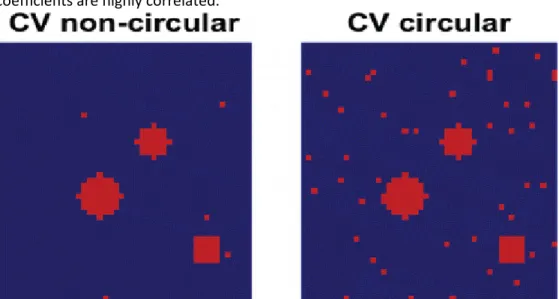
Left: Activation results obtained from a model with a noncircular prior. Right: Activation results

obtained with a circular prior. The data were simulated so that the real and complex components of the activation coefficients are highly correlated.

3.2. Simulation Study II: Physically Realistic Simulated Data

A more realistic simulated dataset was

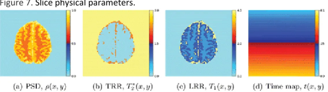
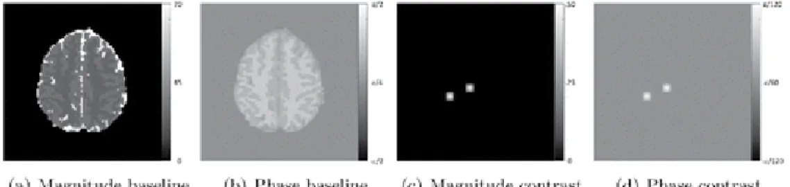
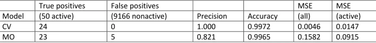
Figure 7, Figure 8

generated using a discrete version of the

magnetic resonance (MR) signal equation after steady-state magnetization (Karaman, Bruce,

and Rowe

2015

). This equation is given by

𝑐𝑐

(

𝑘𝑘

𝑥𝑥

,

𝑘𝑘

𝑦𝑦

∣ 𝑡𝑡

) =

∫

−∞

∞

∫

−∞

∞

𝜌𝜌

(

𝑥𝑥

,

𝑦𝑦

)

𝑅𝑅

−𝑡𝑡

/

𝑇𝑇

2∗

(

𝑥𝑥

,

𝑦𝑦

)

×

�

1

−𝑅𝑅

−𝑇𝑇𝑅𝑅

/

𝑇𝑇

1

(

𝑥𝑥

,

𝑦𝑦

)

�𝑅𝑅

𝑖𝑖𝛤𝛤

𝐻𝐻

𝛥𝛥𝛥𝛥

(

𝑥𝑥

,

𝑦𝑦

)

𝑡𝑡

𝑅𝑅

−𝑖𝑖2𝜋𝜋

(

𝑘𝑘

𝑥𝑥

𝑥𝑥+𝑘𝑘

𝑦𝑦

𝑦𝑦

)

𝑑𝑑𝑥𝑥𝑑𝑑𝑦𝑦

,

(13)

where

s

(

k

x

,

k

y

|

t

) is the

k

-space location at intra slice time

t

, ρ(

x

,

y

) is the proton spin density

(PSD),

T

*

2

(

x

,

y

) is the transverse relaxation rate (TRR),

T

1

(

x

,

y

) is the longitudinal relaxation rate

(LRR), Δ

B

(

x

,

y

) is the magnetic field inhomogeneity (MFI), and Γ

H

is the proton gyromagnetic ratio

(Haacke et al.

1999

Haacke, E., Brown, R., Thompson, M., and Venkatesan, R. (1999),

Magnetic

Resonance Imaging: Principles and Sequence Design

, New York: Wiley.

[Google Scholar]

). The

k

-space points in (

13

) are defined by the temporal integral of the magnetic field gradients

G

x

( · )

and

G

y

( · ):

𝑘𝑘

𝑥𝑥

=

2

𝛤𝛤

𝐻𝐻

𝜋𝜋 � 𝐺𝐺

𝑥𝑥

(

𝑡𝑡

′

)

𝑑𝑑𝑡𝑡

′

,

and

𝑘𝑘

𝑦𝑦

𝑡𝑡

0

=

𝛤𝛤

𝐻𝐻

2

𝜋𝜋 � 𝐺𝐺

𝑦𝑦

(

𝑡𝑡

′

)

𝑑𝑑𝑡𝑡

′